Penalized regression approaches to testing for quantitative
trait-rare variant association
Sunkyung Kim1
, Wei Pan1
* and Xiaotong Shen2
1Division of Biostatistics, School of Public Health, University of Minnesota, Minneapolis, MN, USA 2School of Statistics, University of Minnesota, Minneapolis, MN, USA
Edited by:
Bingshan Li, Vanderbilt University, USA
Reviewed by:
Minghua Deng, Peking University, China
Rui Feng, University of Pennsylvania, USA
*Correspondence:
Wei Pan, Division of Biostatistics, School of Public Health, University of Minnesota, Mayo Bldg/Delaware St SE, MMC 303, Minneapolis, MN 55455–0392, USA
e-mail: [email protected]
In statistical data analysis, penalized regression is considered an attractive approach for its ability of simultaneous variable selection and parameter estimation. Although penalized regression methods have shown many advantages in variable selection and outcome prediction over other approaches for high-dimensional data, there is a relative paucity of the literature on their applications to hypothesis testing, e.g., in genetic association analysis. In this study, we apply several new penalized regression methods with a novel penalty, called TruncatedL1-penalty (TLP) (Shen et al., 2012), for either variable selection, or both variable selection and parameter grouping, in a data-adaptive way to test for association between a quantitative trait and a group of rare variants. The performance of the new methods are compared with some existing tests, including some recently proposed global tests and penalized regression-based methods, via simulations and an application to the real sequence data of the Genetic Analysis Workshop 17 (GAW17). Although our proposed penalized methods can improve over some existing penalized methods, often they do not outperform some existing global association tests. Some possible problems with utilizing penalized regression methods in genetic hypothesis testing are discussed. Given the capability of penalized regression in selecting causal variants and its sometimes promising performance, further studies are warranted. Keywords: GWAS, SSU test, SSUw test, Sum test, TLP
1. INTRODUCTION
Genome-wide association studies (GWAS) have uncovered many common variants (CVs) associated with complex diseases, but the proportion of variance explained by the identified CVs is often low (Maher, 2008). With the recent advance of sequencing technologies, analysis of rare variants (RVs) has become a feasi-ble alternative. Recent studies have demonstrated that some RVs are associated with complex disease. For example,Kotowski et al. (2006) found that multiple RVs in gene PCSK9 are associated with plasma levels of low-density lipoprotein cholesterol.
In this study, we propose applying some new penalized regres-sion methods to test for association between a quantitative trait and multiple RVs. Differing from the usual application of penal-ized regression methods to variable selection or risk prediction for high-dimensional data (Kooperberg et al., 2010; Austin et al., 2013), here we focus on their application to hypothesis testing on a quantitative trait in a relatively low-dimensional setting. In such a setting, one commonly used statistical test is the F-test in linear regression. For example, in simple regression, a traitY is regressed on each of multiple variants sequentially. However, because of the extremely low minor allele frequency (MAF) of a RV, a test to detect the association between a trait and a single RV might be low powered. Also, this approach may be too conservative due to a stringent control for mul-tiple testing, e.g., by the Bonferroni correction to control the family-wise error rate. In addition, ultimately, complex diseases
are expected to be affected by a combination of multiple genetic variants. Thus an analysis in which a group of variants are tested simultaneously for their joint effects on the trait may be more powerful. In multiple regression, to assess any asso-ciation between a trait and k RVs, all k RVs are added to a regression model. However, ask increases, the statistical power might decrease due to the cost of large degrees of freedom (DF), k. To avoid the large DF and to aggregate information across multiple RVs, one common strategy is to pool or collapse mul-tiple RVs in a region or gene (Li and Leal, 2008; Madsen and Browning, 2009). One such attempt is the Sum test (Pan, 2009), which was developed to utilize joint effects of multiple variants while reducing the DF. With only 1 DF, the Sum test enhances power under some scenarios (Chapman and Whittaker, 2008; Pan, 2009). However, it is noted that the performance of the Sum test depends on the directions of the variants’ associations with a trait. Thus, in an extreme case where a half of the vari-ants are positively associated with the trait and the other half are negatively associated with similar effect sizes, the positive and negative effects may cancel out, leading to the poor perfor-mance of the Sum test and other burden tests (Han and Pan, 2010; Li et al., 2010). In addition, in the Sum test or other pooling-based burden tests, combining or collapsing all variants into just one group ignores the variants’ possibly varying effect sizes, and thus may not work well in those situations. In par-ticular, the Sum test and many burden tests perform poorly if
many null (i.e., non-associated) RVs are present (Basu and Pan, 2011). Consequently, the Sum test and other pooled association tests might be low powered.
On the other hand, to deal with high-dimensional genetic and genomic data, penalized regression methods have received much attention, especially those based on the Lasso penalty (Tibshirani, 1996; Kooperberg et al., 2010). Penalized regression has been considered attractive for its potential of simultaneous variable selection and parameter estimation. In particular, several authors have studied the performance of penalized regression in genetic association analysis (Guo and Lin, 2009; Tzeng and Bondell, 2010; Zhou et al., 2011). However, the penalties used therein are typi-cally based on the Lasso, which is known to give biased parameter estimates and possibly inconsistent variable selection. In contrast, one of the very recently developed state-of-the-art penalties, the truncated L1-penalty (TLP) (Shen et al., 2012), overcomes the
above shortcomings of Lasso. The TLP approximates theL0-loss
and reduces the bias of a parameter estimate from the popular Lasso orL1-penalty. To investigate whether an application of TLP
would boost statistical power in genetic association testing, in this study we apply the TLP for variable selection, denoted TLP-S, and for both variable selection and parameter grouping (Zhu et al., 2013), denoted TLP-SG, in a data-adaptive way, to select and group variants to reduce the DF as in the Sum test, while reducing the downward bias of the parameter estimates based on an L1-type penalty. We compare the TLP-S and TLP-SG to
the Lasso and graph-fused Lasso (gflasso) (Kim and Xing, 2009). The gflasso also pursues parameter grouping with anL1-penalty.
Specifically, the gflasso shrinks two variants’ effect sizes toward each other by penalizing their difference|βj−r(j,j)βj|, where eitherr(j,j)=1 (called gflassor=1) orr(j,j) is the sign of the
correlation between the two variantsjandj(called flassor=cor). There are two main differences between our proposed TLP-SG and gflasso. First, TLP-SG shrinks the absolute values of the two parameters toward each other by penalizing|βj| − |βj|. In this way, it desirably allows two variants to have similar effect sizes but opposite association directions. However, such a penalty is non-convex and thus computationally more challenging. Second, by the use of TLP-based grouping (see details later), TLP-SG shrinks|βj| and|βj|toward each other only if their difference is relatively small (as compared to a tuning parameter to be decided), thus, for example, avoiding severely biasing the estimate of the effect size of an associated variant toward 0 by shrink-ing it toward the null effect of a null variant. We note that, although penalized regression methods have been widely used and studied, their applications to the current context with RVs are much more limited; in particular, we are not aware of any applications of TLP-S, TLP-SG and gflasso to association testing of RVs.
This paper is organized in four sections. Section 2 provides a brief review of some existing association tests to be compared, and then introduces our proposed TLP-based tests. In section 3, we compare the performance of the methods with simulated data and with an application to the Genetic Analysis Workshop 17 (GAW17) sequence data (Almasy et al., 2011). Finally, the Discussion section summarizes the results, and suggests some potential problems for future study.
2. METHODS
2.1. SOME EXISTING ASSOCIATION TESTS
We briefly review some existing global tests based on the ordinary least squares (OLS) estimates. Givennindependent observations (Yi,Xi),i=1, . . . ,n,withYi as a quantitative trait and a vec-torXi=(Xi1, . . . ,Xik) as genotypes ofkvariants for subjecti, we
would like to test for any possible association between the trait and genotypes. We use the dosage coding forXij:Xij=0, 1, or 2, representing the count number of one of the two alleles present in variantjof subjecti. A multi-locus association analysis is based on fitting a linear model,
Yi=β0+
k j=1
Xijβj+i (1)
where the errors i are assumed to be independently drawn from N(0, σ2), a Normal distribution with mean 0 and vari-anceσ2. A global test of any possible association between the trait andk variants can be formulated as testing on the mul-tiple parameters βjs for j=1, . . . ,k with null hypothesis H0:
β=(β1, . . . , βk)=0 by anF-test, which is based on the OLS
estimates that minimize the residual sum of squares. A potential problem with the test is the power loss due to the large variance ofβjˆ since the MAFs of RVs are small.
We also apply other four association tests: the Score, the sum of squared score (SSU), its weighted version SSUw (Pan, 2009), and the univariate minP (UminP) tests. The Score test is popular in general statistics while the UminP test is most widely used for CVs in GWAS; on the other hand,Basu and Pan(2011) showed that the SSU and SSUw tests were powerful in RV association test-ing for case-control studies. Here, as a secondary contribution, we extend the SSU and SSUw tests to the case with a quantita-tive trait. All the four tests are based on the score vectorUand its covariance matrixVunderH0:
U = n i=1 (Yi− ¯Y)Xi, V =Cov(U)= ˆσo2 n i=1 (Xi− ¯X)(Xi− ¯X)T, whereY¯ =ni=1Yi/n,X¯ = n i=1Xi/n, andσˆo2= n i=1(Yi− ¯
Y)2/(n−1) is the estimate ofσ2underH0. The corresponding
four test statistics are
TScore=UTV−1U, TSSU =UTU,
TSSUw =UTVd−1U with Vd=Diag(V), TUminP =maxk
j=1U 2
j/vj,
whereUjis thejth element ofUandvjis the (j,j)th diagonal ele-ment ofV. UnderH0, asymptoticallyTScorehas aχk2distribution,
each ofTSSU andTSSUw has a mixture of chi-squared distribu-tions (Pan, 2009), and thep-value ofTUminPcan be numerically obtained (Conneely and Boehnke, 2007).
Next, we extend the Sum test (Pan, 2009) and its modi-fied version, a data-adaptive Sum (aSum) test (Han and Pan, 2010), to the case with a quantitative trait. The Sum test was originated to model multiple variants jointly while induc-ing a minimum number of DF: while includinduc-ing all the vari-ants in the linear model, it assumes that the varivari-ants all have the same effect size (and direction), βc, as in the following model: Yi=βc,0+ k j=1 Xijβc+i (2)
Fitting (Equation 2) is equivalent to conducting a simple regres-sion ofYon a new covariate, the sum of the genotypes over the multiple variants. To address the question of whether any associa-tion between the disease and the variants exists, one simply needs to testH0:βc=0, without the need for multiple testing
adjust-ment. The main advantage of the Sum test is that, because it tests on only one parameterβc, there will be no power loss due to the large DF. The common association parameterβc is a weighted average of the individualβM,1, . . . , βM,kin the marginal mod-els Yi=βM,0+XijβM,j+ij for j=1, . . . ,k (Pan, 2009). On the other hand, the main problem of the Sum test is its depen-dence on the signs ofβM,js or on the coding of each variant (i.e., which allele is chosen as the reference category). If the signs are not the same, the test may have a quite smallβcˆ and thus low power. To overcome the limitation of the Sum test,Han and Pan (2010) proposed the aSum test for a case-control study design, which can be equally applied to quantitative traits as the fol-lowing. (1) For each variantj, flip its coding toX.∗j=2−X.jif
ˆ
βM,j<0 and itsp-valuepM,j≤α0in the marginal model;
other-wise use the same codingX∗.j=X.j. (2) Fit the model (Equation 2) with the new coding X∗. To testH0 in the aSum test, we use
a permutation-based log-likelihood ratio test (LRT), which is asymptotically equivalent to the score test. For the choice ofα0,
we use the same value as recommended byHan and Pan(2010), 0.1, to prevent reduced power when a too small or too largeα0is
used.
While theF-test is based on OLS estimates, in next section we apply some penalized regression methods, the Lasso, gflasso and a recently developed TLP for either only variable selection (TLP-S) or both variable selection and parameter grouping (TLP-SG). In short, both the Lasso and TLP-S consider only variable selection, while the gflasso and TLP-SG pursue parameter grouping along with variable selection to improve power by striking a better bal-ance between goodness-of-fit and reduced DF in the joint model (Equation 1).
2.2. PENALIZED REGRESSION BASED TESTS
2.2.1. Parameter estimation from penalized regression
Given a vector of traitsY=(Y1, . . . ,Yn)and a design matrix for
kvariantsX=(X·1, . . . ,X·k), the Lasso estimate ofβis obtained from the penalized least squares function:
ˆ β=argmin β 1 2Y−Xβ 2+λ k j=1 |βj|, (3) where a largeλautomatically yields some components ofβˆas 0, realizing variable selection. While Lasso does effective vari-able selection, its estimates are always biased. To overcome the issue,Shen et al.(2012) proposed a truncated Lasso(L1)-penalty
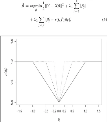
(TLP)Jτ(|x|)=min(|τx|,1), which, asτ→0+, tends to theL0
-loss,I(|x| =0). The degree of approximation by TLP is controlled by a tuning parameter, τ. See Figure 1 for a display over the different values ofτ. Then the TLP-estimateβˆis obtained from
ˆ β=argmin β 1 2Y−Xβ 2+λ 1 k j=1 Jτ(|βj|), (4)
and we denote (Equation 4) as TLP-S. The most interesting fea-ture of the TLP is that only smaller|βj|’s less than a thresholdτare penalized, hence realizing variable selection (if some are shrunken to 0) while avoiding penalizing larger|βj|’s and thus leading to their almost unbiased estimates.
While both the Lasso and TLP-S consider only variable selec-tion, an alternative way to reduce model complexity is grouping pursuit (Shen and Huang, 2010). To investigate the grouping effects on a test’s power, we apply two recent penalized group-ing methods, gflasso and TLP-SG. Theβestimate from gflasso is based on the following objective function:
ˆ β =argmin β 1 2Y−Xβ 2+λ 1 k j=1 |βj| +λ2 j<j |βj−r(j,j)βj|, (5)
FIGURE 1 | TruncatedL1-penalty (TLP) functionJτ(|βj|) withτ=0.2, 0.5, and 1 (as solid, dashed and dotted lines, respectively).
where the first penalty is used for variable selection and the sec-ond is to encourage parameter grouping. r(j,j) is the sign of the correlation between two variantsX·jandX·j, which is used to approximate the target |βj| ≈ |βj|; this method is denoted gflassor=cor. On the other hand, ifr(j,j)=1 is used, the penalty targetsβj≈βj.
The TLP-SG estimate ofβcomes from ˆ β=argmin β 1 2Y−Xβ 2+λ 1 k j=1 Jτ(|βj|) +λ2 j<j Jτ(|βj| − |βj|), (6)
where the first penalty is for variable selection while the sec-ond shrinks the difference of|βj|’s if a difference is within the upper boundτ. The number of the groups of equal parame-ter estimates is a decreasing function of λ2. Thus, the tuning
parameters (λ1, λ2, τ) are selected to balance between the model
complexity and model goodness-of-fit, which presumably may contribute to enhanced power. As a comparison, in the Sum test all parameters (or variants) are forced to belong to the same sin-gle group even if the variants’ associations with the trait are quite different both in effect sizes and directions; the TLP-SG method attempts to conduct a more precise grouping over all variants in a data-adaptive way.
To computeβ in Lasso, gflasso, TLP-S and TLP-SG, we used the Feature Grouping and Selection Over an Undirected Graph (FGSG) package ofYang et al.(2012), which is a C library with interface to MATLAB and is quite fast to run. Its computing effi-ciency allowed us to estimate separate tuning parameters for each permuted dataset to control the type I error as explained in the next section.
2.2.2. Hypothesis testing
To test the null hypothesisH0:β=0 in Equation (1), we
con-duct a permutation-based test, in which thep-value is calculated by comparing a test statisticTapplied to the original dataset to the onesT0(b)applied to theBpermuted datasets forb=1, . . . ,B. We use permutation to control the Type I error since the null distri-bution of a test statistic based on a penalized regression estimate is in general difficult to obtain. The permutation-based testing procedure follows:
Step 1. With the original data {(Yi,Xi)}, we solve a penalized regression problem to obtainβˆin Equation (1).
Step 2. Calculate a test statisticT=T(βˆ).
Step 3. By repeatedly permuting the observedY of the original data, we obtainBsets of permuted data{(Yi(b),Xi)}for b=1, . . . ,B. For each permuted data set,{(Yi(b),Xi)}, we repeat the Steps 1 and 2, obtaining the null statisticsT(0b). Step 4. The finalp-value isBb=1IT<T0(b)/B.
We apply each of several test statistics in Step 2. First, across all penalized methods, we use a 1-dfF-statistic (1-df) to test the asso-ciation betweenYandXβˆ, whereβˆis the penalized estimate ofβ
in Step 1. Specifically, we fit a linear model Yi=α0+
Xiβˆα+i,
and testH0:α=0 . This 1-df test uses variable selection and pos-sibly parameter grouping result from the corresponding penalized method, while allowing testing with only 1 DF. Second, for TLP-SG, we also apply the corresponding SSU and SSUw tests, where the test statisticsTSSU andTSSUw are both based on the selected variables from the corresponding penalized estimates. Specifically,
TSSU =U∗U∗,
TSSUw=U∗(Vd∗)−1U∗ with Vd∗=Diag(V∗), whereU∗is a sub-component vector of the score vectorU corre-sponding to| ˆβj| =0, and| ˆβj|>0.001 is considered as non-zero. Similarly,V∗is the corresponding sub-matrix of the covariance matrixV. Note that the grouping information is not used. 2.2.3. Selection of tuning parameters
To select the suitable tuning parameters, we apply a grid-search with Akaike’s information criterion (AIC) (Akaike, 1974):
AIC= −2 logL+2p,
where logL=−nlog (σˆ2)−n−p−1/2 is the log-likelihood
with the penalized estimate plugged-into model (Equation 1), andσˆ2=ni=1(Yi−β0−Xiβˆ)2/(n−p−1). The effective
number of the parameters,p, in AIC is computed as the number of non-zero| ˆβj|’s for Lasso and TLP-S, as the number of non-zero uniqueβjˆ’s for gflassor=1, and as the number of non-zero unique
| ˆβj|’s for gflassor=cor and TLP-SG, respectively. Forλin Lasso, the one resulting in the smallest AIC out of 50 equally spaced points in [0.001,10] is selected. Similarly, the values of each ofλ1,
λ2andτ in other methods are searched over five equally spaced
grid points of [0.001,1], [0.001,0.5], and [0.001,0.5], respec-tively. For each permuted dataset (Yi(b),Xi) forb=1, . . . ,B, we also estimate its own (λ(1b), λ(2b), τ(b)) to properly control the type I error.
3. RESULTS 3.1. SIMULATIONS
We consider two simulation schemes. In the first scheme, we gen-erate only RVs with a total of 200 replicates andn=400 in each replicate. The permutation size is set asB=100. For each repli-cate, to generatekvariants including six causal ones in linkage disequilibrium (LD), as inWang et al.(2007), two latent vectors from multivariate normal distribution MVN(0,R) are simulated, whereRhas a first order auto regressive (AR1) structure; the asso-ciation between any two elements of the latent vector decreases by ρ= 0.8 times as 1 lag increases. Then, the vector is dichotomized to yield a haplotype with the minor allele frequency (MAF) of each variant randomly chosen between 0.005 and 0.01. The genotype data Xi=(Xi1, . . . ,Xik) for sample iis obtained by
the randomly located six causal variants withσ2=2 in model (Equation 1), where the interceptβ0is set as 0.3 throughout the
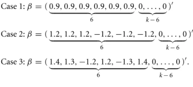
simulations. The considered three cases are: Case 1:β =( 0.9,0.9,0.9,0.9,0.9,0.9 6 ,0 , . . . ,0 k−6 ) Case 2:β =( 1.2,1.2,1.2,−1.2,−1.2,−1.2 6 ,0 , . . . ,0 k−6 ) Case 3:β =( 1.4,1.3,−1.2,1.2,−1.3,1.4 6 ,0 , . . . ,0 k−6 ).
In each case, we vary the number of non-causal RVsk-6 from 0 to 24 so that the total number of RVs,k, ranges from 6 to 30. The Type I error is computed from theYunderH0:β=(0, . . . ,0).
In the second scheme, multiple RVs and two CVs are gener-ated to mimic the GAW17 data we use later. The frequency of one allele for each CV is randomly distributed between 0.2 and 0.7, and CVs may or may not be chosen as a causal variant in each replicate. When a CV is randomly selected as a causal variant, its effect size βj is scaled down to βj/10 in the following cases to prevent its dominating association with the outcome. The considered three cases for mixed RVs and CVs are:
Case 1:β=( 1,1,1,1,1,1 6 ,0 , . . . ,0 k−6 ) Case 2:β=( 1.5,1.5,1.5,−1.5,−1.5,−1.5 6 ,0 , . . . ,0 k−6 ) Case 3:β=( 1.1,1.3,−1.2,1.2,−1.3,1.1 6 ,0 , . . . ,0 k−6 ),
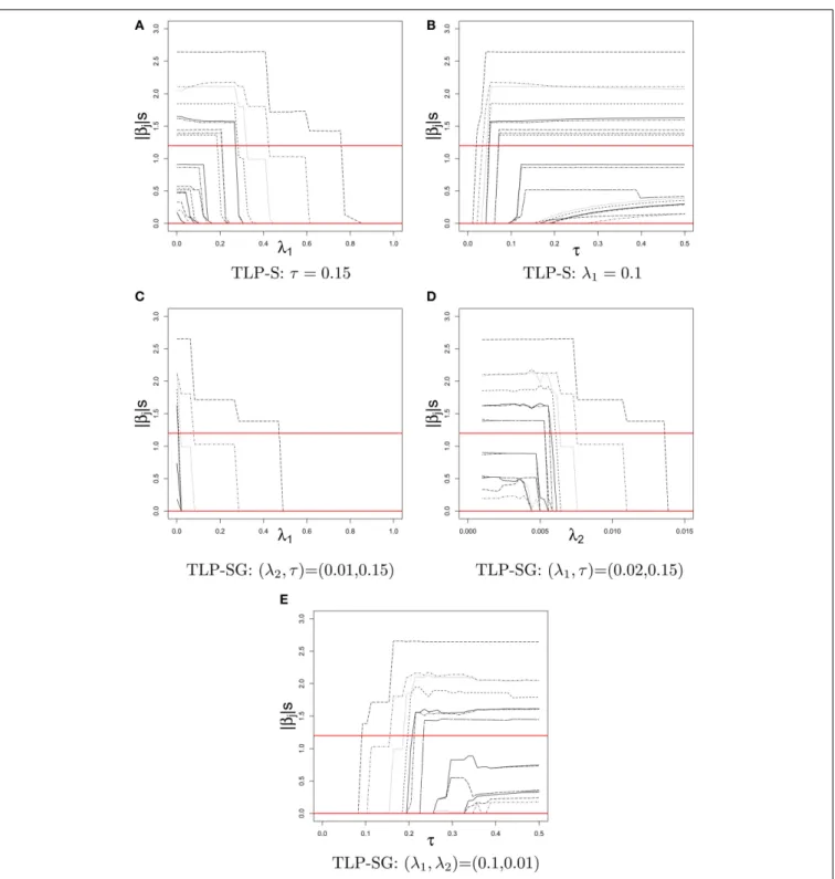
Figure 2displays the TLP-S and TLP-SG solution paths of| ˆβj| over a tuning parameter given other(s), where two horizontal lines at 1.2 and 0 give the true parameter values for Case 2 set-up with only RVs. In contrast to piece-wise linear solution paths of the Lasso estimates, the TLP solution paths are like step functions as expected from anL0-penalty (i.e., best subset selection).
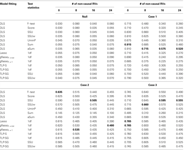
Table 1presents the simulation results for the RVs only set-ups. The Type I error rates seem to be properly controlled under the null for all cases, though there are some slightly inflated num-bers, possibly due to the relatively small number of replicates and/or permutation numbers. Under the alternative hypothe-sis, in Case 1 where the causal associations are all in the same direction, the Sum or aSum test beats other methods. Within the class of penalized regression methods, TLP-SG with the SSU or SSUw test statistics is most powerful; in particular, TLP-SG with the SSUw statistic performs better than theF-test regard-less of the number of non-causal RVs included. There seems to be no gain with grouping in TLP-SG as compared to no group-ing in TLP-S, and the 1df-test of TLP-SG works better than gflassor=corunless the number of non-causal RVs is large at 24. Overall, penalized regression methods do not significantly out-perform the power over the Sum and aSum tests. In Cases 2 and 3, where the causal effect directions are mixed, the Sum
test works poorly as expected, while the aSum test has higher power. Overall, either the SSU or SSUw test is the winner. In par-ticular, the TLP-S- and TLP-SG-based tests do not significantly improve over the SSU and SSUw tests, though they may per-form better than those based on the Lasso and gflasso. Again, a comparison between TLP-S and TLP-SG reveals that param-eter grouping does not seem to contribute much to increased power.
The results of the mixed RVs and CVs set-ups are listed in Table 2. Note that, as discussed in Basu and Pan (2011), with mixed RVs and CVs, the SSU test might not perform well. Overall, the SSUw test is the winner. The penalized methods can perform well in some situations, but they do not always outperform the SSUw test. Among the penalized methods, the proposed TLP-S and TLP-SG are competitive against the Lasso and gflasso.
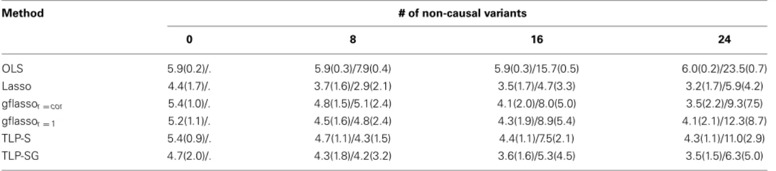
An advantage of penalized methods over global tests is the formers’ ability for variable selection, narrowing down possible causal variants. We note that causal variant selection is an under-studied problem in genetics, which will become more important when we transition from association studies to causal inference. On the other hand, variable selection via penalized methods or any other methods has yet been fully investigated in the current context with largen, smallk, and more importantly with RVs. InTable 3, we investigate their variable selection performance for one simulation set-up; the results for other set-ups are similar and thus omitted. We show the mean numbers of true positives (TP) and false positives (FP), where a| ˆβj|>0.001 is counted as a positive (i.e., non-zero). As expected, the OLS estimates (and the global tests) cannot conduct variable selection with the mean TP and mean FP close to their maximum possible values. Among the penalized methods, a method tends to be either more conser-vative (fewer FP and fewer TP at the same time) or more liberal (higher FP and higher TP). If we look at the ratio of FP over TP, it seems that the Lasso and TLP-SG are best with the highest ratio, especially for a larger number of non-causal RVs.
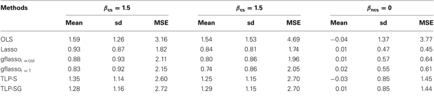
We compare the performance of the parameter estimates in Table 4for one simulation set-up; the results for other set-ups are similar and thus omitted. As expected, the OLS estimates are almost unbiased, but with the largest mean squared errors (MSEs) due to their large variability. The penalized estimates all have smaller MSEs and larger biases than the OLS estimates. Among the penalized methods, the TLP-S and TLP-SG estimates have much smaller biases, but larger variances and thus larger MSEs than those of Lasso and gflasso. In particular, for a causal effect (βc), Lasso and gflasso shrink it more toward 0, while TLP-S and TLP-SG give much less biased estimates.
3.2. MINI-EXOME SEQUENCE DATA
We apply the methods to the mini-exome sequence data from the GAW17 (Almasy et al., 2011). The data set consists of 3205 autosomal genes with 24,487 variants on 697 subjects. The geno-types are obtained from the sequence alignment files provided by the 1000 Genomes Project for the pilot 3 study. The GAW17 data include 200 replicates of three simulated quantitative traits named Q1, Q2, and Q4, where only Q1 and Q2 were influenced by genetic factors. Here we use Q2, which is determined by 72 vari-ants in 13 genes. The true effect sizes of all varivari-ants range from 0.2
FIGURE 2 | Solution paths of| ˆβj|’s in a simulated dataset of Case 2 with
k=22 RVs for TLP-S and TLP-SG over the values of a tuning parameter given other(s).The true values of|βj|’s at 1.2 and 0 are given by two
horizontal lines.(A)TLP-S:τ=0.15.(B)TLP-S:λ1=0.1.(C)TLP-SG: (λ2, τ)=(0.01,0.15).(D)TLP-SG: (λ1, τ)=(0.02,0.15).(E)TLP-SG: (λ1, λ2)= (0.1,0.01).
to 1.2; all variants are positively associated with the trait Q2 but in differential magnitudes.
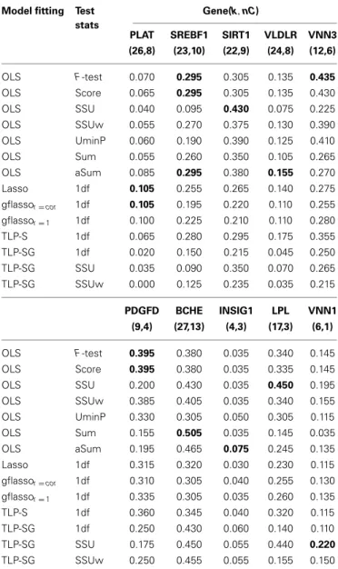
In this study, we test on each of all causal genes (PLAT, SREBF1, SIRT1, VLDLR, VNN3, PDGFD, BCHE, INSIG1, LPL, RARB, VNN1, and VWF) except GCKR, which contains just one SNP. The number of causal variants (nC) in each gene affecting Q2,
and some summary statistics of their MAFs and pairwise correla-tions (COR) are listed inTable 5. Within each gene, most variants are RVs, but a few are CVs with their MAFs larger than 5%. First, we test for any association between Q2 and all variants gene by gene as shown inTable 6, and then test on each gene without its CVs as shown inTable 7.
Table 1 | Empirical Type I error and Power at the nominal levelα=0.05 based on 200 replicates for the RVs only set-ups with six causal RVs and a varying number of non-causal RVs.
Model fitting Test statistics # of non-causal RVs # of non-causal RVs 0 8 16 24 0 8 16 24 Null Case 1 OLS F-test 0.030 0.080 0.040 0.060 0.715 0.480 0.340 0.260 OLS Score 0.030 0.080 0.035 0.055 0.710 0.470 0.320 0.245 OLS SSU 0.030 0.060 0.045 0.045 0.830 0.660 0.510 0.405 OLS SSUw 0.035 0.080 0.055 0.060 0.810 0.625 0.500 0.380 OLS UminP 0.045 0.070 0.050 0.035 0.675 0.445 0.360 0.310 OLS Sum 0.055 0.075 0.040 0.075 0.915 0.685 0.525 0.460 OLS aSum 0.035 0.065 0.035 0.060 0.910 0.715 0.575 0.520 Lasso 1df 0.055 0.075 0.050 0.080 0.710 0.415 0.325 0.270 gflassor=cor 1df 0.035 0.080 0.050 0.090 0.690 0.415 0.240 0.295 gflassor=1 1df 0.035 0.070 0.050 0.075 0.685 0.375 0.225 0.275 TLP-S 1df 0.050 0.085 0.050 0.075 0.720 0.450 0.305 0.255 TLP-SG 1df 0.055 0.085 0.055 0.070 0.700 0.450 0.290 0.250 TLP-SG SSU 0.055 0.080 0.040 0.060 0.700 0.520 0.440 0.390 TLP-SG SSUw 0.040 0.075 0.045 0.070 0.790 0.500 0.365 0.320 Case 2 Case 3 OLS F-test 0.635 0.515 0.440 0.455 0.745 0.640 0.550 0.490 OLS Score 0.625 0.500 0.425 0.395 0.745 0.635 0.525 0.470 OLS SSU 0.590 0.530 0.505 0.445 0.710 0.645 0.595 0.555 OLS SSUw 0.570 0.505 0.475 0.445 0.715 0.660 0.570 0.525 OLS UminP 0.450 0.410 0.400 0.310 0.665 0.595 0.425 0.425 OLS Sum 0.145 0.125 0.145 0.100 0.485 0.310 0.260 0.215 OLS aSum 0.450 0.430 0.355 0.340 0.665 0.590 0.535 0.500 Lasso 1df 0.615 0.465 0.405 0.390 0.765 0.585 0.465 0.435 gflassor=cor 1df 0.620 0.530 0.435 0.480 0.765 0.600 0.480 0.520 gflassor=1 1df 0.615 0.535 0.435 0.425 0.750 0.585 0.475 0.495 TLP-S 1df 0.615 0.505 0.455 0.425 0.760 0.630 0.530 0.475 TLP-SG 1df 0.615 0.485 0.445 0.415 0.755 0.605 0.450 0.450 TLP-SG SSU 0.565 0.470 0.460 0.445 0.705 0.605 0.510 0.525 TLP-SG SSUw 0.585 0.505 0.460 0.415 0.745 0.585 0.485 0.475
Maximum power in bold.
InTable 6, when both RVs and CVs within a gene are included, the identity of the most powerful test differs across the genes: the F-test is the winner for the genes VLDLR, VNN3, PDGFD, and LPL; however, for the genes VLDLR, BCHE, VNN1, and VWF, the SSU or SSUw test is the best. The two gflasso-based tests work quite similarly over all genes. The TLP based tests perform best for the genes SREBF1, RARAB, VNN1, and INSIG1. After remov-ing a few CVs in each gene (Table 7), the SSU test recovers good power for the genes PDGFD, BCHE and LPL. The Sum test is the winner for gene BCHE, while theF-test based on the OLS esti-mates perform best for genes VNN3, SREBF1, and PDGFD. For gene VNN1, the TLP-SG with the SSU statistic has the highest power.
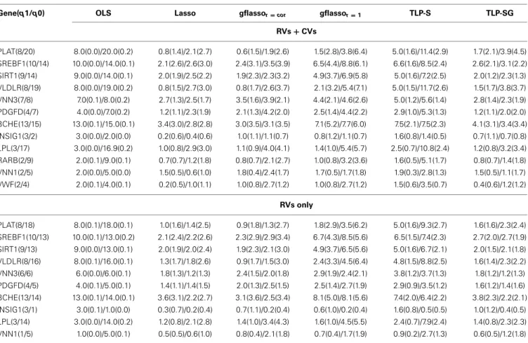
A potential advantage of penalized regression is variable selection, which is missing from existing global tests. Table 8 shows the results of causal variant selection by the penalized methods. Overall, each penalized method could eliminate some
non-associated variants at the cost of omitting some causal ones. In general, in agreement with simulated data, the Lasso and TLP-SG seem to select fewest variants, including both TPs and FP, while TLP-S and gflasso give higher numbers of both TPs and FPs. 4. DISCUSSION
In this study we have conducted hypothesis testing to detect the association between a quantitative trait and multiple RVs based on some new penalized regression methods. In addition to the traditional use of penalized regression for variant selection, we have also considered several state-of-the-art grouping pursuit methods that smooth the effect sizes of the variants, eitherβior |βi|, in a data-adaptive way, which can be considered as a general-ization of the Sum and other genotype pooling/collapsing-based burden tests. In particular, our proposed TLP-SG overcomes sev-eral limitations of the Sum and other burden tests. First, by vari-able selection, the result of TLP-SG is presumably less influenced
Table 2 | Empirical Type I error and Power at the nominal levelα=0.05 based on 200 replicates for the RVs+CVs set-ups with six causal variants and a varying number of non-causal ones.
Model fitting Test statistics
# of non-causal variants # of non-causal variants
0 8 16 24 0 8 16 24 Null Case 1 OLS F-test 0.025 0.045 0.065 0.050 0.760 0.520 0.355 0.385 OLS Score 0.020 0.045 0.065 0.035 0.760 0.515 0.345 0.350 OLS SSU 0.060 0.050 0.090 0.030 0.490 0.210 0.125 0.110 OLS SSUw 0.040 0.035 0.060 0.035 0.845 0.695 0.510 0.510 OLS UminP 0.030 0.055 0.060 0.025 0.715 0.540 0.380 0.410 OLS Sum 0.055 0.060 0.075 0.045 0.695 0.450 0.315 0.315 OLS aSum 0.050 0.060 0.065 0.045 0.665 0.435 0.325 0.340 Lasso 1df 0.030 0.045 0.060 0.045 0.750 0.515 0.360 0.375 gflassor=cor 1df 0.030 0.030 0.070 0.015 0.760 0.450 0.275 0.415 gflassor=1 1df 0.030 0.030 0.070 0.015 0.765 0.455 0.290 0.385 TLP-S 1df 0.035 0.050 0.050 0.030 0.750 0.540 0.360 0.370 TLP-SG 1df 0.035 0.035 0.065 0.045 0.750 0.515 0.335 0.315 TLP-SG SSU 0.075 0.060 0.055 0.065 0.495 0.230 0.140 0.105 TLP-SG SSUw 0.030 0.055 0.055 0.045 0.845 0.675 0.435 0.375 Case 2 Case 3 OLS F-test 0.800 0.765 0.720 0.650 0.655 0.585 0.415 0.375 OLS Score 0.800 0.755 0.710 0.630 0.645 0.580 0.400 0.360 OLS SSU 0.275 0.175 0.155 0.160 0.200 0.140 0.110 0.105 OLS SSUw 0.715 0.705 0.715 0.665 0.640 0.615 0.485 0.415 OLS UminP 0.640 0.615 0.550 0.505 0.530 0.510 0.370 0.345 OLS Sum 0.190 0.120 0.125 0.100 0.195 0.150 0.090 0.110 OLS aSum 0.345 0.275 0.270 0.315 0.290 0.225 0.195 0.210 Lasso 1df 0.805 0.695 0.640 0.585 0.580 0.555 0.415 0.360 gflassor=cor 1df 0.810 0.725 0.625 0.655 0.595 0.570 0.420 0.415 gflassor=1 1df 0.805 0.725 0.620 0.655 0.590 0.570 0.435 0.395 TLP-S 1df 0.790 0.730 0.680 0.615 0.600 0.570 0.395 0.390 TLP-SG 1df 0.795 0.730 0.620 0.600 0.600 0.555 0.400 0.310 TLP-SG SSU 0.310 0.185 0.165 0.210 0.205 0.120 0.125 0.120 TLP-SG SSUw 0.750 0.720 0.650 0.550 0.675 0.560 0.460 0.390
Maximum power in bold.
Table 3 | Mean numbers of TP(sd)/FP(sd) of the methods in Case 2 with both RVs and CVs. Method # of non-causal variants
0 8 16 24 OLS 5.9(0.2)/. 5.9(0.3)/7.9(0.4) 5.9(0.3)/15.7(0.5) 6.0(0.2)/23.5(0.7) Lasso 4.4(1.7)/. 3.7(1.6)/2.9(2.1) 3.5(1.7)/4.7(3.3) 3.2(1.7)/5.9(4.2) gflassor=cor 5.4(1.0)/. 4.8(1.5)/5.1(2.4) 4.1(2.0)/8.0(5.0) 3.5(2.2)/9.3(7.5) gflassor=1 5.2(1.1)/. 4.5(1.6)/4.8(2.4) 4.3(1.9)/8.9(5.4) 4.1(2.1)/12.3(8.7) TLP-S 5.4(0.9)/. 4.7(1.1)/4.3(1.5) 4.4(1.1)/7.5(2.1) 4.3(1.1)/11.0(2.9) TLP-SG 4.7(2.0)/. 4.3(1.8)/4.2(3.2) 3.6(1.6)/5.3(4.5) 3.5(1.5)/6.3(5.0)
When k=6, FP is 0 and denoted as “.” after “/”.
by the presence of many non-associated variants to be tested. Second, rather than pooling all the variants into a single group or two groups, TLP-SG automatically determines the number of groups to be formed based on the given data. Furthermore,
since TLP-SG shrinks the effects sizes|βi|, not βi, toward each other, it is robust to varying association directions of the causal variants. However, based on our studies on both simulated and real sequence data, we found that TLP-SG and other penalized
Table 4 | Means, sd’s and MSEs of some causal (βcs) and non-causal (βncs) variants’ regression coefficient estimates whenk=30 in Case 2
with both RVs and CVs.
Methods βcs=1.5 βcs=1.5 βncs=0
Mean sd MSE Mean sd MSE Mean sd MSE
OLS 1.59 1.26 3.16 1.54 1.53 4.69 −0.04 1.37 3.77 Lasso 0.93 0.87 1.82 0.84 0.81 1.74 0.01 0.47 0.45 gflassor=cor 0.88 0.93 2.11 0.80 0.86 1.96 0.01 0.57 0.64 gflassor=1 0.83 0.92 2.15 0.74 0.86 2.05 0.02 0.55 0.61 TLP-S 1.35 1.14 2.60 1.25 1.15 2.70 −0.03 0.85 1.45 TLP-SG 1.28 1.16 2.72 1.29 1.15 2.70 0.01 0.85 1.44
Table 5 | MAFs (%) and pair-wise correlations (COR) in the values of (min, mean, max) for the 12 genes influencing the quantitative trait Q2 in the GAW17 data.
Gene All Causal Non-causal
PLAT MAF (0.072,2.098,45.12) (0.072,0.206,0.574) (0.072,2.855,45.12) SREBF1 (0.072,0.699,7.747) (0.072,0.222,0.43) (0.072,1.04,7.747) SIRT1 (0.072,0.858,16.71) (0.072,0.12,0.215) (0.072,1.332,16.71) VLDLR (0.072,1.047,9.469) (0.072,0.126,0.287) (0.072,1.435,9.469) VNN3 (0.072,4.429,40.53) (0.072,2.06,9.828) (0.072,6.501,40.53) PDGFD (0.072,4.115,31.56) (0.072,0.287,0.861) (0.072,6.303,31.56) BCHE (0.072,0.625,14.56) (0.072,0.105,0.287) (0.072,1.076,14.56) INSIG1 (0.072,0.775,3.587) (0.072,0.072,0.072) (0.072,1.829,3.587) LPL (0.072,1.854,14.490) (0.072,0.598,1.578) (0.072,2.076,14.490) RARB (0.072,0.352,1.363) (0.072,0.287,0.502) (0.072,0.367,1.363) VNN1 (0.072,2.675,17.070) (0.574,8.824,17.070) (0.072,0.215,0.359) VWF (0.072,0.944,2.080) (0.072,0.323,0.574) (0.359,1.255,2.080) PLAT COR (−0.143,0.002,0.753) (−0.008,−0.003,−0.001) (−0.143,0.007,0.753) SREBF1 (−0.038,0.007,0.635) (−0.009,−0.004,−0.001) (−0.038,0.024,0.635) SIRT1 (−0.044,0.004,0.707) (−0.004,0.007,0.33) (−0.044,0.002,0.499) VLDLR (−0.135,−0.001,0.331) (−0.003,−0.002,−0.001) (−0.135,0.001,0.331) VNN3 (−0.422,−0.002,0.59) (−0.104,−0.01,0.072) (−0.422,−0.001,0.341) PDGFD (−0.156,−0.007,0.276) (−0.007,−0.004,−0.001) (−0.156,−0.007,0.276) BCHE (−0.044,0.001,0.499) (−0.005,0.004,0.499) (−0.044,−0.002,0.075) INSIG1 (−0.010,0.009,0.128) (−0.001,−0.001,−0.001) (0.128,0.128,0.128) LPL (−0.138,−0.002,0.215) (−0.010,−0.006,−0.002) (−0.138,−0.002,0.215) RARB (−0.025,−0.003,0.073) (−0.004,−0.004,−0.004) (−0.025,−0.005,−0.001) VNN1 (−0.046,0.038,0.945) (0.055,0.055,0.055) (−0.005,0.091,0.945) VWF (0.113,0.316,0.564) (0.265,0.265,0.265) (0.127,0.246,0.466)
methods sometimes might be more powerful than some existing global tests, though they do not always outperform the SSU or SSUw test. The discovery of no uniform gain of penalized meth-ods over existing global tests is interesting and even surprising, and can be due to non-optimal implementation of the penal-ized methods in several aspects. First, the selection of the tuning parameters based on the model selection criterion AIC may not be optimal. As an example, in a simulated dataset, when we set the tuning parameters to properly group the variants, the esti-mates were quite close to the true values, but the corresponding AIC was less desirable, leading to choosing other low perform-ing tunperform-ing parameters. Importantly, there is no theory yet to justify the applicability of AIC for the gflasso- and TLP-based
methods; in particular, it is unclear how to count the effective number of parameters in the AIC. Alternatively, one may want to try a more popular model selection method, multi-fold cross-validation. However, for RVs as considered here, if we divide the data into multiple folds, the training data may contain sev-eral monomorphic variants, causing non-identifiability of their corresponding effect sizes. Second, due to the repeated model-fitting with many permuted datasets, to save computing time, we only searched relatively few grid points for the tuning parameters, which might not have covered some suitable tuning parameter values. These are all issues to be addressed in the future.
Another non-convex penalty is SCAD (Fan and Li, 2001), which as TLP aims to reduce the biases of large coefficient
Table 6 | Empirical power based on the GAW17 data from 200 replicates of Q2,k, andnCdenote the numbers of the total and causal variants in a gene.
Model fitting Test stats
Gene(k,nC)
PLAT SREBF1 SIRT1 VLDLR VNN3 PDGFD (28,8) (24,10) (23,9) (27,8) (15,7) (11,4) OLS F-test 0.070 0.275 0.360 0.155 0.640 0.340 OLS Score 0.060 0.260 0.355 0.155 0.640 0.335 OLS SSU 0.040 0.025 0.355 0.055 0.185 0.060 OLS SSUw 0.035 0.245 0.445 0.155 0.555 0.320 OLS UminP 0.065 0.185 0.420 0.120 0.555 0.310 OLS Sum 0.040 0.075 0.560 0.065 0.410 0.055 OLS aSum 0.070 0.130 0.565 0.095 0.415 0.075 Lasso 1df 0.100 0.270 0.285 0.110 0.595 0.300 gflassor=cor 1df 0.085 0.195 0.225 0.135 0.555 0.290 gflassor=1 1df 0.085 0.215 0.225 0.135 0.570 0.300 TLP-S 1df 0.065 0.290 0.330 0.130 0.630 0.325 TLP-SG 1df 0.025 0.090 0.165 0.075 0.410 0.195 TLP-SG SSU 0.040 0.015 0.355 0.080 0.220 0.070 TLP-SG SSUw 0.015 0.085 0.225 0.055 0.330 0.205
BCHE INSIG1 LPL RARB VNN1 VWF (28,13) (5,3) (20,3) (11,2) (7,2) (6,2) OLS F-test 0.375 0.065 0.305 0.135 0.750 0.110 OLS Score 0.365 0.065 0.295 0.135 0.740 0.110 OLS SSU 0.040 0.090 0.050 0.100 0.945 0.170 OLS SSUw 0.405 0.055 0.300 0.130 0.715 0.210 OLS UminP 0.300 0.060 0.285 0.110 0.820 0.170 OLS Sum 0.180 0.080 0.030 0.145 0.925 0.210 OLS aSum 0.120 0.100 0.090 0.145 0.935 0.210 Lasso 1df 0.315 0.050 0.205 0.135 0.655 0.090 gflassor=cor 1df 0.300 0.055 0.220 0.120 0.720 0.110 gflassor=1 1df 0.300 0.055 0.215 0.125 0.695 0.110 TLP-S 1df 0.355 0.060 0.270 0.160 0.720 0.110 TLP-SG 1df 0.135 0.080 0.115 0.095 0.665 0.080 TLP-SG SSU 0.045 0.110 0.040 0.070 0.945 0.140 TLP-SG SSUw 0.155 0.075 0.135 0.085 0.675 0.145
Maximum power in bold.
estimates resulting from the Lasso orL1penalty. Although SCAD
can be equally applied and compared here, we chose the TLP as a representative of non-convex penalties for its good proper-ties: as shown byShen et al. (2012), L0 regularization is
opti-mal in variable selection, and its computational surrogate, TLP, shares the same property for sufficiently small tau; furthermore, the variable selection consistency of TLP regularization also led to enhanced parameter estimation and prediction in numeri-cal studies with finite sample sizes. Nevertheless, we note that, penalized regression methods have been intensively studied for high-dimensional data, but not for the type of data consid-ered here, which are low dimensional but with RVs as sparse predictors.
In summary, the established benefit of penalized regression for variable selection and risk prediction for high-dimensional data
Table 7 | Empirical power based on the GAW17 data without CVs from 200 replicates of Q2,k, andnCdenote the numbers of the total and causal RVs in a gene.
Model fitting Test stats
Gene(k,nC)
PLAT SREBF1 SIRT1 VLDLR VNN3 (26,8) (23,10) (22,9) (24,8) (12,6) OLS F-test 0.070 0.295 0.305 0.135 0.435 OLS Score 0.065 0.295 0.305 0.135 0.430 OLS SSU 0.040 0.095 0.430 0.075 0.225 OLS SSUw 0.055 0.270 0.375 0.130 0.390 OLS UminP 0.060 0.190 0.390 0.125 0.410 OLS Sum 0.055 0.260 0.350 0.105 0.265 OLS aSum 0.085 0.295 0.380 0.155 0.270 Lasso 1df 0.105 0.255 0.265 0.140 0.275 gflassor=cor 1df 0.105 0.195 0.220 0.110 0.255 gflassor=1 1df 0.100 0.225 0.210 0.110 0.280 TLP-S 1df 0.065 0.280 0.295 0.175 0.355 TLP-SG 1df 0.020 0.150 0.215 0.045 0.250 TLP-SG SSU 0.035 0.090 0.350 0.070 0.265 TLP-SG SSUw 0.000 0.125 0.235 0.035 0.215 PDGFD BCHE INSIG1 LPL VNN1 (9,4) (27,13) (4,3) (17,3) (6,1) OLS F-test 0.395 0.380 0.035 0.340 0.145 OLS Score 0.395 0.380 0.035 0.335 0.145 OLS SSU 0.200 0.430 0.035 0.450 0.195 OLS SSUw 0.385 0.405 0.035 0.340 0.155 OLS UminP 0.330 0.305 0.050 0.305 0.115 OLS Sum 0.155 0.505 0.035 0.145 0.035 OLS aSum 0.195 0.465 0.075 0.245 0.135 Lasso 1df 0.315 0.320 0.030 0.230 0.115 gflassor=cor 1df 0.310 0.305 0.040 0.255 0.130 gflassor=1 1df 0.335 0.305 0.035 0.260 0.135 TLP-S 1df 0.360 0.345 0.040 0.320 0.115 TLP-SG 1df 0.250 0.430 0.060 0.140 0.110 TLP-SG SSU 0.175 0.450 0.055 0.440 0.220 TLP-SG SSUw 0.250 0.455 0.055 0.155 0.150
Maximum power in bold.
(Kooperberg et al., 2010) did not seem to directly translate into substantial power gains in genetic association testing. In addition to the current work, there exist three recent reports (Croiseau and Cordell, 2009; Martinez et al., 2010; Basu et al., 2011) questioning the effectiveness of the Lasso penalized regression in hypothe-sis testing, whileBasu et al.(2011) showed that several variable selection approaches did not outperform some global tests (e.g., the SSU or SSUw test) for association analysis of CVs. Due to the limitations mentioned above, we cannot conclude here that any penalized regression method would not outperform exiting global association tests; rather, further investigation on enhanced tuning parameter selection and better choice of the test statistic is warranted. Finally, we note that the capability of variable selection by penalized regression can be useful, e.g., in narrowing down causal variants.
Table 8 | Mean numbers of TP(sd)/FP(sd) in the GAW17 data, whereq1 andq0 denote the numbers of the causal and non-causal variants in each gene.
Gene(q1/q0) OLS Lasso gflassor=cor gflassor=1 TLP-S TLP-SG
RVs+CVs PLAT(8/20) 8.0(0.0)/20.0(0.2) 0.8(1.4)/2.1(2.7) 0.6(1.5)/1.9(2.6) 1.5(2.8)/3.8(6.4) 5.0(1.6)/11.4(2.9) 1.7(2.1)/3.9(4.5) SREBF1(10/14) 10.0(0.0)/14.0(0.1) 2.1(2.6)/2.6(3.0) 2.4(3.1)/3.5(3.9) 6.5(4.4)/8.8(6.1) 6.6(1.6)/8.5(2.4) 2.6(2.1)/3.1(2.2) SIRT1(9/14) 9.0(0.0)/14.0(0.1) 2.0(1.9)/2.5(2.2) 1.9(2.3)/2.3(3.2) 4.9(3.7)/6.9(5.8) 5.0(1.6)/7.2(2.5) 2.0(1.2)/2.3(1.3) VLDLR(8/19) 8.0(0.0)/19.0(0.2) 0.8(1.5)/2.7(3.0) 0.8(1.7)/2.6(3.7) 2.1(3.2)/5.4(7.1) 5.0(1.5)/11.7(2.6) 1.5(1.7)/3.8(3.7) VNN3(7/8) 7.0(0.1)/8.0(0.2) 2.7(1.3)/2.5(1.7) 3.5(1.6)/3.9(2.1) 4.4(2.1)/4.6(2.6) 5.0(1.2)/5.6(1.4) 2.8(1.4)/2.3(1.9) PDGFD(4/7) 4.0(0.0)/7.0(0.2) 1.2(1.1)/2.3(1.9) 2.1(1.3)/4.2(2.0) 2.5(1.4)/4.4(2.2) 2.9(1.0)/5.3(1.3) 1.2(1.1)/2.0(2.0) BCHE(13/15) 13.0(0.1)/15.0(0.1) 3.4(3.0)/2.8(2.8) 3.0(3.5)/3.1(3.5) 7.1(5.2)/7.7(6.0) 7.5(2.1)/7.5(2.3) 4.1(3.1)/3.4(3.4) INSIG1(3/2) 3.0(0.0)/2.0(0.0) 0.2(0.6)/0.4(0.6) 1.0(1.1)/1.1(0.7) 0.8(1.2)/1.1(0.7) 1.6(0.8)/1.4(0.5) 0.7(1.1)/0.7(0.8) LPL(3/17) 3.0(0.0)/16.9(0.2) 1.0(0.8)/2.9(3.0) 1.1(0.9)/4.0(4.1) 1.4(1.0)/5.4(5.7) 2.5(0.7)/10.8(2.4) 1.2(0.8)/3.2(3.4) RARB(2/9) 2.0(0.1)/9.0(0.1) 0.7(0.7)/1.2(1.8) 0.8(0.7)/2.1(2.7) 1.0(0.8)/3.2(3.6) 1.6(0.5)/5.1(1.7) 0.8(0.7)/1.4(1.8) VNN1(2/5) 2.0(0.0)/5.0(0.0) 1.5(0.5)/0.6(1.0) 1.8(0.4)/2.4(1.7) 1.7(0.5)/1.7(1.8) 1.9(0.3)/2.8(1.3) 1.5(0.5)/1.1(1.7) VWF(2/4) 2.0(0.1)/4.0(0.1) 0.2(0.5)/1.0(1.1) 1.0(0.8)/2.7(1.2) 1.0(0.8)/2.7(1.2) 1.5(0.6)/3.5(0.7) 0.4(0.6)/1.2(1.2) RVs only PLAT(8/18) 8.0(0.1)/18.0(0.1) 1.0(1.6)/1.4(2.5) 0.9(1.8)/1.3(2.7) 1.8(2.9)/3.5(6.2) 5.0(1.6)/9.3(2.7) 1.6(1.6)/2.3(2.4) SREBF1(10/13) 10.0(0.1)/13.0(0.2) 2.1(2.4)/2.2(2.6) 2.3(2.9)/2.9(3.4) 6.7(4.3)/8.5(5.6) 6.5(1.5)/7.4(2.3) 2.7(2.0)/2.7(1.9) SIRT1(9/13) 9.0(0.0)/13.0(0.1) 2.0(1.9)/2.0(2.4) 1.9(2.3)/2.1(3.0) 4.9(3.7)/6.5(5.6) 5.0(1.6)/6.7(2.1) 2.0(1.5)/2.1(1.8) VLDLR(8/16) 8.0(0.1)/16.0(0.1) 1.3(1.7)/1.8(2.6) 0.9(1.7)/1.5(3.0) 2.4(3.3)/4.5(6.4) 4.8(1.5)/8.8(2.5) 1.6(1.4)/2.3(2.2) VNN3(6/6) 6.0(0.0)/6.0(0.1) 1.8(1.3)/1.2(1.3) 2.4(1.5)/2.0(1.8) 2.9(1.9)/2.4(2.1) 3.8(1.2)/3.7(1.3) 1.8(1.2)/1.2(1.3) PDGFD(4/5) 4.0(0.1)/5.0(0.1) 1.4(1.1)/1.4(1.5) 2.0(1.3)/2.5(1.5) 2.5(1.4)/2.7(1.9) 2.9(0.9)/3.5(1.2) 1.6(1.2)/1.4(1.6) BCHE(13/14) 13.0(0.1)/14.0(0.1) 3.6(3.1)/2.2(2.7) 3.1(3.6)/2.5(3.4) 8.1(5.0)/8.1(5.6) 7.4(2.0)/6.4(2.2) 3.8(2.3)/2.2(2.1) INSIG1(3/1) 3.0(0.1)/1.0(0.0) 0.3(0.7)/0.2(0.4) 0.7(1.1)/0.2(0.4) 0.6(1.0)/0.2(0.4) 1.6(0.8)/0.5(0.5) 1.0(1.2)/0.4(0.5) LPL(3/14) 3.0(0.0)/14.0(0.2) 1.2(0.8)/2.1(2.8) 1.4(1.0)/3.4(4.3) 1.6(1.0)/4.5(5.5) 2.4(0.7)/7.9(2.4) 1.4(0.8)/2.3(2.3) VNN1(1/5) 1.0(0.0)/5.0(0.1) 0.5(0.5)/0.6(1.0) 0.8(0.4)/2.1(1.8) 0.7(0.4)/1.7(1.9) 0.9(0.2)/2.7(1.3) 0.6(0.5)/1.2(1.8) ACKNOWLEDGMENTS
We thank the editor and reviewers for many helpful and con-structive comments and suggestions. This research was supported by NIH grants R01HL65462, R01HL105397, R01GM081535, and R01HL116720, and by the Minnesota Supercomputing Institute. REFERENCES
Akaike, H. (1974). A new look at the statistical model identification.IEEE Trans. Autom. Control19, 716–723. doi: 10.1109/TAC.1974.1100705
Almasy, L. A., Dyer, T. D., Peralta, J. M., Kent, J. W. Jr., Charlesworth, J. C., Curran, J. E., et al. (2011). Genetic analysis worksho p 17 mini-exome simulation.BMC Proc.5(suppl. 9):S2. doi: 10.1186/1753-6561-5-S9-S2
Austin, E., Pan, W., and Shen, X. (2013). Penalized regression and risk prediction in Genome-Wide association studies.Stat. Anal. Data Min.6, 315–328. doi: 10.1002/sam.11183
Basu, S., and Pan, W. (2011). Comparison of statistical tests for disease asso-ciation with rare variants.Genet. Epidemiol.35, 606–619. doi: 10.1002/gepi. 20609
Basu, S., Pan, W., Shen, X., and Oetting, W. (2011). Multi-locus associa-tion testing with penalized regression.Genet. Epidemiol. 35, 755–765. doi: 10.1002/gepi.20625
Chapman, J. M., and Whittaker, J. (2008). Analysis of multiple SNPs in a candidate gene or region.Genet. Epidemiol.32, 560–566. doi: 10.1002/gepi.20330 Conneely, K. N., and Boehnke, M. (2007). So many correlated tests, so little time!
Rapid adjustment of p values for multiple correlated testsAm. J. Hum. Genet. 81, 1158–1168. doi: 10.1086/522036
Croiseau, P., and Cordell, H. J. (2009). Analysis of North American rheumatoid arthritis consortium data using a penalized logistic regression approach.BMC Proc.3(Suppl. 7):S61. doi: 10.1186/1753-6561-3-S7-S61
Fan, J., and Li, R. (2001). Variable selection via nonconcave penalized like-lihood and its oracle properties. J. Am. Stat. Assoc. 96, 1348–1360. doi: 10.1198/016214501753382273
Guo, W., and Lin, S. (2009). Generalized linear modeling with regularization for detecting common disease rare haplotype association.Genet. Epidemiol.33, 308–316. doi: 10.1002/gepi.20382
Han, F., and Pan, W. (2010). A data-adaptive sum test for disease associa-tion with multiple common or rare variants.Hum. Hered.70, 42–54. doi: 10.1159/000288704
Kim, S., and Xing, E. P. (2009). Statistical estimation of correlated genome associations to a quantitative trait network. PLoS Genet.5:e1000587. doi: 10.1371/journal.pgen.1000587
Kooperberg, C., LeBlanc, M. L., and Obenchain, V. (2010). Risk prediction using genome-wide association studies.Genet. Epidemiol.34, 643–652. doi: 10.1002/gepi.20509
Kotowski, I. K., Pertsemlidis, A., Luke, A., Cooper, R. S., Vega, G. L., Cohen, J. C., et al. (2006). A spectrum of PCSK9 alleles contributes to plasma levels of low density lipoprotein cholesterol.Am. J. Hum. Genet.78, 410–422. doi: 10.1086/500615
Li, B., and Leal, S. M. (2008). Methods for detecting associations with rare vari-ants for common diseases: application to analysis of sequence data.Am. J. Hum. Genet.83, 311–321. doi: 10.1016/j.ajhg.2008.06.024
Li, Y., Byrnes, A. E., and Li, M. (2010). To identify associations with rare vari-ants, just WHaIT: weighted haplotype and imputation-based tests.Am. J. Hum. Genet.87, 728–735. doi: 10.1016/j.ajhg.2010.10.014
Madsen, B. E., and Browning, S. R. (2009). A groupwise association test for rare mutations using a weighted sum statistic.PLoS Genet.5:e1000384. doi: 10.1371/journal.pgen.1000384
Maher, B. (2008). Personal genomes: the case of the missing heritability.Nature 456, 18–21. doi: 10.1038/456018a
Malo, N., Libiger, O., and Schork, N. J. (2008). Accommodating linkage disequilib-rium in genetic-association analyses via ridge regression.Am. J. Hum. Genet.82, 375–385. doi: 10.1016/j.ajhg.2007.10.012
Martinez, J. G., Carroll, R. J., Muller, S., Sampson, J. N., and Chatterjee, N. (2010). A note on the effect on power of score tests via dimension reduction by penalized regression under the null.Int. J. Biostat.6, 12. doi: 10.2202/1557-4679.1231 Pan, W. (2009). Asymptotic tests of association with multiple SNPs in linkage
disequilibrium.Genet. Epidemiol.33, 497–507. doi: 10.1002/gepi.20402 Roeder, K., Bacanu, S. A., Sonpar, V., Zhang, X., and Devlin, B. (2005). Analysis
of single-locus tests to detect gene/disease associations.Genet. Epidemiol.28, 207–219. doi: 10.1002/gepi.20050
Shen, X., and Huang, H.-C. (2010). Grouping pursuit through a regularization solution surface.J. Am. Stat. Associat.105, 727–739. doi: 10.1198/jasa.2010. tm09380
Shen, X., Pan, W., and Zhu, Y. (2012). Likelihood-based selection and sharp param-eter estimation.J. Am. Stat. Associat.107, 223–232. doi: 10.1080/01621459.2011. 645783
Tibshirani, R. (1996). Regression shrinkage and selection via the Lasso.J. R. Stat. Soc.58, 267–288.
Tibshirani, R., Saunders, M., Rosset, S., Zhu, J., and Knight, K. (2005). Sparsity and smoothness via the fused lasso.J. R. Stat. Soc. B67, 91–108. doi: 10.1111/j.1467-9868.2005.00490.x
Tzeng, J. Y., and Bondell, H. D. (2010). A comprehensive approach to haplotype specific analysis via penalized likelihood.Eur. J. Hum. Genet.18, 95–103. doi: 10.1038/ejhg.2009.118
Wang, T., and Elston, R. C. (2007). Improved power by use of a weighted score test for linkage disequilibrium mapping.Am. J. Hum. Genet.80, 353–360. doi: 10.1086/511312
Yang, S., Yuan, L., Lai, Y.-C., Shen, X., Wonka, P., and Ye, J. (2012). “Feature grouping and selection over an undirected graph,” inKDD’12 Proceedings of the 18th ACM SIGKDD International Conference On Knowledge Discovery and Data Mining (SIGKDD 2012)(New York, NY), 922–930. doi: 10.1145/23395 30.2339675
Zhou, H., Alexander, D. H., Sehl, M. E., Sinsheimer, J. S., Sobel, E. M., and Lange, K. (2011). Penalized regression for genome-wide association screening of sequence data.Pac. Symp. Biocomput.2011, 106–117. doi: 10.1142/9789814335058_0012 Zhu, Y., Shen, X., and Pan, W. (2013). Simultaneous grouping pursuit and feature
selection in regression over an undirected graph.J. Am. Statist. Assoc.108, 713–725. doi: 10.1080/01621459.2013.770704
Conflict of Interest Statement:The authors declare that the research was
con-ducted in the absence of any commercial or financial relationships that could be construed as a potential conflict of interest.
Received: 01 March 2014; accepted: 18 April 2014; published online: 13 May 2014. Citation: Kim S, Pan W and Shen X (2014) Penalized regression approaches to testing for quantitative trait-rare variant association. Front. Genet.5:121. doi: 10.3389/fgene. 2014.00121
This article was submitted to Statistical Genetics and Methodology, a section of the journal Frontiers in Genetics.
Copyright © 2014 Kim, Pan and Shen. This is an open-access article distributed under the terms of the Creative Commons Attribution License (CC BY). The use, dis-tribution or reproduction in other forums is permitted, provided the original author(s) or licensor are credited and that the original publication in this journal is cited, in accordance with accepted academic practice. No use, distribution or reproduction is permitted which does not comply with these terms.