Wireless Sensor Network Factor Information Control Based on Genetic Algorithm

Journal of Chemical and Pharmaceutical Research, 2014, 6(5):1437-1445

Research Article

_{CODEN(USA) : JCPRC5}

ISSN : 0975-7384

Wireless Sensor Network Factor Information Control Based on Genetic

Algorithm

Sun Zeyu

Department of Computer and Information Engineering, Luoyang Institute of Science and

Technology, Luoyang, China.

Electrical and information Engineering, Xi’an Jiao Tong University, Xi’an, China

_____________________________________________________________________________________________

ABSTRACT

The separate situation of research has area coverage or target coverage in wireless sensor networks. Based on

directional sensing model，the algorithm used the virtual potential field to make the sensor nodes shift positions and

change directions automatically in monitoring area. Coverage on multiple targets is mainly in the quality of coverage and network service system. Coverage for multi-objective design is a multi-objective genetic algorithm to solve multi-objective optimization problem. Thinning algorithm can be found in the border region of the demand point for sparse areas which needs to make the search more uniform distribution of the solution. The operator introduces the compound of crossing two operators and a uniform mixing of the single point to make an analog binary search function be weak cross defects, and gives proof of the convergence of the algorithm by simulation to verify the effectiveness of the algorithm.

Key words: Wireless sensor network; genetic algorithm; coverage control; coverage rate

_____________________________________________________________________________________________

INTRODUCTION

minimize the other's benefit, and control engineering steady, accurate, and fast time-domain index and degree of stability region, the system bandwidth frequency domain characteristics comprehensive are actually multi-objective optimization problem, so multi-objective optimization problem can be seen everywhere in the real world [6]. While the classical approach solves some optimization problem, but for multi-objective optimization problem but no efficient and practical solution, but many originated in the actual design of complex systems, modeling and planning problems, such as industrial manufacturing, capital operations, urban transport, reservoir design, the new urban layout and landscaping, energy distribution, etc., almost every important decision problems in real life to be in considering various constraints while optimizing a number of goals, and these problems involved in the plurality of target does not exist independently, are often coupled together and in a state of competition, each target has different dimensions and physical meaning, their complexity and competition optimization makes it very difficult. Therefore, the multi-objective optimization problem with a very important practical research Meaning, has become an attractive area of research.

In real life practical applications to solve practical optimization problems, if only to consider a goal, which we call single-objective optimization problem otherwise termed a multi-objective optimization problem. Multi-objective optimization is an important field of optimization research direction, because a lot of scientific research and engineering practice optimization problems can be attributed to a multi-objective optimization problem [7-8]. These systems are located in the areas of industrial manufacturing, urban transport, capital budgeting, reservoir management, energy distribution, logistics, network communication, etc. can be said that there are multi-objective optimization problem everywhere.

MATHEMATICAL MODELS OF GENETIC ALGORITHMS

In practical applications, it is often encountered in multi-criteria or objectives, design and decision-making problems, such as securities investment issues, investors in order to get higher returns, you need to select the best stocks to invest in, in general, a outstanding shares have the following characteristics: good performance, low price-earnings ratio, growth higher, but usually these goals are in conflict, such as the current domestic steel industry generally better performance of listed companies, earnings are relatively low, but the steel industry is not sunrise industry, the company's growth is not high; while some small and medium sized companies although growth is high, but the performance is poor[9]. The high price-earnings ratio, and thus to be able to choose a good stock, you need to make investment decisions among these goals a balanced approach that more than a numerical target in a given region of the optimization problem is known as multi-objective optimization.

In order to solve multi-objective optimization problem, we need to create a general mathematical model, we must first determine its decision variables, the general case, the decision variablesndimensional Euclidean space as a point n

E , namely:

( 1 2 3 )

n n

x= x ,x ,x⋯x ∈E (1)

Second is the objective function, in general it can be assumed with p objective functions and decision variables are all about function, namely:

( ) 1( ) ( )2 ( )

T p

f x =_f x , f x ,⋯f x_ (2)

Finally, its constraints, from a mathematical point of view, there are two constraints: inequality constraints and equality constraints, constraints can be defined as the m inequality constraints and k equality constraints:

( ) ( )

0 0

i

j

g x i=1,2,3 m h x j=1,2,3 k

 _≤  

=



⋯

⋯ (3)

If all are the minimization of the objective function value, the multi-objective optimization problem can be described as the following mathematical model:

( ) 1( ) ( )2 ( )

T p

i i i

min f x f x , f x , f x

xα x xβ

 _{= }

 _{ }



 _{≤ ≤}



⋯

(4)

Vector Minimization, namely vector target ( ) 1( ) ( )2 ( ) T p

f x =_f x , f x ,⋯f x_ in certain constraints as far as possible the various sub-objective function minimization. It can be seen when thep=1, the mathematical model for a single objective optimization problem mathematical model.

MODELLING AND ANALYSIS

The research work of this paper is based on the following assumptions:

Hypothesis 1: wireless sensor network communication radius and the sensing radius are disc-shaped.

Hypothesis 2: Coverage radiuses of each node are equal, and the movements of the nodes are synchronized parallel. Hypothesis 3: through some positioning algorithm the specific location information and coverage area boundary information can be obtained.

Definition 1: if the coordinate of Node S is (xs, ys), the target node up’s coordinates is (xp, yp), then the Euler distance

between the node S and destination node p, D(s,p) is :

2 2

( , ) ( s p) ( s p)

D s p = x−x + y −y (5)

Definition 2:Let S be a collection of n nodes randomly distributed in the target area, that is S = {s1, s2, s3 ... sn}, E, is

the set of edges of the network graph, which represent the set of edge whose eij=1, where eij denotes the positional

relationship of node si and target node pj, and eij = 1 if and only if the Euclidean distance of the two nodes is less

than or equal to the sensing radius rs, otherwise eij = 0. W = {w1, w2, w3 ... wN} is a set of initial energy of the sensor

nodes, W follows W～N(u,σ2_{) normal distribution, wi represents the initial energy of the sensor nodes si, wi is the}

maximum energy amount during the working process of node si.

Definition 3: if communication radius rc of sensor node and sensing radius rs followsr rc s≥ 3, completely coverage

and connectivity can be ensured.

Definition 4: the coverage rate of a wireless sensor network W deployed in the target region Ω _{is represented as}

follows:

( , ) 0 ( ) ( )

r

C W Ω =

∫

f(x) is the target function of optimal node subset; f(Ω_{) is the target area. f(x) is defined as follows:}

( ) 1 1( ) 2

(

)

f x =w f x +w 1−f x (7)

f1 (x) and f2 (x) denote the proportional function of the node set and the number of optimal sub, w1 and w2,

respectively, expressed as the weight value.

Defining 5: Gaussian normal density function:

2

2 2

1

( ) exp

2 2

r f x

πσ σ

 

= − 

  (8)

Then the number of nodes randomly distributed is:

( ) 2

lg 1 lg(1 rs)

n= −p −π

Ω (9)

Multi-objective optimization problem is that people in the production or frequently encountered problems in life, in most cases, due to multi-objective optimization problem in all its goals are in conflict, a sub-target improvement may cause the performance of other sub-goals reduced, in order to make optimal multiple targets simultaneously is impossible, and thus in solving multi-objective optimization problem for each sub-goal can only be coordinated and compromise treatment, so that each sub-objective functions are optimal as possible multi-objective optimization problem with a single objective optimization problem is essentially different, in order to properly solve multi-objective optimization problem the optimal solution, we must first multi-objective optimization of the basic concepts of a systematic exposition.

( )

( )

1 2 3

1 2 3 T n T n i i i i

x x , x , x x

y y , y , y y

x y Iff x =y i=1,2,3 n x y Iff x >y i=1,2,3 n

 ₌   ₌   _{= ∀}  > ∀  ⋯ ⋯ ⋯ ⋯ (10)

Definition 7: Let m

X⊆R is a multi-objective optimization model of the constraint set, ( ) p

f x ∈R is a vector objective function,x1∈X x2∈X , (a) fk( )x1 <fk( )x2 better solution called solution x1,x2.x1Weak solution of fk( )x1 ≤fk( )x2

called superior solution x2.fk( )x1 ≥fk( )x2 Solution called indifference to solutionx1,x2.

Definition 8: Let m

X⊆R be a multi-objective optimization model constraint set, ( ) p

f x ∈R is a vector objective function, n

x ∈X and n

x than the X all the other points are superior, called n

x is the multi-objective minimization model optimal solution.

By definition, multi-objective optimization problem is to make the optimal solution x-vector objective function

( )

f x for each sub-goal is to achieve the most advantages of the solution, obviously, in most cases; the optimal multi-objective optimization problem solution does not exist.

Definition 9: Pareto optimal solution: Let m

X⊆R be a multi-objective optimization model constraint set, ( ) p

f x ∈R

is the vector of the objective function. Ifξ ∈X , ξand there is no more than the superiority ofx, then ξ is a minimal model of multi-objective Pareto optimal solution, or non-inferior solution.

Seen from the above definition: Multi-objective optimization problem with a single objective optimization problem is essentially different, in general, multi-objective optimization problem Pareto "optimal solution is a collection of the Mu most cases, similar to the single-objective optimization problem in a multi-objective optimal solution optimization problem does not exist, there is only Pareto optimal "multi-objective optimization problem is just a Pareto optimal solution acceptable" not bad "solution, and usually most multi-objective optimization problem with multiple Pareto optimal solution. If a multi-objective optimization problem optimal solution exists, then the optimal solution must be Pareto optimal solution, and the Pareto optimal solution is also the optimal solution by only composed of these, do not contain other solutions, so can be so say, Pareto optimal solution is a multi-objective optimization problem reasonable solution set[10]. For practical application, must be based on the level of understanding of the problem and the decision-makers of personal preference, from a multi-objective optimization problem Pareto optimal solution set of one or more selected solution as a multi-objective optimization problem of optimal solution, so seeking more objective optimization problem the first step is to find all its Pareto optimal.

WEIGHT COEFFICIENT OF GENETIC ALGORITHM

Weight coefficient variation method is used to solve multi-objective optimization problem of the earliest methods. The basic idea is: For a multi-objective optimization problem, if for each of its sub-objective function f xi( )given

different weightswi, where the size of wi represents the corresponding sub-goals f xi( ) in a multi-objective

optimization problem in an important degree, the individual sub-goals weighted linear function can be expressed as:

( ) ( ) ( ) ( )

( )

1 1 2 2

1 1 2 p p p i i i i i p

f x w f x w f x w f x

w f x

random w

random random random

=   _{= + +}   =    =  + + 

∑

As to the fitness function ( )

1 p

i i i

w f x

=

∑

individual involved and so on. Thus, this method can provide a lot of random points to a valid interface search direction; this algorithm is used to Flow-shop scheduling problems, and achieved good results.

Here we have normalized the objective function, when the first tLet

(

)

( ) i( )_{( )} i i f x g x h t = (12)

The new fitness function can be redefined as:

( ) ( )

1

m i i i

G x w g x =

=

∑

Adapted according to the size of the angle g x( )with the roulette wheel selection operator p t0( )is selected from the

initial population of parent and points Nfor hybridization, parents set point set is P:

( ) ( ) 1 1 1 1 1

i i i

k

i i i

k

x r x r x

x r x r x

+ + +  _{= ⋅ + − ⋅}   = − ⋅ + ⋅  (14)

Wherein ris a random number between

[ ]

x , x+ P

 _∈

  , x , xik ki1 p t( ) +

 _∈

  ,p t( )is set after hybridization offspring. Let

(1 2 3 n)

x= x , x , x⋯x be a parent population of the body p t( ) , j=1 2 3, , ⋯n , xj is x∈p t( ) , page j coordinate;

j j j

a <x <b ,ajandbj, respectively, of the search points in the space coordinate jThe lower and upper bounds; k

j

x k ( ) j

x ∈p t is the first coordinatej, p t( )is the first step Offspring collection; ris between [0,1] random number between; Tis the maximum genetic algebra; tfor the current genetic algebra; r( )0 1, said that produce 0 or 1 random number. There are:

(

)

(

)

1 1

k

j j j j

k

j j j j

t

x x b a r

T t

x x b a r

T    = + − ⋅ ⋅ −          _{= − − ⋅ ⋅ −}    _{ }  (15) DESIGN ALGORITHM

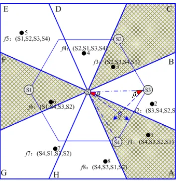
Fig. 1: Complex wireless sensor network coverage

Step1: randomly deploy N sensor nodes in monitored region of the target , through the relationship among the area of coverage, sensor nodes and the target node, from the frequent item set the target node set with the most nodes, T max is selected, and sensor node set is selected from the sensor nodes with high-energy .

Step2: remove the frequent node set that has been selected in T, and then a new target node set T1k is formed. Judge whether T1k is empty. If it is, then turn to step 5.

Step3: Let the optimal subset, calculate the coverage set and energy consumption of the concerned target node through Gaussian normal density function and probability function of coverage area, when the energy consumption is less than a specific value, return G, otherwise select the sensor nods with more energy as the overlay node.

Step4: calculate the probability of the node by using the formula (4), (5), and (6) , then initialize SN= ∅,

1

n= , '

(

)

, , , , , ,

G S T E W =G S T E W , determine whether SN is an empty set, and reset input items: G = (S, T, E, W), the

output items: optimal subset initialized, judge SN is equal to the empty set. It is not an empty set. If it’s not, setSN=SN∪Shn, n= +n 1.

Step5: determine the current energy of the sensor nodes within the target area which is covered the current sensor node, ifcn≥w, go to Step 2.

Step6: calculate to determine whether there are still target nodes not covered. If there is, then the target is covered by only one sensor node. If the target nodes are all covered, then complete coverage is achieved.

Let

(

)

N

x ,x , x⋯x be the population in the first generation of the feasible solutions individualt, Nis the population

size, t i

x denotes the first-generation t,i individuals, t i

p is Pareto superior to individual t i

x population the number

of individuals, defined as the first t i

s

(

)

i i

s =p + t t

i

x behalf of individuals ordinal values, denoted t i

x individual fitness

function tto t 1 i t i

f s

= if the first generation of Pareto superior to the more individuals t, t i

x order value is larger, the

lower the degree of its adaptation, ie individual t i

x worse quality; Contrary, adapt the higher the better the quality of the individual t

i

x .

By the uniform crossover design ideas, assume that hybridizes to two parent individuals were 1 ( 1 2 3 ) T n

p = x , x , x⋯x ,

( )

2 1 2 3

T n

p = y , y , y⋯y component of the inserted between their corresponding points, towered equally divided intoq−1:

( ) ( )

( )

1 1 1 1 1

2 2 2 2 2

2 1

2 1

2 1

n n n n n

y x , x d , x d , x q d

y x , x d , x d , x q d

y x , x d , x d , x q d

= + + + + −

 

= + + + + −

  

 _{= + + + + −}



⋯

⋯

⋯

⋯

Whered= −yi x qi −1, is the length of the corresponding component of the aliquots, as the individual components of

uniform design factor,xi+ −(q 1)d,i is the first horizontal factor of q, where q and nmust be greater than a prime

number. Uniform design method according to the previous chapter, xand ywill be generated in the hypercube formed by the quniformly distributed points, we these points asq,x and y offspring generated after the hybridization. Since the plurality of offspring in its two parent hypercube formed uniformly distributed, which is equivalent in the two parent individuals do a local search around.

According to the crossover probability of individual populations to determine whether to participate in the cross, and then a random string of individual genes set a crossover point, at the intersection of genes on arithmetic crossover operation, matching the intersection in front of the individual genes directly copied to the offspring, after the intersection after the exchange of genes assigned to the corresponding offspring. Single-point crossover complex not only maintains a simulated binary crossover advantages, but also by increasing the solving arithmetic crossover search area, enhanced search capabilities of the algorithm.

EVALUATION SYSTEM

The wireless communication models for Sensor node transmitting data and receiving data are respectively the following:

2 0 4

0

( , ) ( , )

Tr T elec amp

T elec fs T elec amp

E k d E k E k d

E k d k d d E k d k d d

ε ε

−

− −

= +

 _{+ <} 

=

+ ≥

 ₍₁₇₎

In the above formula, ET-elec and ER-elec denote the energy consumption of wireless transmitting module and wireless

receiving module; ε_{fs and} ε_{amp stand for the energy consumption parameters of spatial model and multiple attenuation}

models; d0 is a constant.

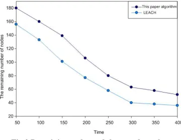
Experiment I: The first case is, with the same respective parameters, execute 50 times and get the mean value, then execute for 400 to compare with the LEACH protocol the quantitative relationship between number of remaining nodes and the number of turns, as shown in Figure 2:

Fig.2 Remaining nodes and the round number

As can be seen from Figure 2, with increasing of time, the number of remaining nodes of proposed algorithm is higher than the LEACH protocol, and then the conclusion that with the increasing of time, the energy consumption of the proposed algorithm is lower than that of LEACH protocol, and the network lifetime is extended, also the network resources are optimized.

Fig.3 Coverage rate for different coverage area

Figure 3 shows the graph of the number of sensor nodes needed to deploy to achieve different node coverage under different network dimensions. The figure shows that, with the expansion of the network, to meet the demand for network coverage, the number of nodes required to be deployed will increase, and the higher the coverage of the network, the number of nodes need to be deployed increases can be obtained from Figure more fast, so that the concern target node can achieve complete coverage.

Experiment: Figure 4 shows a diagram of the number of sensor nodes need to be deployed for the same network size 400*400m2 under different node coverage requirement, and compare with the experiments of literature SCCP algorithm, to meet certain demand for network coverage, the number of nodes deployed will be gradually increased as time progresses, and the network coverage will also increase, so that completely coverage is achieved for the same coverage area and different nodes coverage for target area, as shown in figure4:

Fig.4: Coverage comparison of proposed algorithm and SCCP

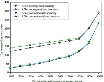
Fig.5 Curves of network coverage rate

required increases substantially; and the influences gradually become smaller and in equilibrium at last when the network coverage and connectivity rate increases.

Fig.5 reflects the number of nodes required to be deployed to achieve different coverage and connectivity rates without the boundary influence. Compared with the boundary influence, the number of nodes deployed increases slightly, and with the increase of nodes, node density will become larger, so the boundary influence becomes lower.

CONCLUSION

The main task of multi-objective optimization is to improve the quality of the solution and maintain the solution of a broad distribution and uniformity, the weighted sum genetic algorithm is a straightforward, practical, strong multi-objective genetic algorithms. This paper focuses on the weighted sum of the genetic algorithm, uniform design created by combining the initial population, and their respective objective function Number of standardization, the establishment of a new fitness function, and proposes a dynamic allocation weighting scheme, designed a new weight-based allocation strategy Multi-objective Genetic Algorithm for multi-objective optimization problem. Second, the design of a uniform design method based on multi-objective optimization genetic algorithm, and gives a proof of convergence of the algorithm by simulation to verify the effectiveness of the algorithm. In this paper, the Gaussian normal density function and probability function of the coverage area are adopted to optimized set of sensor nodes to form a minimal subset and determine the maximum target set, by state transition of sensor nodes, nodes enter different states, work in turn, thus network energy consumption is saved , network lifetime is extended, the ratio of network resources and quality of service is improved, also redundant nodes are reduced, and last, the network performance is optimized. Finally, through simulation, the effectiveness and stability of the algorithm are verified, due to the presence of vast network throughput and constrain by external factors, amativeness to very large sensor network is the next focus of the study subject.

Acknowledgments

The authors wish to thank Science of Technology Research of Foundation Project of Henan Province Education Department under Grant Nos.2014B520099; Natural Science and Technology Research of Foundation Project of Henan Province Department of Science under Grant Nos. 142102210471.

REFERENCES

[1]Zou Y and Charrabarty K. Ad Hoc Network v.11, n.2, pp.286-297, February, 2003. [2]Schuragers C, Tsiatsis V. IEEE Trans. Mobile computer, v.1, n.1, pp 70-80, January 2002. [3]Thomas.H Y, Shi Y. IEEE/ACM Trans. Networking, v.16, n.2, pp.321–334, February, 2008. [4]Jiang J, Fang L. Journal of Software, v.17,n.2, pp. 175-184, February, 2006.

[5]Salabat K, Mohsin B. International of Artificial Intelligence, V.7,n.11,pp.198-207, November,2008 [6]Cardei M, Ding Z D. Wireless Networks,V.3, n.11,pp.333-440. November, 2005

[7]Ayoub B, Mohammad R. Journal of Artificial Intelligence, V.8, n.1, pp.86-95, January, 2008 [8]Jie W, Fei D. Journal of Communications and Networks,V.1,n.4, pp.1-12, April, 2002 [9]Salcedo S, Xin Y. IEEE Transactions on Systems.V.3,n.5, pp.2343-2353, May, 2004