Investigating the impact of distributed generators power factor to simultaneous optimization analysis

Investigating the Impact of Distributed Generators Power Factor to

Simultaneous Optimization Analysis

J. J. Jamian

,

M. W. Mustafa

and M. N. Abdullah

1

Faculty of Electrical Engineering, Universiti Teknologi Malaysia,81310 UTM Johor Bahru, Malaysia

2_{Faculty of Electrical and Electronic Engineering, Universiti Tun Hussien Onn Malaysia, 86400}

Johor, Malaysia a

[email protected], [email protected], [email protected]

Keywords: Distribution System, Simultaneous Analysis, Optimal DG Coordination, Power Factor, Power Loss

Abstract. In this paper, the Particle Swarm Optimization (PSO) technique is used to determine the optimal coordination for Distributed Generator (DG). The DG output and location is determined simultaneously. Furthermore, this study covers both single and multiple DGs analyses. Five different Power Factor (PF) values are also assigned to the DG units, which are 0.8, 0.85, 0.9, 0.95 and 1.0. Thus, the impacts of DG power factor to the optimal placement and output are investigated. From the result, the optimal DG placement is similar, regardless of the PF condition. For the single DG unit, the optimal location is bus 6 and for three DGs analysis, the optimal locations are at buses 14, 24, 30. However, the PF significantly influences the optimal DG output, power loss reduction and voltage profile improvement. Three DGs with PF 0.8 is the best option to reduce the power loss in the distribution network to the lowest value.

Introduction

Distribution network is one of the main components in electric power system that supplies power to the end user, either to industrial areas or residential areas. Originally, the distribution network is operated passively. This means that power supplied by the network totally depended on transmission/distribution substation. However, the introduction of Distribution Generator (DG) has transformed the behavior of the distribution network into an active system [1,2,3,4]. With the DG implementation, some of the load will be supplied by DG and remaining loads are supplied by existing substations.

However, it is very important to ensure that the DG location and their generated power are configured properly. Without proper placements, the DG will not be able to reduce the power loss to the lowest value [5,6]. Moreover, the non-optimal DG output can cause higher power loss than the initial condition and in the worst case, it could cause the distribution system to collapse. Therefore, many studies on optimal DG output and placement have been done [7,8,9].

Murthy et. al. [10], for example, have proposed the optimal DG based on sensitivity approach. The proposed sensitivity technique has given better DG placement and size compared to other existing indices, such as combined loss sensitivity, index vector, and voltage sensitivity index. Furthermore, the power loss in the system is also reduced. On the other hand, other approaches on optimal DG placement have been proposed by Lee et. al. [11]. The authors used power loss sensitivities or known as optimal locator index as a guidance to determine suitable DG location. The Kalman Filter technique is used for determining the suitable size of DG with the step increment of 10 kW.

Power Factor (PF) condition, which are PF = 0.8, PF = 0.85, PF = 0.90, PF = 0.95 and PF = 1.0. Thus, the investigation on the impact of PF as well as number of DG will be discussed in detail. The 33-bus radial distribution system is selected as the test case system.

Problem Formulation

The installation of DG in the distribution network is capable of reducing the existing power loss and improving the voltage profile. However, the improvement depends on the appropriate DG coordination. In this paper, the PSO algorithm is used to solve the single and multiple DG coordination problems. The power loss value could be in the minimum value by finding the optimal DG location and output. The power loss, which is set as the objective function is calculated using (1).







j j j

Loss

I

R

P

max

1 2

(1)

Besides that, several constraints are considered in the analysis in order to make the solution feasible and close to actual practical system. The lists of constraints are:

i. DG output power:

max min

i DGi

i

P

P

P





 





P

Q_DGi  _DGi tancos1 (3)

The randomization and updating value for DG output, which is given by PSO algorithm, must be within the DG capability limit. The DG output should not be lower than the minimum DG rated or higher than the maximum DG rated as shown in (2). Besides that, since the DG operates at a specific PF value, the reactive power supplied by the DG is equal to (3).

ii. Power Injected Constraint:

Losses Load

DG of no

h DG

P P P

h  



.

1

(4)

The total power supplied by DGs to the system must be less than the total amount of demand and total power loss value. The purpose of this restriction is to avoid any power injection to the grid side.

iii. Power balance constraint:

Losses Load

Substation DG

of no

h

DG P P P

P _h   





.

1

(5)

iv. Voltage Constraint:

max

min V V

V  _bus  (6)

The voltage value at any bus in the system should be better than initial condition after the DG installation, either for single or multiple DG cases. Besides that, the voltage value should not

exceed the maximum allowable limit (Vmax), which is 1.05p.u and should be higher than the

minimum allowable limit (Vmin), which is 0.95p.u.

Therefore, all these constraints will be checked every time the updating process is done in the PSO algorithm. If the result of placement and DG output caused violation in any of the constraints, the PSO will add the penalty value to the objective function. The test system and PSO algorithm were conducted using MATLAB programming language in MATLAB 7.8 with 2GB RAM.

Particle Swarm Optimization Implementation

Particle Swarm Optimization (PSO) algorithm is a technique proposed by Ebehart and Kennedy [12] and has been widely used in many applications such as in engineering field and financial problem. The idea of PSO is adapted from the food searching behavior of birds or fish. In optimization process, the birds or fish is known as particles. These particles will move with a specific guidance and change their position and speed until they arrive at the destination, which is known as food source location.

Furthermore, the changes in new position and new speed of each particle depend on their own information (local best - Pbest) and others (global best - Gbest). In general, the updated formulae to find the new velocity and new position for the particles proposed by Yuhui and Ebehart [13] are:

)

(

)

(

1 1

1 k

i k best i k

i k

i best i k i k

i k

i

v

c

r

P

x

c

r

G

x

v













k i k

i k

i

v

x

x





where:

ω = Inertia weight of particle

υ = Velocity of particle

c1, c2 = Acceleration constant (cognitive and social)

r1, r2 = Random number between ‘0’ to ‘1’

Pbest = The best fitness that given by particle until current iteration

Gbest = The best fitness that given by any particles in the population at current iteration

The inertia weight (ωi) value is different in each iteration and based on the following equation:



_{  }

k k

i

max min max

max









where:

k = Iteration number













i rand DG ceil rand DG

x  (10)

Thus, the location and output will be updated simultaneously in the PSO process until the maximum iteration is reached. Fig. 1 shows the flow chart of PSO algorithm in solving the simultaneous DG placement and output problem based on PF condition.

Start

Randomize the position (DG location and output) and calculate the power loss of each particle (yi)

Determine Pbest and Gbest value for

1st _{iteration (k=1)}

Fulfill all the constraints?

Calculate the new DG location and output, xik+1 and velocity, vik+1

Determine the new power loss of each particle, yik+1

Find Pbest and Gbestvalues for next iteration

by comparing previous (k) and current power loss (k+1) value

yi+1(max)- yi+1(min) = ε?

Iteration = max value?

k=k+1

END

No No

Yes Yes

Yes Yes

No No Set the number, N& initial velocity, v

of particles

Re-generate New random position (xi)

Calculate reactive power injected by DG based on power

factor and DG output value

Calculate reactive power injected by DG based on power factor and new DG output value

Fig.1: The process to find the optimal DG placement and output

Particle Swarm Optimization Implementation

The original 33 bus system, as shown in Fig. 2, is a radial distribution system with total load of 3.715 MW, 2.3 MVar and the real loss in the system is 203.18 kW. Besides that, the PSO parameters that being set in this study are:

• c1 = c2 = 1.4;

• ωmin = 0.9;

• ωmax = 0.4;

• N = 20;

Fig. 2: The case study network: 33-bus radial distribution system

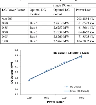
Table 1 shows the optimal DG location and output based on the PF value for single DG analysis. From the results, the optimal location for DG is similar regardless of the PF condition, which is at bus 6. However, the PF affects the power loss and total optimal DG output results. From the analysis, the power loss value is between 60 kW to 72 kW when the DG is operated at 0.8 to 0.95 PF and double up to 104.38 kW when the DG is operated at PF 1.0. In term of optimal DG operation, the amount of output is increasing when the DG is operated from 0.8 (PF) to 0.95 (PF). The increment can be presented as a linear equation as shown in Fig. 3. In a nutshell, the PF does not only affect the power loss value, it also affects the DG output.

Table 1: Optimal DG Location and Output for Single DG Unit

Single DG unit

DG Power Factor Optimal DG

location

Optimal DG output

Power Loss

w/o DG - - 203.1854 kW

0.80 Bus 6 2.4719 MW 61.6523 kW

0.85 Bus 6 2.6257 MW 61.7661 kW

0.90 Bus 6 2.7534 MW 64.4667 kW

0.95 Bus 6 2.8269 MW 71.8595 kW

1.00 Bus 6 2.5762 MW 104.3802 kW

DG_output = 0.1418(PF) + 2.6289

2.5 2.6 2.7 2.8 2.9 3.0 3.1 3.2 3.3

0.80 0.85 0.90 0.95

DG

Out

put

(

MW)

Power Factor

DG Output Linear (DG Output)

Fig. 3: The relationship between optimal DG output and PF value

2 3 4 5 6 7 8 9 10 11 12 13 14 15 16 17 18

19 20 21 22

26 27 28 29 30 31 32 33

23 24 25

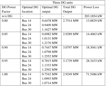
Further power loss reduction can be obtained when multiple DGs are placed in the network. However, similar to the single DG analysis, the optimal locations for multiple DGs are the same and are not affected by the PF value as shown in Table 2. The DG must be located at buses 14, 24 and 30 in order to get the lower power loss and the PF 0.8 gives the lowest power loss in the system compared to the others.

Table 2: Optimal DG Location and Output for Multiple DG Units

Three DG units DG Power

Factor

Optimal DG location

Optimal DG output

Total DG Output

Power Loss

w/o DG - - - 203.1854 kW

0.80 Bus 14

Bus 24 Bus 30

0.6478 MW 0.9409 MW 1.1627 MW

2.7514 MW 13.8829 kW

0.85 Bus 14

Bus 24 Bus 30

0.6982 MW 1.0131 MW 1.2176 MW

2.9289 MW 14.4063 kW

0.90 Bus 14

Bus 24 Bus 30

0.7447 MW 1.0798 MW 1.2552 MW

3.0797 MW 18.3041 kW

0.95 Bus 14

Bus 24 Bus 30

0.7815 MW 1.1333 MW 1.2592 MW

3.1739 MW 28.3433 kW

1.00 Bus 14

Bus 24 Bus 30

0.7542 MW 1.0993 MW 1.0714 MW

2.9249 MW 71.5486 kW

In terms of total output, the spreading of DG in the system causes the total optimal DG output to become larger than a single DG output. For example, the total DG output given by PF 0.85 is 2.6257 MW for single DG and 2.9289 MW for three DGs. There is an addition of 11.55% of active power provided by three DGs analysis. Therefore, the reactive power that will be supplied to the system is also increased as shown in Fig. 4.

0 10 20 30 40 50 60 70 80

0.80 0.85 0.90 0.95 1.00

11.31 11.55 11.85 12.27

0.00 77.48 76.68

71.61

60.56

31.45

Per

cen

tag

e

(%)

Power Factor

Additional Mvar (3 DGs) Addition Power Loss Reduction (3 DGs)

Although additional reactive power is required for 3 DGs case (except for PF 1.0), the reduction of power loss is very large compared to single DG configuration. From the figure, when the DG operates at PF 0.8, the power loss for 3 DGs configuration in the system is 77.48% lower than single DG configuration. The deviation between these two conditions is calculated based on the following equation:





_

_

result 

 (11)

Thus, from the bar chart, the distribution network performance is much better under multiple DG installation.

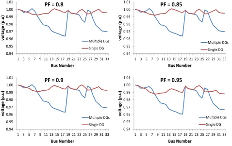
The voltage profile of the system was also improved tremendously by the reactive power injection. Fig. 5 shows the comparison of voltage profile after the DG installation for all PF conditions. From the results, there are certain bus voltages given by 3 DGs are lower than single DG, such as buses 4, 5 and 6. However, the placement of 3 DGs was able to ensure that all buses were operated above 0.98p.u. The small variation in voltage profile, indirectly, will reduce the amount of current flow in the line, which causes power loss reduction in the system (P=I2R). Therefore, it can be concluded that multiple DGs can provide better performance to the radial distribution system. 0.94 0.95 0.96 0.97 0.98 0.99 1.00 1.01

1 3 5 7 9 11 13 15 17 19 21 23 25 27 29 31 33

voltag

e

(p.u)

Bus Number

PF = 0.8

Multiple DGs Single DG 0.94 0.95 0.96 0.97 0.98 0.99 1.00 1.01

1 3 5 7 9 11 13 15 17 19 21 23 25 27 29 31 33

voltag

e

(p.u)

Bus Number

PF = 0.85

Multiple DGs Single DG 0.94 0.95 0.96 0.97 0.98 0.99 1.00 1.01

1 3 5 7 9 11 13 15 17 19 21 23 25 27 29 31 33

voltag

e

(p.u)

Bus Number

PF = 0.9

Multiple DGs Single DG 0.94 0.95 0.96 0.97 0.98 0.99 1.00 1.01

1 3 5 7 9 11 13 15 17 19 21 23 25 27 29 31 33

voltag

e

(p.u)

Bus Number

PF = 0.95

Multiple DGs Single DG

Fig. 5: The comparison of voltage profile provided by single and multiple DGs

Conclusion

the total DG output for multiple DG unit is quite larger than single DG analysis, the spreading of DG help tremendously in improving the voltage profile. Thus, the particle swarm optimization has worked perfectly in finding the optimal DG placement and output, in order to improve the distribution system performance.

Acknowledgement

The researchers would like to express their appreciation to the University Teknologi Malaysia (UTM) and Ministry of Higher Education (MOHE) for funding this research.

References

[1] T. N. Shukla, S. P. Singh, V. Srinivasarao, K. B. Naik, Optimal Sizing of Distributed Generation Placed on Radial Distribution Systems, Electric Power Components and Systems, 38 (2010) 260-274.

[2] A. Soroudi, M. Ehsan, Efficient immune-GA method for DNOs in sizing and placement of distributed generation units, European Transactions on Electrical Power, 21 (2011) 1361-1375.

[3] M. Afkousi-Paqaleh, A.A.T. Fard, M. Rashidinejad, Distributed generation placement for congestion management considering economic and financial issues, Electrical Engineering, 92 (2010) 193-201.

[4] R. K. Singh, S. K. Goswami, Optimum Siting and Sizing of Distributed Generations in Radial and Networked Systems, Electric Power Components and Systems, 37 (2009) 127-145.

[5] F. S. Abu-Mouti, M. E. El-Hawary, Heuristic curve-fitted technique for distributed generation optimisation in radial distribution feeder systems, IET Generation, Transmission and Distribution, 5 (2011) 172-180.

[6] L. Zhipeng, W. Fushuan, G. Ledwich, J. Xingquan, Optimal sitting and sizing of distributed generators based on a modified primal-dual interior point algorithm, 4th International Conference on Electric Utility Deregulation and Restructuring and Power Technologies, (2011) 1360-1365.

[7] V. Veeramsetty, G.V.N. Lakshmi, A. Jayalaxmi, Optimal allocation and contingency analysis of embedded generation deployment in distribution network using genetic algorithm, International Conference on Computing, Electronics and Electrical Technologies, (2012) 86-91.

[8] K.M. Sharma, K.P. Vittal, A heuristic approach to distributed generation source allocation for electrical power distribution systems, Iranian Journal of Electrical and Electronic Engineering, 6 (2010) 224-231.

[9] V.K. Shrivastava, O.P. Rahi, V.K. Gupta, S.K., Singh, Optimal location of distribution generation source in power system network, IEEE 5th Power India Conference, (2012) 1-6.

[10] V.V.S.N. Murthy, A. Kumar, Comparison of optimal DG allocation methods in radial distribution systems based on sensitivity approaches, International Journal of Electrical Power & Energy Systems, 53 (2013) 450-467.

[11] S.H. Lee, J.W. Park, Optimal Placement and Sizing of Multiple DGs in a Practical Distribution System by Considering Power Loss, IEEE Transactions on Industry Applications, 49 (2013) 2262-2270.

[12] J. Kennedy, R. Eberhart, Particle swarm optimization, IEEE International Conference on Neural Networks Proceedings, (1995) 1942-1948.