BIROn - Birkbeck Institutional Research Online
Zhang, Dell and Wang, Jun and Yilmaz, Emine and Wang, Xiaoling and
Yuxin, Zhou (2016) Bayesian performance comparison of text classifiers.
In: UNSPECIFIED (ed.) Proceedings of the 39th International ACM SIGIR
Conference on Research and Development in Information Retrieval (SIGIR).
New York, U.S.: Association for Computing Machinery, pp. 15-24. ISBN
9781450340694.
Downloaded from:
Usage Guidelines:
Please refer to usage guidelines at
or alternatively
Bayesian Performance Comparison of Text Classifiers
Anonymous Authors
ABSTRACT
How can we know whether one classifier is really better than the other? In the area of text classification, since the publi-cation of Yang and Liu’s seminal SIGIR-1999 paper, it has become a standard practice for researchers to apply null-hypothesis significance testing (NHST) on their experimen-tal results in order to establish the superiority of a classifier. However, such a frequentist approach has a number of inher-ent deficiencies and limitations, e.g., the inability to accept the null hypothesis (that the two classifiers perform equally well), the difficulty to compare commonly-used multivariate performance measures likeF1scores instead of accuracy, and so on. In this paper, we propose a novel Bayesian approach to the performance comparison of text classifiers, and ar-gue its advantages over the traditional frequentist approach based ont-test etc. In contrast to the existing probabilistic model forF1 scores which is unpaired, our proposed model takes the correlation between classifiers into account and thus achieves greater statistical power. Using several typical text classification algorithms and a benchmark dataset, we demonstrate that the our approach provides rich information about the difference between two classifiers’ performances.
Categories and Subject Descriptors
H.3.4 [Information Storage and Retrieval]: Systems and Software—performance evaluation (efficiency and effec-tiveness); I.5.2 [Pattern Recognition]: Design Methodol-ogy—classifier design and evaluation
Keywords
Text Classification; Performance Evaluation; Hypothesis Test-ing; Bayesian Inference
1.
INTRODUCTION
Text classification (aka categorisation) [30] is a fundamen-tal technique in information retrieval (IR) [21]. It has many important applications, including topic categorisation, spam
Permission to make digital or hard copies of all or part of this work for personal or classroom use is granted without fee provided that copies are not made or distributed for profit or commercial advantage and that copies bear this notice and the full cita-tion on the first page. Copyrights for components of this work owned by others than ACM must be honored. Abstracting with credit is permitted. To copy otherwise, or re-publish, to post on servers or to redistribute to lists, requires prior specific permission and/or a fee. Request permissions from [email protected].
SIGIR ’16 Pisa, Italy
c
2016 ACM. ISBN 123-4567-24-567/08/06. . . $15.00
DOI:10.475/123 4
filtering, sentiment analysis, message routing, language iden-tification, genre detection, authorship attribution, and so on. In fact, most modern IR systems for search, recommenda-tion, or advertising contain multiple components that use some form of text classification.
How can we know whether one classifier is really better than the other? Is it possible that they perform equally well? Sure we should be able to evaluate their classification performances on some benchmark datasets using some per-formance measures. However, given any finite amount of test results, we can never be completely certain that one classi-fier works better than the other or vice versa: the observed difference between their performance scores do not neces-sarily reflect their intrinsic qualities. The central question here is how to reliably tell if classifier A indeed outperforms classifier B, given a set of test results. Perhaps the simplest solution is to applyk-fold cross-validation [24] and then cal-culate the sample variance of performance scores over mul-tiple “folds” of the dataset. This method tends to yield poor estimations though: the sample variance can approximate the true variance well only if we have a large number of folds, but when the dataset is divided into many folds, the size of each fold is likely to be too small to give a meaning-ful performance score (especially for complex multivariate performance measures likeF1[31]). Hence it is desirable to derive the uncertainty of performance scores directly from all the atomic document-category classification results.
To address this problem, Yang and Liu defined in their seminal SIGIR-1999 paper [34] a suite of null-hypothesis sig-nificance testing (NHST) methods which aim to verify how strongly the experimental results support the claim that one particular classifier is more accurate than another classifier. That paper has been influential within and beyond the realm of text classification. Since its publication, it has received about 3,000 citations (according to Google Scholar). Today, it is almost compulsory for researchers to validate the su-periority of their proposed text classification algorithms by means of NHST and report thep-values in their papers.
provides rich information about the difference between two classifiers’ performances.
2.
RELATED WORK
2.1
Frequentist Performance Comparison
The traditional frequentist approach to comparing clas-sifiers is to use NHST [24]. The usual process of NHST consists of four steps: (1) formulate the null hypothesisH0 that the observations are the result of pure chance and the alternative hypothesisH1 that the observations show a real effect combined with a component of chance variation; (2) identify a test statistic that can be used to assess the truth of
H0; (3) compute thep-value, which is the probability that a test statistic equal to or more extreme than the one observed would be obtained under the assumption of hypothesisH0; (4) if thep-value is less than an acceptable significance level, the observed effect is statistically significant, i.e.,H0is ruled out andH1 is valid.
Specifically for performance comparison of text classifiers, the usage of NHST has been presented in detail by Yang and Liu in their SIGIR-1999 paper [34]. In summary, on the doc-ument level (micro level), sign-test can be used to compare two classifiers’ accuracy scores (called s-test), while unpaired
t-test can be used to compare two classifiers’ performance measures in the form of proportions, e.g., precision, recall, error, and accuracy (called p-test); on the category level (macro level), sign-test and pairedt-test can both be used to compare two classifiers’F1 scores [31] (which are called S-test and T-test respectively).
In spite of being useful and influential, such a frequen-tist approach unfortunately has many inherent deficiencies and limitations [17, 18]. First, NHST is only able to tell us whether the experimental data are sufficient to reject the null hypothesis (that the performance difference is zero) or not, but there is no way to accept the null hypothesis. If we fail to reject the null hypothesis, we cannot conclude that it is true, but only recognise that the null hypothesis is a pos-sibility. That is to say, it is impossible for us to use NHST to confidently claim that two classifiers perform equally well . Second, NHST will reject the null hypothesis as long as the experimental data suggest that the performance difference is non-zero, even if the performance difference is too slight to have any real effect in practice. Third, complex performance measures such as theF1score can only be compared on the category level but not on the document level, which seri-ously restricts the statistical power of NHST as the number of categories is usually much much smaller than the number of documents. Fourth, using unpaired t-test, the correla-tion between the classifiers in comparison are totally ignored, which is unreasonable because in reality both classifiers are likely to do well on “easy” test documents, and badly on “dif-ficult” test documents, not to mention that those classifiers could be just different versions of the same machine learn-ing algorithm. Fifth, uslearn-ing sign-test, those pairs of identical classification outcomes are completely discarded, which is undesirable because the probability that the two classifiers are essentially equal would be substantially underestimated. Sixth, complicated corrections would be needed if the com-parison is extended to multiple classifiers.
The other NHST methods that have been applied to com-pare classifiers include ANOVA test [14], Friedman test [29], McNemar’s test [9], and Wilcoxon signed ranks test [6]. Due
to their frequentist nature, no matter which specific test they use, more or less they suffer from the above mentioned perils (especially the first three).
2.2
Bayesian Performance Comparison
It has been loudly advocated in recent years that the Bayesian approach to comparing two groups of data has many advantages over the frequentist NHST [17, 18]. How-ever, to our knowledge, almost all the existing models of Bayesian performance comparison deal with continuous val-ues (that can be described by Gaussian or tdistributions) but not discrete classification outcomes, and they produce estimations for simple statistics (such as the average differ-ence between the two given groups) but not complex perfor-mance measures (such as theF1 score). Probably the most closely related work is that of Goutte and Gaussier [12]. TheirF1 score model constructed using a couple of Gamma variates is not as expressive and flexible as ours. In con-trast, our proposed approach opens up many possibilities for adaptation or extension. Furthermore, the two groups of data are assumed to be independent with each other, which is usually reasonable for applications like medical trails or psychological experiments but does not make much sense for our task of comparing two classifiers. Our experiments re-veal that such an “unpaired” model ignoring the correlation between classifiers has much lesser statistical power than the “paired” model (see Section 4.1).
3.
OUR APPROACH
3.1
Probabilistic Models
Let us consider a text classifier which has been tested on a collection ofN labelled test documents, D. For each documentxi (i= 1, . . . , N), we have its true class labelyi as well as the predicted class label ˆyi.
If this classifier is actually a Bayesian model, in princi-ple there should be a direct way to assess the suitability of modelMin explaining the experimental data by computing Pr[M|D] ∝ Pr[M]R
ΘPr[D|Θ,M] Pr[Θ|M]dΘ. However, here we would like to consider the general situation where the true and predicted class labels are the only information presumed to be available.
In the most basic setting, binary classification, a docu-ment belongs to either the positive class or the negative class. Without loss of generality, we use integer 1 as the ID of the positive class and integer 0 as the ID of the negative class. Furthermore, for the sake of clarity, we will also denote the true positive and negative classes using notations+and
−respectively which should be regarded as interchangeable synonyms of class IDs 1 and 0.
The test documents can usually be considered as “inde-pendent trials”, so we regard both their true class labelsyi and their predicted class labels ˆyias independent and iden-tically distributed (i.i.d.) random variables.
Table 1: The classification results from one binary classifier.
yi yˆi
+ µ 1 ρ
+
0 1−ρ+
− 1−µ 1 ρ −
0 1−ρ−
Given a test documentxi, we useµto represent the prob-ability that its true class labelyiis positive. Obviously the probability that yi is negative would therefore be 1−µ. This means thatyifollows a Bernoulli distribution with pa-rameterµ: yi∼Bern(µ), i.e., Pr[yi|µ] =µyi(1−µ)1−yi. It would then be convenient to use the Beta distribution (which is conjugate to the Bernoulli distribution) as the prior dis-tribution of parameterµ. More specifically, µ ∼Beta(β),
i.e., Pr[µ] = Γ(βΓ(β++)Γ(β,β−−))µ
β+−1
(1−µ)β−−1 where the hyper-parameterβ= (β+, β−) encodes our prior belief about each class’s proportion. If we do not have such knowledge, we can simply setβ= (1,1) that yields a uniform distribution, as we did in our experiments.
When a test documentxiwith true class labelyiis clas-sified, we anticipate that it will be classified as positive with a certain probability ρyi, i.e., Pr[ˆy
i = 1|ρyi] = ρyi. For example, ρ− is the probability that a negative (−) docu-ment is classified to be positive (1). Hence we can say that ˆ
yifollows a Bernoulli distribution with parameterρ+ when
yi is positive andρ− when yi is negative. In other words, ˆ
yi ∼ Bern(ρ+) if yi = + and ˆyi ∼ Bern(ρ−) if yi = −. It would then be convenient to use the Beta distribution as the prior distribution of parameterρ+andρ−. More
specifi-cally,ρ+∼Beta(α+), i.e., Pr[ρ+] = Γ(α + 1,α
+ 0) Γ(α+1)Γ(α+0)ρ
+α+1−1 (1−
ρ+)α+0−1 where the hyper-parameter α+ = α+ 1, α
+ 0
en-codes our prior belief about the classifier’s prediction accu-racy on positive test documents. In the same way, we have
ρ−∼Beta(α−), whereα−= α−1, α
−
0
. If we do not have any prior knowledge, we can simply setα+ =α−
= (1,1) that yields a uniform distribution, as we did in our experi-ments.
Once the parametersµ,ρ+andρ−have been estimated, it will be easy to calculate the contingency table of “expected” classification results: true positive (tp), false positive (f p), true negative (tn), and false negative (f n). For example, the anticipated number of true positive predictions of the clas-sifier should be the number of positive test documentsN µ
times the rate of being predicted by the classifier as positive
ρ+. The equations to calculate the contingency table for a classifier are listed as follows.
tp=N µρ+ f p=N(1−µ)ρ−
f n=N µ(1−ρ+) tn=N(1−µ)(1−ρ−)
With the contingency table for a classifier available, we can compute not only the accuracy, but also more complex performance measures such as theF1score for that classifier. The precisionP, recallR, and their harmonic meanF1score could be computed as follows.
P = tp
tp+f p =
µρ+
µρ++ (1−µ)ρ−
N
β
µ
ρ−
ˆ yi
yi
ψ
ρ+ α−
α+
(a) original
µ
n+ c+ n−
ψ
β
ρ−
N
ρ+ α−
c−
α+
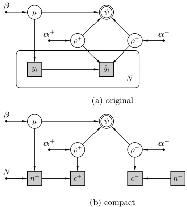
[image:4.612.344.525.490.573.2](b) compact
Figure 1: The probabilistic graphical model for a binary text classifier’s performance.
R= tp
tp+f n=
µρ+
µρ++µ(1−ρ+) =ρ +
F1= 2P R P+R
It can be seen thatN is cancelled out in the calculation of the precision, the recall, and theF1 score.
Such a model is quite general to accommodate various performance measures (see Section 5), though in this paper we focus on theF1 score only to illustrate the usage of our model. Letψdenote the chosen performance measure, then it is simply a function that depends on µ,ρ+ andρ−
only:
ψ=f(µ, ρ+, ρ−
).
This model describes a generative mechanism of a clas-sifier’s test results. It is summarised as follows, and also depicted in Figure 1a as a probabilistic graphical model (PGM) [16] using common notations.
µ ∼Beta(β)
yi ∼Bern(µ) fori= 1, . . . , N
ρ+∼Beta(α+) ρ−∼Beta(α−)
ˆ
yi ∼
(
Bern(ρ+) fori= 1, . . . , N ify i=+ Bern(ρ−) fori= 1, . . . , N ifyi=−
ψ =f(µ, ρ+, ρ−)
In the above model, each true class labelyi is regarded as an individual sampling event, and each prediction ˆyi is treated as an individual sampling event too. If we aggre-gate the occurrences of such individual sampling events into the counts of their occurrences, the model could be greatly simplified.
Let n+ represent the total number of positive test doc-uments and n− = N−n+ represent the total number of negative test documents, then n+ is known to follow the Binomial distribution with parameters N and µ: n+ ∼ Bin(N, µ), i.e., Pr[n+|N, µ] = nN+
µn+(1−µ)N−n+ where N
n+
= N!
n+!(N−n+)! is the Binomial coefficient.
produced on positive test documents (yi = +), then c+ is known to follow the Binomial distribution with param-etersn+ and ρ+: c+ ∼Bin(n+, ρ+), i.e., Pr[c+|n+, ρ+] =
n+ c+
ρ+c+(1−ρ+)n+−c+. In the same way, we have c− ∼
Bin(n−, ρ−).
The parametersµ,ρ+ andρ−
are the same as before and their prior distributions remain the same. The deterministic variableψalso stays unchanged.
This compact model is equivalent to the original model, but it will be computationally much more efficient due to the drastic reduction of sampling events. So hereafter the compact model will be used instead of the original model for our work on performance comparison.
The compact model is summarised as follows and depicted in Figure 1b.
µ ∼Beta(β)
n+∼Bin(N, µ) n−=N−n+ ρ+ ∼Beta(α+) ρ−∼Beta(α−)
c+ ∼Bin(n+, ρ+) c−∼Bin(n−, ρ−)
ψ =f(µ, ρ+, ρ−)
The usage of conjugate priors (e.g., Beta for Bernoulli or Binomial) is not obligatory in our model. Actually any rea-sonable probability distribution can be used as the prior of
µ,ρ+orρ−. If we insist on using conjugate priors, it is pos-sible to simplify the model even further by computing the posterior probability distributions of our model parameters analytically and then sampling from the posterior probabil-ity distributions directly. However, this will only bring mod-erate improvement to computational efficiency, and more importantly it will make the model less flexible as some ex-tensions to the model (such as hierarchical modelling) will be obstructed. So we shall not go down that direction in this paper.
3.1.1
Unpaired Model
In the unpaired model for performance comparison, the two classifiers A and B to be compared are assumed to be independent with each other [12, 35, 36]. They could even be evaluated on different test datasets as long as they come from the same data distribution (e.g., with the same propor-tion of positive test examples). So we can simply pool the two probabilistic models for those two classifiers together, and introduce a deterministic variableδ to capture the dif-ference between their performance scoresψA andψB.
δ=ψA−ψB
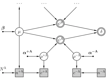
The unpaired model consisting of two separate sub-models for two classifiers A and B is depicted in Figure 2, where most of the sub-model for B is omitted as it is symmetric to that of A.
3.1.2
Paired Model
Although the unpaired model is simple and effective, its underlying assumption that the predictions from two clas-sifiers A and B are independent of each other is unrealistic when those two classifiers are evaluated on the same test dataset. In contrast to the existing work for classification performance comparison (see Section 2), we would like to avoid this unrealistic assumption by modelling the two clas-sifiers’ predictionsjointlyas pairs. This is indeed crucial to
· · ·
µ
n+A
ψB
n−A
c+A
ψA
β
ρ−A
NA
· · · ·
ρ+A
δ
α−A
c−A
[image:5.612.326.511.56.192.2]α+A
Figure 2: The unpaired model for performance comparison.
ψA
β
ψB
α−
N
c− n−
δ
θ− α+
µ
n+ c+
[image:5.612.324.512.221.329.2]θ+
[image:5.612.362.510.384.508.2]Figure 3: The paired model for performance comparison.
Table 2: The classification results from two binary classifiers.
yi yˆiA yˆBi oi
+ µ
1 1 (1,1) θ+(1,1)
1 0 (1,0) θ+(1,0)
0 1 (0,1) θ+(0,1)
0 0 (0,0) θ+(0,0)
− 1−µ
1 1 (1,1) θ−(1,1)
1 0 (1,0) θ−(1,0)
0 1 (0,1) θ−(0,1)
0 0 (0,0) θ−(0,0)
assessing the real significance of the two classifiers’ perfor-mance difference, as we demonstrate later in our experiments (see Section 4.1).
Considering two classifiers A and B evaluated on the same document collection, we have for each document xi (i = 1, . . . , N) a prediction outcome pair oi = (ˆyAi,yˆ
B i) where ˆ
yiAand ˆyiBare the predicted class labels given by A and B respectively.
Table 2 lists all the possible classification results and their corresponding probabilities for a test document using two binary classifiers. Since for each of the two possibleyivalues there are four possibleoivalues{(1,1),(1,0),(0,1),(0,0)}, this table has 2×4 = 8 entries in total.
When a test documentxiwith true class labelyiis clas-sified by the two classifiers A and B, we anticipate that each possible prediction outcome pairoiwill occur with a certain probabilityθyi
oi, i.e., Pr[oi|θ
yi] =θyi
to be negative (0) by the classifier A and positive (1) by the classifier B. If we letθ+ denote the vector of parame-tersθo+iand similarly letθ
−
denote the vector of parameters
θo−i, then we can say thatoifollows a Categorical distribu-tion with parameter θ+ when yi is positive andθ− when
yi is negative. In other words, oi ∼ Cat(θ+) if yi = + and oi ∼ Cat(θ−) if yi = −. It would then be conve-nient to use the Dirichlet distribution (which is conjugate to the Categorical distribution) as the prior distribution of pa-rameterθ+ or θ−. More specifically, θ+ ∼ Dir(α+), i.e.,
Pr[θ+] = Γ(Pkα+k)
Q
kΓ(α+k)
Q
kθ α+k−1
k where the hyper-parameter
α+ = α+(1,1), . . . , α+(0,0) encodes our prior belief about the classifier’s prediction accuracy on positive test docu-ments. In the same way, we have θ− ∼ Dir(α−), where
α− = α−(1,1), . . . , α−(0,0). If we do not have any prior knowledge, we can simply set α+ = α− = (1, . . . ,1) that yields a uniform distribution, as we did in our experiments.
Letc+=c+
(1,1), . . . , c + (0,0)
represent the counts of differ-ent types of prediction outcome pairs produced on positive test documents, thenc+is known to follow the Multinomial distribution with parametersn+andθ+: c+∼Mult(n+,θ+),
i.e., Pr[c+|N,θ+] = n+! c+(1,1)!...c+(0,0)!
Q
kθ c+k k =
Γ((P
kc + k)+1)
Q
kΓ(c+k+1)
Q
kθ c+k k .
In the same way, we havec−∼Mult(n−,θ−).
Once the parametersµ,θ+andθ−have been estimated, it will be easy to calculate, for each classifier, the contingency table of “expected” classification results as before by noticing the following facts:
ρ+A=θ(1,1)+ +θ(1,0)+ ρ−A=θ(1,1)− +θ−(1,0)
ρ+B=θ(1,1)+ +θ(0,1)+ ρ−B=θ(1,1)− +θ−(0,1)
Thus the performance scoresψA and ψB, as well as their differenceδ could be estimated.
The paired model is summarised as follows and depicted in Figure 3.
µ ∼Beta(β)
n+ ∼Bin(N, µ) n−=N−n+
θ+ ∼Dir(α+) θ−∼Dir(α−)
c+ ∼Mult(n+,θ+) c−∼Mult(n−,θ−)
ψA=f(µ,θ+,θ−) ψB=f0(µ,θ+,θ−)
δ =ψA−ψB
3.2
Decision Making
3.2.1
Bayes Factor
Given a probabilistic model of the chosen performance measure, we can consider the comparison of two classifiers as amodel selectionproblem and utilise the Bayes factor to address it [1, 2].
In our context, the Bayes factor is the marginal likelihood of classification results data for the null model Pr[D|M0] (where two classifiers perform equally well) relative to the marginal likelihood of classification results data for the al-ternative model Pr[D|M1] (where one classifier works better than the other classifier): BF = Pr[D|M0]/Pr[D|M1]. As the BF becomes larger, the evidence increases in favour of modelM0over modelM1. The rule of thumb for interpret-ing the magnitude of the BF is that there is “substantial”
evidence for the null modelM0when the BF exceeds 3, and similarly, “substantial” evidence for the alternative model
M1 when the BF is less than 13.
Although for simple models the value of Bayes factor can be derived analytically as shown by [1, 2, 8, 28], for complex models it can only be computed numerically using for ex-ample the Savage-Dickey (SD) method [7, 32, 33]. The SD method assumes that the prior on the variance in the null model equals the prior on the variance in the alternative model at the null value: Pr[σ2|M0] = Pr[σ2|M1, δ = 0]. From this it follows that the likelihood of the data in the null model equals the likelihood of the data in the alterna-tive model at the null value: Pr[D|M0] = Pr[D|M1, δ= 0]. Thus, the Bayes factor can be determined by considering the posterior and prior of the alternative hypothesis alone, because the Bayes factor is just the ratio of the probability density atδ= 0 in the posterior relative to the probability density atδ= 0 in the prior: BF = Pr[δ= 0|M1,D]/Pr[δ= 0|M1].
3.2.2
Bayesian Estimation
Instead of relying on the Bayes factor which is a single value, we can make use of the entire posterior probability distribution of δ, the performance difference between two classifiers, for their comparison. This Bayesian (parameter) estimation approach to performance comparison is said to be more informative and more robust than using the Bayes factor [17, 18].
Given the posterior probability distribution ofδ, we can then reach a discrete judgement (decision) about how those two classifiers A and B compare with each other by exam-ining the relationship between the 95% Highest Density In-terval (HDI) of δ and the user-defined Region of Practical Equivalence (ROPE) ofδ[17, 18]. The 95% HDI is a useful summary of where the bulk of the most credible values of
δ falls: by definition, every value inside the HDI has higher probability density than any value outside the HDI, and the total mass of points inside the 95% HDI is 95% of the distri-bution. The ROPE ofδ, e.g., [−0.05,+0.05], encloses those values of δ deemed to be negligibly different from its null value for practical purposes. The size of the ROPE should be determined based on the specifics of the application do-main. The performance comparison decisions could be made using the HDI together with the ROPE as follows:
• if the HDI sits fully within the ROPE (as illustrated in Figure 6), A is practically equivalent (≈) to B;
• if the HDI sits fully at the left or right side of the ROPE, A is significantly worse () or better () than B respectively;
• if the HDI sits mainly though not fully at the left or right side of the ROPE, A is slightly worse (<) or better (>) than B respectively, but more experimental data would be needed to make a reliable judgement.
3.3
Software Implementation
0 10000 20000 30000 40000 50000 iteration
0.15 0.10 0.05 0.00 0.05 0.10 0.15
sa
m
ple
va
lue
of
[image:7.612.55.291.60.212.2]δ
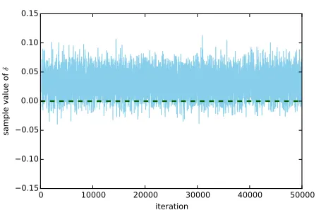
Figure 4: An example trace plot.
We have implemented our models with an MCMC method Metropolis-Hastings sampling [11, 18]. The default configu-ration is to generate 50,000 samples, with no “burn-in”, “lag”, or “multiple-chains”. It has been argued in the MCMC liter-ature that those tricks are often unnecessary: it is perfectly correct to do a single long sampling run and keep all sam-ples [16, 20, 27]. In fact, the approximation accuracy of our program is very high: its Monte Carlo error (MC error) was usually close to 0 and never went beyond 0.002 in all our experiments (see Section 4). Figure 4 shows an exam-ple MCMC trace of our program in the experiments which clearly demonstrates the convergence of MCMC sampling.
In order to calculate the Bayes factor using the SD method (see Section 3.2.1), we approximate the posterior density Pr[δ= 0|M1,D] and the prior density Pr[δ= 0|M1] by fit-ting a smooth function to the corresponding MCMC samples via kernel density estimation (KDE).
The program is written in Python 3 utilising the module
PyMC31 [25] for MCMC based Bayesian model fitting. The source code will be made open to the research community on the first author’s homepage. It is free, easy to use, and extensible to more sophisticated models (see Section 5).
We should mention that this program for Bayesian perfor-mance comparison runs much slower than standard frequen-tist NHST techniques. On a machine with Intel x64 Core i7 CPU 2.30GHz, a sign-test or t-test would normally finish in less than 0.02 seconds, but our program could take up to 20 seconds for one comparison. Most of the time is of course spent on the computationally expensive MCMC sampling. Nevertheless, such a speed should be perfectly acceptable for the purpose of comparing classifiers because the classi-fication experiments would usually take a lot longer time. Therefore the program is still very practical. Moreover, the program could be greatly accelerated by using GPUs via
Theano2, the underlying computational engine forPyMC3.
4.
EXPERIMENTS
4.1
Synthetic Data
To demonstrate the advantage of our paired model over unpaired model, we perform power analysis using
simula-1http://pymc-devs.github.io/pymc3/ 2
http://deeplearning.net/software/theano/
Table 3: The power analysis of our models.
scenario goal dataset-size power
unpaired paired
(a) AB
500 0.26 0.30
1000 0.41 0.52
1500 0.70 0.76
2000 0.79 0.84
2500 0.87 0.90
3000 0.92 0.94
3500 0.96 0.97
(b) A≈B
500 0.00 0.00
1000 0.01 0.22
1500 0.26 0.58
2000 0.63 0.81
2500 0.72 0.87
3000 0.88 0.96
3500 0.92 0.99
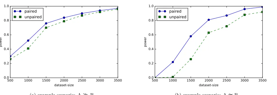
tions. The statistical power is the probability of achieving the goal of a planned empirical study, if a suspected under-lying state of the world is true [18]. As the power increases, there are decreasing chances of a Type II error aka the false negative rateβsince the power is equal to 1−β.
We consider the following two scenarios where the two hypothetical classifiers A and B are somewhat correlated. The scenario (a):
Pr[+] =µ = 0.5
Pr[(1,1)|+] =θ+(1,1)= 0.3, Pr[(1,0)|+] =θ(1,0)+ = 0.3, Pr[(0,1)|+] =θ+
(0,1)= 0.2, Pr[(0,0)|+] =θ +
(0,0)= 0.2, Pr[−] = 1−µ= 0.5
Pr[(1,1)|−] =θ−(1,1)= 0.2, Pr[(1,0)|−] =θ(1,0)− = 0.2, Pr[(0,1)|−] =θ−(0,1)= 0.3, Pr[(0,0)|−] =θ(0,0)− = 0.3, It is easy to see thatF1A= 0.6 whileF1B= 0.5, so the goal here is to detect “AB”.
The scenario (b):
Pr[+] =µ = 0.5
Pr[(1,1)|+] =θ+(1,1)= 0.3, Pr[(1,0)|+] =θ(1,0)+ = 0.2, Pr[(0,1)|+] =θ+
(0,1)= 0.2, Pr[(0,0)|+] =θ +
(0,0)= 0.3, Pr[−] = 1−µ= 0.5
Pr[(1,1)|−] =θ−(1,1)= 0.3, Pr[(1,0)|−] =θ(1,0)− = 0.2, Pr[(0,1)|−] =θ−(0,1)= 0.2, Pr[(0,0)|−] =θ(0,0)− = 0.3, It is easy to see thatF1A= 0.5 andF1B= 0.5, so the goal here is to detect “A≈B”. Please note that this goal is infeasible using the frequentist NHST.
The power analysis results are shown in Table 3 and also Figure 5, which clearly indicate the superiority of our paired model to unpaired model in terms of statistical power.
4.2
Real-World Data
We have conducted our experiments on a standard bench-mark dataset for text classification, 20newsgroups3. In or-der to ensure the reproducibility of our experimental results, we choose to use not the raw document collection, but a publicly-available ready-made “vectorised” version4. It has been split into training (60%) and test (40%) subsets by
3
[image:7.612.330.543.74.255.2]500 1000 1500 2000 2500 3000 3500 dataset-size
0.0 0.2 0.4 0.6 0.8 1.0
power
paired
unpaired
(a) example scenario: AB.
500 1000 1500 2000 2500 3000 3500 dataset-size
0.0 0.2 0.4 0.6 0.8 1.0
power
paired
unpaired
[image:8.612.73.550.59.223.2](b) example scenario: A≈B.
Figure 5: Comparing the statistical power of paired and unpaired models.
date rather than randomly. Following the recommendation of the provider, this dataset has also been “filtered” by strip-ing newsgroup-related metadata (includstrip-ing headers, footers, and quotes). Therefore our reportedF1scores will look sub-stantially lower than those in the related literature, but such an experimental setting is much more realistic and meaning-ful. The same dataset and experimental setting have been used by previous studies on this topic [36].
In the experiments, we have applied our proposed ap-proach to carefully analyse the performances of two well-known supervised machine learning algorithms that are widely used for real-world text classification tasks: Naive Bayes (NB) and linear Support Vector Machine (SVM) [21]. For the former, we consider its two common variations: one with the Bernoulli event model (NBBern) and the other with the Multinomial event model (NBM ult) [22, 23]. For the lat-ter, we consider its two common variations: one with the
L1 penalty (SVML1) and the other with the L2 penalty (SVML2) [10, 37]. Thus we have four different classifiers in total. Obviously, the classification results of NBBernand NBM ultwould be highly correlated, and those of SVML1and SVML2as well. Among them, SVML2is widely regarded as the state-of-the-art text classifier [19,30,34]. It is also worth to notice that the NB algorithms will be applied not to the raw bag-of-words text datasets as people usually do, but on the vectorised20newsgroupsdataset which has already been transformed by TF-IDF term weighting and document length normalisation.
We have used the off-the-shelf implementation of these classification algorithms provided by a Python machine learn-ing libraryscikit-learn5 in our experiments, again for the reproducibility reasons. The smoothing parameterαfor the NB algorithm and the regularisation parameter C for the linear SVM algorithm have been tuned via grid search with 5-fold cross-validation on the training data for the macro-averagedF1score. The optimal parameters found are: NBBern with α = 10−14, NBM ult with α = 10−3, SVML1 with
C= 22, SVML2 withC= 21.
Table 4 shows the results of performance comparison be-tween NBBern and NBM ult, based on which we can confi-dently say that for most of the target categories, NBBern is
5
http://scikit-learn.org/stable/
outperformed by NBM ult. Such results confirm the finding of [22] on this harder dataset.
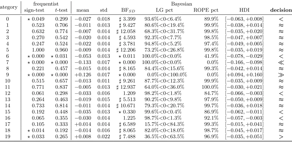
Table 5 shows the results of performance comparison be-tween SVML1 and SVML2, based on which we can confi-dently say that for most of the target categories, SVML1 and SVML2 have no practical difference on classification ef-fectiveness as measured by the F1 score (given the ROPE [−0.05,+0.05]), though the former may have its advantages in terms of sparsity. Such results are complementary to those reported in [37].
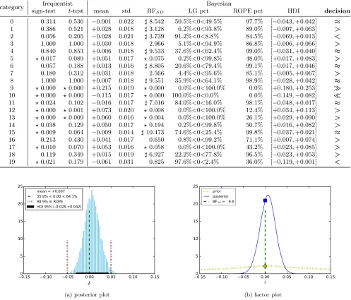
Table 6 shows the results of performance comparison be-tween NBM ultand SVML2 — the better performing classi-fiers from the NB and SVM camps. It can be clearly seen that for most of the target categories, the competition be-tween NBM ult and SVML2 is too close to call: more test data would be needed to make a reliable judgement which one works better. Nevertheless, for six out of eight target categories that we can indeed make a reliable judgement, NBM ult and SVML2 are practically equivalent (given the ROPE [−0.05,+0.05]). This phenomenon somewhat sup-ports the claim of [26] that NBM ult, if properly enhanced by TF-IDF term weighting and document length normalisa-tion, can reach a comparable performance as SVML2.
Since on the micro (document) level, there is not any NHST method existing for the comparison ofF1 scores, we show the results of comparing classification accuracies in those tables: the column “sign-test” contains the two-sided
p-values of using sign-test on the micro level (called s-test in [34]); the column “t-test” contains the two-sidedp-values of using unpaired t-test on the micro level (called p-test in [34]). The symbol ?indicates that the accuracy differ-ence between A and B is statistically significant according to NHST at the levelp <0.05.
Table 4: The results of performance comparison between NBBern and NBM ult.
category frequentist Bayesian
sign-test t-test mean std BFSD LG pct ROPE pct HDI decision
0 ?0.000 ?0.008 −0.081 0.021 ?0.003 100.0%<0<0.0% 6.6% [−0.125,−0.041] <
1 ?0.000 ?0.000 −0.114 0.017 ?0.000 100.0%<0<0.0% 0.0% [−0.148,−0.080]
2 ?0.000 ?0.000 −0.400 0.028 ?0.000 100.0%<0<0.0% 0.0% [−0.456,−0.345]
3 ?0.000 ?0.003 −0.095 0.016 ?0.000 100.0%<0<0.0% 0.2% [−0.126,−0.062]
4 ?0.000 ?0.000 −0.249 0.019 ?0.000 100.0%<0<0.0% 0.0% [−0.286,−0.211]
5 ?0.000 ?0.000 −0.101 0.017 ?0.000 100.0%<0<0.0% 0.1% [−0.135,−0.069]
6 ?0.000 ?0.000 −0.136 0.016 ?0.000 100.0%<0<0.0% 0.0% [−0.168,−0.105]
7 ?0.000 ?0.001 −0.092 0.016 ?0.000 100.0%<0<0.0% 0.4% [−0.123,−0.061]
8 ?0.000 ?0.000 −0.144 0.017 ?0.000 100.0%<0<0.0% 0.0% [−0.178,−0.111]
9 ?0.000 ?0.001 −0.080 0.013 ?0.000 100.0%<0<0.0% 0.8% [−0.105,−0.055]
10 ?0.000 ?0.000 +0.108 0.017 ?0.000 0.0%<0<100.0% 0.0% [+0.074,+0.142]
11 ?0.000 ?0.002 −0.092 0.016 ?0.000 100.0%<0<0.0% 0.4% [−0.125,−0.061]
12 ?0.000 ?0.002 −0.097 0.020 ?0.000 100.0%<0<0.0% 0.8% [−0.137,−0.058]
13 ?0.000 ?0.000 −0.115 0.016 ?0.000 100.0%<0<0.0% 0.0% [−0.147,−0.084]
14 ?0.000 ?0.000 −0.109 0.016 ?0.000 100.0%<0<0.0% 0.0% [−0.139,−0.079]
15 0.064 0.178 −0.027 0.016 ]3.132 95.7%<0<4.3% 92.2% [−0.059,+0.004] <
16 ?0.024 0.151 −0.105 0.019 ?0.000 100.0%<0<0.0% 0.1% [−0.141,−0.068]
17 ?0.000 ?0.000 −0.102 0.016 ?0.000 100.0%<0<0.0% 0.1% [−0.134,−0.070]
18 ?0.000 ?0.034 −0.088 0.020 ?0.007 100.0%<0<0.0% 2.9% [−0.128,−0.049] <
[image:9.612.61.553.347.587.2]19 ?0.000 ?0.011 −0.040 0.030 2.389 91.3%<0<8.7% 62.9% [−0.097,+0.022] <
Table 5: The results of performance comparison between SVML1and SVML2.
category frequentist Bayesian
sign-test t-test mean std BFSD LG pct ROPE pct HDI decision
0 ?0.049 0.299 −0.027 0.018 ]3.399 93.6%<0<6.4% 89.9% [−0.063,+0.008] <
1 0.523 0.706 −0.011 0.013 ]9.427 80.6%<0<19.4% 99.9% [−0.038,+0.014] ≈
2 0.632 0.774 −0.007 0.014 ]12.058 68.3%<0<31.7% 99.8% [−0.035,+0.020] ≈
3 0.270 0.542 −0.020 0.014 ]4.593 92.3%<0<7.7% 98.5% [−0.047,+0.007] ≈
4 0.247 0.524 −0.022 0.014 ]3.781 94.8%<0<5.2% 97.4% [−0.049,+0.005] ≈
5 1.000 0.960 −0.009 0.014 ]12.206 73.2%<0<26.8% 99.8% [−0.035,+0.019] ≈
6 ?0.000 ?0.031 −0.053 0.013 ?0.011 100.0%<0<0.0% 41.9% [−0.078,−0.029] <
7 ?0.000 ?0.000 −0.133 0.017 ?0.000 100.0%<0<0.0% 0.0% [−0.166,−0.098]
8 0.221 0.457 −0.015 0.014 ]8.165 84.4%<0<15.6% 99.3% [−0.042,+0.014] ≈
9 ?0.000 ?0.000 +0.126 0.017 ?0.000 0.0%<0<100.0% 0.0% [+0.094,+0.160]
10 0.515 0.657 −0.013 0.011 ]9.261 87.7%<0<12.3% 99.9% [−0.035,+0.009] ≈
11 0.771 0.837 −0.005 0.013 ]12.937 64.0%<0<36.0% 100.0% [−0.030,+0.021] ≈
12 0.061 0.298 −0.033 0.016 1.209 98.2%<0<1.8% 84.7% [−0.066,−0.003] <
13 0.264 0.463 −0.019 0.015 ]5.513 90.2%<0<9.8% 97.9% [−0.050,+0.009] ≈
14 0.733 0.814 −0.011 0.014 ]10.671 79.3%<0<20.7% 99.7% [−0.036,+0.018] ≈
15 0.192 0.448 −0.035 0.013 ?0.330 99.6%<0<0.4% 86.9% [−0.062,−0.011] <
16 0.065 0.355 −0.030 0.014 1.225 98.7%<0<1.3% 92.1% [−0.057,−0.003] <
17 0.105 0.333 +0.014 0.014 ]6.589 15.7%<0<84.3% 99.3% [−0.015,+0.041] ≈
18 ?0.014 0.192 −0.014 0.016 ]8.065 82.0%<0<18.0% 98.7% [−0.045,+0.017] ≈
19 ?0.033 0.265 +0.008 0.022 ]7.488 36.5%<0<63.5% 96.9% [−0.035,+0.051] >
approach has only thep-values (and maybe also the confi-dence intervals) to offer. Furthermore, note that the judge-ments made by the Bayesian estimation on several cases are different from those made by the frequentist NHST (e.g., at the significance level 0.05). So even if in some researchers’ opinion the superiority of the former over the latter is still debatable, there is no doubt that the former can at least be complementary to the latter.
Figure 6 illustrates the visualisation of Bayesian perfor-mance comparison results produced by our program: the
“posterior plot” sub-graph shows the posterior probability distribution of the performance difference variable δ; and the “factor plot” sub-graph shows the estimation of the Bayes factor by the SD method.
5.
EXTENSIONS
Table 6: The results of performance comparison between NBM ult and SVML2.
category frequentist Bayesian
sign-test t-test mean std BFSD LG pct ROPE pct HDI decision
0 0.314 0.536 −0.001 0.022 ]8.542 50.5%<0<49.5% 97.7% [−0.043,+0.042] ≈
1 0.386 0.521 +0.028 0.018 ]3.128 6.2%<0<93.8% 89.0% [−0.007,+0.063] >
2 0.056 0.205 −0.028 0.021 ]3.739 91.2%<0<8.8% 84.5% [−0.069,+0.013] <
3 1.000 1.000 +0.030 0.018 2.966 5.1%<0<94.9% 86.8% [−0.006,+0.066] >
4 0.840 0.853 +0.006 0.018 ]9.533 37.6%<0<62.4% 99.0% [−0.031,+0.040] ≈
5 ?0.017 0.089 +0.051 0.017 ?0.075 0.2%<0<99.8% 48.0% [+0.017,+0.083] >
6 0.057 0.188 +0.013 0.016 ]8.805 20.6%<0<79.4% 99.1% [−0.017,+0.046] ≈
7 0.180 0.312 +0.031 0.018 2.566 4.4%<0<95.6% 85.1% [−0.005,+0.067] >
8 1.000 1.000 +0.007 0.018 ]9.551 35.9%<0<64.1% 98.9% [−0.028,+0.042] ≈
9 ?0.000 ?0.000 +0.215 0.019 ?0.000 0.0%<0<100.0% 0.0% [+0.180,+0.253]
10 ?0.000 ?0.000 −0.115 0.017 ?0.000 100.0%<0<0.0% 0.0% [−0.149,−0.082]
11 ?0.024 0.102 −0.016 0.017 ]7.016 84.0%<0<16.0% 98.1% [−0.048,+0.017] ≈
12 ?0.000 ?0.001 +0.073 0.020 ?0.008 0.0%<0<100.0% 12.4% [+0.034,+0.113] >
13 ?0.000 ?0.009 +0.060 0.016 ?0.004 0.0%<0<100.0% 26.1% [+0.029,+0.090] >
14 ?0.038 0.129 +0.050 0.017 ?0.194 0.2%<0<99.8% 50.7% [+0.016,+0.082] >
15 ?0.009 0.064 −0.009 0.014 ]10.473 74.6%<0<25.4% 99.8% [−0.037,+0.021] ≈
16 0.213 0.430 +0.041 0.017 0.650 0.8%<0<99.2% 71.1% [+0.007,+0.074] >
17 ?0.010 0.070 +0.053 0.016 ?0.058 0.0%<0<100.0% 43.2% [+0.023,+0.085] >
18 0.119 0.349 +0.015 0.019 ]6.927 22.2%<0<77.8% 96.5% [−0.023,+0.053] >
19 ?0.021 0.179 −0.061 0.031 0.825 97.6%<0<2.4% 36.0% [−0.119,+0.001] <
0.15 0.10 0.05 0.00 0.05 0.10 0.15
δ
0 5 10 15 20 25
mean = +0.007 35.9% < 0.00 < 64.1% 98.9% in ROPE HDI 95% [-0.028,+0.042]
(a) posterior plot
0.15 0.10 0.05 0.00 0.05 0.10 0.15 δ
0 5 10 15 20 25
prior posterior
BFSD = 9.6
(b) factor plot
Figure 6: A≈B — NBM ultis practically equivalent to SVML2for target category 8.
Multiple classes. It would be straightforward to extend our model to multi-class classification (either single-label or multi-label): we will need one µ parameter and a pair of
θparameters for each class. Thus we are able to measure each classifier’s overall performance using micro-averaged or macro-averagedF1scores [34], and compute their difference as the deterministic variableδ in the model [35]. Note that hereδ is estimated using a large number of prediction out-comes for all test documents, rather than just a small num-ber ofF1scores for test categories as in [34] (see Section 2.1). It would be promising to go further to develop a Bayesian hi-erarchical model [11, 18] where the classifier’s parametersθj for different classes are governed by a higher-level overarch-ing hyper-parameterη(e.g., representing the overall proba-bility of making correct predictions) and thus able to “share statistical strength” [36]. A potential problem, though, is the explosive growth of possible prediction outcome
combi-nations along with the increase of class numbers, which in the worst situation may force us into backing off to the as-sumption of independence between classifiers so as to keep the model computationally tractable.
Other performance measures. To compare classifiers using a performance measure different from the F1 score, we would only need to replace the functionf(µ,θ+,θ−) for computingψ, as long as that performance measure could be calculated based on the classification contingency table alone [15]. For example, it would be straightforward to extend our probabilistic model to handle the more generalFβ measure (β ≥ 0) with β 6= 1 [21, 31]. Since the Area Under the ROC Curve (AUC) is essentially the proportion of correctly ranked document pairs [15], it could be modelled in a similar way.
[image:10.612.57.554.77.502.2]comprehen-sive performance comparison could be applied to not just classifiers, but also search systems (see the ICTIR-2015 best paper [4]), recommender systems, and advertising systems.
6.
CONCLUSIONS
In this paper, we have tried to address the problem of com-paring text classifiers’ performances by appealing to Bayesian reasoning. Although we ourselves believe that Bayesian statis-tics is “the way it should be”, we understand that not ev-eryone is a Bayesian or wants to become a Bayesian. Our argument is not whether being a Bayesian is philosophically better than being a frequentist, but that our Bayesian esti-mation based approach to performance comparison of text classifiers avoids a number of practical weaknesses of NHST and it provides much richer information about the differ-ence between two classifiers’ performances than NHST does, therefore it can supersede the currently popular frequentist approach.
7.
[1] D. Barber. Are two classifiers performing equally? a treatmentREFERENCES
using Bayesian hypothesis testing. Technical report, IDIAP, 2004.
[2] D. Barber.Bayesian Reasoning and Machine Learning.
Cambridge University Press, 2012.
[3] A. Blum and T. Mitchell. Combining labeled and unlabeled
data with co-training. InProceedings of the 11th Annual
Conference on Computational Learning Theory (COLT), pages 92–100, Madison, WI, 1998.
[4] B. Carterette. Bayesian inference for information retrieval
evaluation. InProceedings of the 2015 International
Conference on the Theory of Information Retrieval (ICTIR), pages 31–40, Northampton, MA, USA, 2015.
[5] K. W. Church and P. Hanks. Word association norms, mutual
information, and lexicography.Computational Linguistics,
16(1):22–29, 1990.
[6] J. Demˇsar. Statistical comparisons of classifiers over multiple
data sets.The Journal of Machine Learning Research
(JMLR), 7:1–30, 2006.
[7] J. M. Dickey and B. P. Lientz. The weighted likelihood ratio, sharp hypotheses about chances, the order of a markov chain. The Annals of Mathematical Statistics, 41(1):214–226, 1970. [8] Z. Dienes. Bayesian versus orthodox statistics: Which side are
you on?Perspectives on Psychological Science, 6(3):274–290,
2011.
[9] T. G. Dietterich. Approximate statistical tests for comparing
supervised classification learning algorithms.Neural
Computation, 10(7):1895–1923, 1998.
[10] R.-E. Fan, K.-W. Chang, C.-J. Hsieh, X.-R. Wang, and C.-J. Lin. LIBLINEAR: A library for large linear classification. Journal of Machine Learning Research, 9:1871–1874, 2008. [11] A. Gelman, J. Carlin, H. Stern, D. Dunson, A. Vehtari, and
D. Rubin.Bayesian Data Analysis. Chapman & Hall/CRC,
3rd edition, 2013.
[12] C. Goutte and E. Gaussier. A probabilistic interpretation of
precision, recall andF-score, with implication for evaluation. In
Proceedings of the 27th European Conference on IR Research (ECIR), pages 345–359, Santiago de Compostela, Spain, 2005.
[13] T. Hastie, R. Tibshirani, and J. Friedman.The Elements of
Statistical Learning: Data Mining, Inference, and Prediction. Springer, 2nd edition, 2009.
[14] D. A. Hull. Improving text retrieval for the routing problem
using latent semantic indexing. InProceedings of the 17th
Annual International ACM SIGIR Conference on Research and Development in Information Retrieval (SIGIR), pages 282–291, Dublin, Ireland, 1994.
[15] T. Joachims. A support vector method for multivariate
performance measures. InProceedings of the 22nd
International Conference on Machine Learning (ICML), pages 377–384, Bonn, Germany, 2005.
[16] D. Koller and N. Friedman.Probabilistic Graphical Models
-Principles and Techniques. MIT Press, 2009.
[17] J. K. Kruschke. Bayesian estimation supersedes the t test. Journal of Experimental Psychology: General, 142(2):573, 2013.
[18] J. K. Kruschke.Doing Bayesian Data Analysis: A Tutorial
with R, JAGS, and Stan. Academic Press, 2nd edition, 2014. [19] D. D. Lewis, Y. Yang, T. G. Rose, and F. Li. RCV1: A new
benchmark collection for text categorization research.Journal
of Machine Learning Research (JMLR), 5:361–397, 2004.
[20] D. J. C. MacKay.Information Theory, Inference, and
Learning Algorithms. Cambridge University Press, 2003.
[21] C. D. Manning, P. Raghavan, and H. Sch¨utze.Introduction to
Information Retrieval. Cambridge University Press, 2008. [22] A. McCallum and K. Nigam. A comparison of event models for
Naive Bayes text classification. InAAAI-98 Workshop on
Learning for Text Categorization, pages 41–48, Madison, WI, 1998.
[23] V. Metsis, I. Androutsopoulos, and G. Paliouras. Spam filtering
with Naive Bayes - which Naive Bayes? InProceedings of the
3rd Conference on Email and Anti-Spam (CEAS), pages 27–28, Mountain View, CA, USA, 2006.
[24] T. Mitchell.Machine Learning. McGraw Hill, 1997.
[25] A. Patil, D. Huard, and C. J. Fonnesbeck. PyMC: Bayesian
stochastic modelling in Python.Journal of Statistical
Software, 35(4):1–81, 2010.
[26] J. D. Rennie, L. Shih, J. Teevan, and D. R. Karger. Tackling the poor assumptions of Naive Bayes text classifiers. In Proceedings of the 20th International Conference on Machine Learning (ICML), pages 616–623, Washington, DC, USA, 2003. [27] P. Resnik and E. Hardisty. Gibbs sampling for the uninitiated.
Technical Report LAMP-TR-153, Defense Technical Information Center (DTIC), 2010.
[28] J. N. Rouder, P. L. Speckman, D. Sun, R. D. Morey, and
G. Iverson. Bayesianttests for accepting and rejecting the null
hypothesis.Psychonomic Bulletin & Review, 16(2):225–237,
2009.
[29] H. Schutze, D. A. Hull, and J. O. Pedersen. A comparison of classifiers and document representations for the routing
problem. InProceedings of the 18th Annual International
ACM SIGIR Conference on Research and Development in Information Retrieval (SIGIR), pages 229–237, Seattle, WA, USA, 1995.
[30] F. Sebastiani. Machine learning in automated text
categorization.ACM Computing Surveys (CSUR), 34(1):1–47,
2002.
[31] C. J. van Rijsbergen.Information Retrieval. Butterworths,
London, UK, 2nd edition, 1979.
[32] E.-J. Wagenmakers, T. Lodewyckx, H. Kuriyal, and
R. Grasman. Bayesian hypothesis testing for psychologists: A
tutorial on the Savage-Dickey method.Cognitive Psychology,
60(3):158–189, 2010.
[33] R. Wetzels, J. G. Raaijmakers, E. Jakab, and E.-J.
Wagenmakers. How to quantify support for and against the null hypothesis: A flexible WinBUGS implementation of a default
Bayesianttest.Psychonomic Bulletin & Review,
16(4):752–760, 2009.
[34] Y. Yang and X. Liu. A re-examination of text categorization
methods. InProceedings of the 22nd Annual International
ACM SIGIR Conference on Research and Development in Information Retrieval (SIGIR), pages 42–49, Berkeley, CA, USA, 1999.
[35] D. Zhang, J. Wang, and X. Zhao. Estimating the uncertainty of
average F1 scores. InProceedings of the 2015 International
Conference on the Theory of Information Retrieval (ICTIR), pages 317–320, Northampton, MA, USA, 2015.
[36] D. Zhang, J. Wang, X. Zhao, and X. Wang. A bayesian hierarchical model for comparing average F1 scores. In Proceedings of the 2015 IEEE International Conference on Data Mining (ICDM), pages 589–598, Atlantic City, NJ, USA, 2015.
[37] J. Zhu, S. Rosset, T. Hastie, and R. Tibshirani. 1-norm support
vector machines. InAdvances in Neural Information