Motion Anisotropy Analysis of the Four Wheeled Mobile Robot

2017 2nd International Conference on Computer, Mechatronics and Electronic Engineering (CMEE 2017) ISBN: 978-1-60595-532-2

Motion Anisotropy Analysis of the Four Wheeled Mobile Robot

Wei-hua ZHOU and De-fa ZHANG

Taizhou Vocational & Technical College, Taizhou, Zhejiang 318000

Keywords: Mobile robot, Kinematic, Dynamics, Anisotropy.

Abstract. The anisotropy of velocity and acceleration was analyzed in this paper based on the four wheeled mobile robot which composed of single row alternate wheels.Firstly, the kinematics equation of the mobile robot was derived, and the maximum velocity values in different directions were calculated. The simulation result was identical with the theoretical values by ADAMS software. Then, the dynamic equation of the mobile robot was established according to the Routh equation of nonlinear system. Finally, the acceleration value of the mobile robot was acquired by theelectrical sensor. The experimental result was in agreement with the theoretical values.

Introduction

Considering the special structure of the single row alternate wheel, the kinematics and dynamic characteristics of the mobile robot are different withthe two wheeled robot and the crawler robot.

Many experts and scholars have studied the motion anisotropy of mobile robot at home and abroad. Wade [1, 2] proposed the stepless-speed regulation of mobile robot by changing the structure of the wheels. However, it’s difficult to change thestructure, and the bearing capacity of the structure is limited. Ashmore [3] presented that the maximum speed of a mobile robot changes with the number of wheels. According to LengChuntao’s analysis [4], the maximum speed and maximum acceleration are different in different directions. And the geometric relationship between the center of the robot and the wheelwas established.

The kinematic and dynamic characteristics of four wheeled mobile robots which based on single rowalternate wheels were analyzed in this paper. The speed anisotropy of the mobile robot was verified by ADAMS software simulation, and the acceleration anisotropy was verified by experiments.

Structure of the Mobile Robot

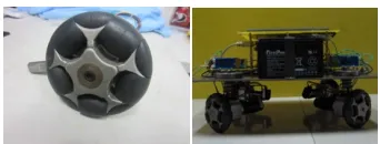
Figure 1. Alternate wheel and four wheeled mobile robot.

The alternate wheel was made by nesting rollers, as shown in figure 1. The section of the nesting rollersare on the same circumference, so that the contact height between the wheel and the ground isn’tchanged when the wheel is rolling.The rolling bearings were installed at the middle of the hub [5]

.

Anisotropy Analysis of Kinamics W1 W2 W3 W4 O XM YM V a

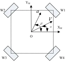
Figure 2. Motion diagrammatic sketch.

The four wheelswereorthogonal and symmetrically arranged. The inverse kinematics equation of the mobile robot can be obtained:

          ⋅ =               ω ω ω ω ω y x V V R 4 3 2 1 ,               − − − − ⋅ = l l l l r 2 1 1 2 1 1 2 1 1 2 1 1 2 2

R (1)

ω1~ω4 denote the rotationangular velocity of the four wheels, Vx, Vy, ω denote the XM axis speed, YM axis speed and rotation angular velocity around the center axis of the mobile robot respectively.

R is the inverse kinematics matrix. Thus,               ⋅                   − − − − =           4 3 2 1 4 4 4 4 4 2 4 2 4 2 4 2 4 2 4 2 4 2 4 2 ω ω ω ω ω l r l r l r l r r r r r r r r r V V y x (2)

Assume that the angle between the velocity and the robot coordinate system is α, as shown in Figure 2. The value of velocity can be obtained:

α

α

cos V V

V

V_x = ， _y = (3)

) 2 2 ( 4 1 4 2 3 1 2 4 2 3 2 2 2 1 2 2

2 _{ϕ ϕ ϕ ϕ ϕϕ ϕϕ}

+ + + − − = +

= V V r

V _{x y} (4)

The motion of the wheel is generated by the motor. Considering the limitation of theactualmotor speed, the speed range of the four wheels is:

4 ~ 1 i (rad/s), 49 . 10 (rad/s) 49 .

10 ≤ i ≤ ∈

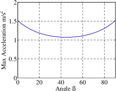
Figure 3. The maximum of V in all directions.

According to the result of Figure 3, the amplitude of velocity is the maximumwhen the angle between velocity and XM is 90°.The amplitude of the velocity is minimumwhen the angle between the velocity and the XM is 45°.

In order to verify the speed anisotropy of mobile robot, the ADAMS software was used to verify the theoretical calculation value, and the simulation model was set up as shown in the Figure 4.

Figure 4. Simulation model of the mobile robot.

In the ADAMS software, the related construction and synthesis are integrated by Boolean operation, such as the integration of the hub and roller shaft, the integration of the bracket and wheel hub.Define kinematic pair as:

(1) Rotary motion pair between wheels and connecting shafts. (2) Rotary motion pair between roller and roller shaft.

The simulation result is shown in Figure 5.

Figure 5. Simulation results of velocity in all directions.

0 20 40 60 80

0 0.2 0.4 0.6 0.8

Angle α

Ma

x

V

el

o

ci

ty

m/

s

0 20 40 60 80

0 0.2 0.4 0.6 0.8

Angle α

M

ax

V

el

o

ci

ty

m

The simulation results are in good agreement with the theoretical values, which shows that the velocity anisotropy of the mobile robot calculated is completely correctby this method.

AnisotropyAnalysis of Dynamics

The acceleration of the mobile robot is related to the dynamics of wheel. Lagrange method [8], Newton-Euler method [9], Gauss method [10] are widely used to solve the wheel dynamic problem without slippage. The Lagrange method can be solved by using the speed of each part. The method is relatively simple. Therefore, the Lagrange method of nonholonomic system -- also called the Routh methodis used to solve the dynamics of mobile robot in this paper [11].

The acceleration of the mobile robot and the wheel is calculated from formula (2).

              ⋅               =           ⋅                       − − − − 4 3 2 1 0 0 0 0 0 0 0 0 0 0 0 0 2 2 2 2 2 2 2 2 2 2 2 2 2 2 2 2 ω ω ω ω ω r r r r V V l l l l y x (6)

The mobile robot system is the nonholonomic constraint system. The speed Vx, Vy, ω and wheel speed can’t be decoupled. According to the Routh equation [7] of the nonholonomic system, the dynamic equation is:

) , 2 , 1 ( 1 l j B Q q T q T dt d s k kj k j j j ⋅ ⋅ ⋅ ⋅ = + = ∂ ∂ − ∂ ∂

∑

qj, Qj denote generalized coordinates and generalized forces, Tdonotes kinetic energy,λk denotes undetermined Lagrange multipliers, Bkj denotes constraint coefficients.

The kinetic energy of the mobile robot includes translational energy, rotational energy and kinetic energy of the four wheels.M denotes the mass of the mobile robot. The kinetic energy of themobile robot can be expressed as [12]:

∑

x MV J J J

MV

T ω ω ω (8) Jω, Jmdonoterotary inertia of the wheel and the roller.

Ta1, Ta2, Ta3, Ta4 denote the effective driving torque of the wheels, thus: ) 4 ~ 1 , 7 ~ 4 ( , = =

=T i j

Qi aj (9) The solution formula (8) can be solved according to the Routh equation:

The undetermined Lagrange multipliercan be obtained: 4 ~ 1 , ) ( = + − = i r J J

T_{ai m i}

i

ω

λ ω

(11) The dynamic equations of the four wheeled mobile robot are solved according to the formula (6), (9), (10) and (11), as follows:

          + + + = + ⋅ + − + + − = + ⋅ + − − + = + ⋅ + ) ( ) ) ( 4 ( ) ( 2 2 ) 2 ( ) ( 2 2 ) 2 ( 4 3 2 1 4 3 2 1 4 3 2 1 0 2 2 2 2 a a a a a a a a a a a a T T T T r l r J J l J T T T T r V r J J M T T T T r V r J J M m y m x m ω ω ω ω (12)

Assume that the direction of the acceleration and the mobile robot coordinate XMis βangle.

β β, sin

cos V a

a

Vx = y= (13)

4 2 3 1 2 4 2 3 2 2 2 1 2 2 2 2 2

2 m a a a a a a a a

y

x T T T T T T T T

J J Mr r V V

a ⋅ + + + − −

+ + = + = ） （ ω (14) The tangential reaction of the wheel to the ground is the cause of the motion. The limit value of the tangential reaction force is called the adhesion force Fh. The magnitude of adhesion force is equal to the product of the positive pressure and adhesion coefficient of the wheelµh. The coefficient of adhesion µh is determined by the material of the ground and the wheel, and the value is 1. Meanwhile, the wheels are affected by the rolling friction between the wheels and the ground.The rolling friction force of each wheel is 0.25Mgµf. In summary, the range of effective output torque of each wheel is:

4 ~ 1 , ) ( 4 1 ) ( 4 1 ∈ − ≤ ≤ −

− Mg µ_h µ_f r T_ai Mg µ_h µ_f r i (15) The value of the formula (14) can be obtained under the constraints of (12), (13) and (15) constraints. The results can be calculated by using the quaprog function in Matlab, as shown in Figure 6.

Figure 6. The theoretical value of acceleration in all directions.

The mobile robot was designed and manufacturedin order to verify the correctness of the theoretical analysis. The industrial control board wasused as the controller of mobile robot. A

0 20 40 60 80

0 0.5 1 1.5 2

Angle β

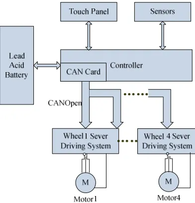
CANOpen communication network was formed by the CAN ports of the motor driversand the industrial control board by extending the CAN card. All data sending and receiving was realized by CANOpen network. The highest communication rate is 1Mbit/s. The block diagram of the control system of the mobile robot is shown in Figure 7.

Figure 7. Block diagram of mobile robot control system.

Acceleration was measured by the sensor MPU6050 which installed in the centre of the mobile robot.Taking into account the symmetry of the mobile robot, the experiment only measured the data of the first quadrant. The experimental results are shown in Figure 8.

Figure 8. Experimental results of acceleration in all directions.

According to the experimental results of Figure 8, the theoretical value is basically consistent with the actual value.But there are also some deviations, due to the following factors mainly:

(1) Machining deviation of mobile robot. The theoretical value is calculated according to the idealized model. The actual mobile robot has the machining error, bearing friction and other factors. (2) The dynamic friction force is variable in wheel motion, but the value is equivalent to a constant value in the theoretical calculation.

(3) The precision error and installation error of the acceleration sensor.

Conclusion

A practical single row alternate wheel and a mobile robot arepresented in this paper.The following

0 20 40 60 80

0 0.5 1 1.5 2

Angle β

M

ax

A

cc

el

er

at

io

n

m

/s

(1) The velocity anisotropy of the mobile robot obtained by inverse kinematics is the same as that of the ADAMS software.

(2) The maximum acceleration of each direction of the mobile robot is given and verified by experiment.

(3) It can be used as a reference for the path planning and optimal controlling of the mobile robot.

Acknowledgments

This research was financially supported by the Taizhou Science and Technology Plan Project (1701gy25), and Zhejiang Province Education Department Project (Y201636417).

Reference

[1] M Wade, H H Asada. Design and control of a variable footprint mechanism for holonomic omnidirectional vehicles and its application to wheelchairs[C]//IEEE International Conference on Robotics and Automation, Japan, 1999:978-989.

[2] J B Song, K S Byun.Design and Control of a Four-Wheeled Omnidirectional Mobile Robot with Steerable Omnidirectional Wheels[J].Journal of Robotic Systems, 2004, 21(4):193-208.

[3] M Ashmore, N Barnes. Omni-drive robot motionon curved pahts: the fastest path between two points is not a straight-line [C]//Australian Joint Conference on Artifical Intelligence,Canberra, Australia, 2002:225-233.

[4] Wang Ban, Zhou Wei-hua, Guo Ji-feng, et al. Structure and analysis of an omni-directional wheel with circular conical wheel[J]. China Mechanical Engineering, 24(15):2015-2019.

[5] Zhou Wei-hua, Wang Ban, Guo Ji-feng. Self-lock characteristics of alternate wheel and the mobile robot[J]. Robot, 2013, 35(4):449-455.

[6] Zhou Wei-hua, Wang Ban, Huang Shan-jun, et al. Layout selection and stability analysis of a mobile robot based on single row alternate wheel[J]. China Mechanical Engineering, 2014, 25(7):888-894.

[7] Cleve B.Moler. Numerical computing with matlab[M]. Beijing: Beijing Aerospace University Press, 2015.

[8] Wu Ke-he, Li Wei, Liu Chang-an, et al. Dynamic control of two-wheeled mobile robot[J].Journal of Astronautics Astrona, 2006, 27(2):273-275.

[9] Mei Hong, Wang Yong. Dynamic modeling and tracking control for wheeled mobile robot[J]. Machine Tool & Hydraulics, 2009, 37(9):127-129.

[10] Liu Yu, Ren Jun-guo, Tang Qian-gang. Gauss elimination method of flexibility dynamic equation[J]. Journal of Hunan Institute of Science and Technology, 2004, 17(1):16-18.

[11] Liu Yan-zhu. Advanced dynamics[M]. Beijing: Advanced Education Press, 2001.