University of Huddersfield Repository
Azevedo, A., Neves, Sérgio and Calcada, R.Dynamic analysis of the trainbridge interaction: an accurate and efficient numerical method Original Citation
Azevedo, A., Neves, Sérgio and Calcada, R. (2008) Dynamic analysis of the trainbridge interaction: an accurate and efficient numerical method. In: EURODYN 2008 7th European Conference on Structural Dynamics, 7th9th July 2008, Southampton, United Kingdom. This version is available at http://eprints.hud.ac.uk/id/eprint/23130/
The University Repository is a digital collection of the research output of the University, available on Open Access. Copyright and Moral Rights for the items on this site are retained by the individual author and/or other copyright owners. Users may access full items free of charge; copies of full text items generally can be reproduced, displayed or performed and given to third parties in any format or medium for personal research or study, educational or notforprofit purposes without prior permission or charge, provided:
• The authors, title and full bibliographic details is credited in any copy; • A hyperlink and/or URL is included for the original metadata page; and • The content is not changed in any way.
For more information, including our policy and submission procedure, please contact the Repository Team at: [email protected].
DYNAMIC ANALYSIS OF THE TRAIN-BRIDGE INTERACTION: AN
ACCURATE AND EFFICIENT NUMERICAL METHOD
Álvaro Azevedo1, Sérgio Neves2* and Rui Calçada2
1
Department of Civil Engineering Faculty of Engineering
University of Porto
Rua Dr. Roberto Frias, s/n, 4200-465 Porto, Portugal E-mail: [email protected] Web: http://www.fe.up.pt/~alvaro
2
Department of Civil Engineering Faculty of Engineering
University of Porto
Rua Dr. Roberto Frias, s/n, 4200-465 Porto, Portugal E-mail: {sgneves,ruiabc}@fe.up.pt Web: http://www.fe.up.pt
Keywords: Train-bridge interaction, dynamic analysis, HHT method, finite element method.
ABSTRACT
1. INTRODUCTION
The dynamic behavior of railway bridges carrying high-speed trains can be analyzed with or without the consideration of the vehicle's own structure. The simulation of the train-bridge system requires several independent submeshes and the consideration of contact conditions that represent their interaction.
Delgado and Cruz [1] and Calçada [2] developed a computational methodology to analyze the train-bridge interaction. This methodology was implemented in a previous version of FEMIX, which is a general purpose finite element computer program [3]. The developed algorithm is very versatile, allowing the modeling of any structure and vehicle using 3D beam elements. However the treatment of the contact conditions between the independent submeshes is performed by an iterative process, which can be inefficient.
This paper describes the formulation of the contact between nodal points of the vehicle and internal points of a finite element. Dynamic equilibrium equations in non prescribed degrees of freedom, in contact degrees of freedom and in prescribed degrees of freedom are separately developed. Contact compatibility equations between points of the vehicle and internal points of a finite element are also separately developed. All these equations constitute a single system of linear equations involving displacements, contact forces and reactions as unknowns. After the solution of this system of linear equations the displacements, velocities and accelerations at the current time step can be calculated and a new time step is started. This heterogeneous system of linear equations can be efficiently solved by means of the consideration of several submatrices with specific characteristics.
The new formulation described here is applied to the analysis of the dynamic behavior of the São Lourenço bridge, which is a bowstring arch bridge. The bridge is located in the North Line of the Portuguese railway system, in a section that was recently upgraded to allow the passage of the Alfa pendular train at greater speeds. The numerical model was validated with the results of the ambient vibration test and those measured during several passages of the Alfa pendular train. The dynamic response of the train-bridge system was calculated for train speeds exceeding the allowable speed for that section of the North Line.
2. HHT METHOD WITH TRAIN-BRIDGE INTERACTION
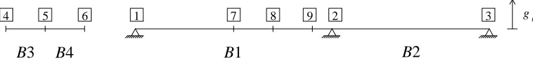
A simple example is used to introduce the types of degrees of freedom that are considered in the formulation of the vehicle-structure interaction in the context of a time step of the Hilber-Hughes-Taylor method (see Figure 1). On the right, a simply supported beam with two spans (B1 and B2) is subjected to the contact of a vehicle, shown on the left. The structure of the vehicle is also composed of two beams (B3 and B4). Nodes 7, 8 and 9 are internal points of the beam B1. The location of these nodes may change between time steps, depending on the position of the vehicle. Eventual gaps between both structures (gi) can be easily considered in
[image:3.595.100.487.668.714.2]the compatibility equations, as will be shown later.
Figure 1. Vehicle and structure: beams and nodal points
1 7 8 9 2 3
6 5 4
B3
gi
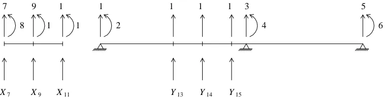
In each nodal point two degrees of freedom are considered (vertical displacement and rotation). Figure 2 shows the generalized displacements in nodal points (1 to 12), the generalized displacements of the contact points of the structure (13, 14 and 15), the interaction forces in the vehicle (X7, X9 and X11) and the interaction forces in the structure (Y13, Y14 and
[image:4.595.109.488.167.266.2]Y15). The interaction only involves the translational degrees of freedom.
Figure 2. Vehicle and structure: degrees of freedom and interactions forces
The following classification of the degrees of freedom is considered:
• F – free;
• X – interaction (vehicle);
• P – prescribed;
• Y – interaction (structure).
This classification is used later in this section.
In the context of the Hilber-Hughes-Taylor method (HHT), the dynamic equilibrium equation that involves the degrees of freedom in nodal points (1 to 12) is the following
(
)
c p(
)
c p(
)
c pc
α α
α α
α
α Cu Cu Ku Ku F F
u
Mɺɺ + 1+ ɺ − ɺ + 1+ − = 1+ − (1)
In this equation M is the mass matrix, C is the damping matrix, K is the stiffness matrix, F
are the applied generalized forces, u are the generalized displacements and
α
is the main parameter of the HHT method. Whenα
= 0 the HHT method reduces to the Newmark method, and for other values of the parameterα
, numerical energy dissipation is introduced in the higher modes. The superscript c indicates the current time step (t + ∆t) and the superscriptp indicates the previous one (t).
According to Figure 2 and to the classification indicated above, the F type degrees of
freedom are the following: 2, 4, 6, 8, 10 and 12. The X type degrees of freedom correspond to
the "supports" of the separated vehicle structure, being the following: 7, 9 and 11. The P type
degrees of freedom are the main structural supports 1, 3 and 5. The Y type degrees of freedom
13, 14 and 15 consist on the internal displacements of beam B1 at the contact points.
According to this classification of degrees of freedom, Eq. (1) can be expanded by considering several submatrices, yielding
7 8
9 1
1 1
1 2
3 4
5 6
1 1 1
Y 13 Y 14 Y 15
X 11
X 9
(
)
(
)
(
)
+ + + + − + + + + + = − + + − + + p P p Y PY p P p X XX p X p Y FY p F c P c Y PY c P c X XX c X c Y FY c F p P p X p F PP PX PF XP XX XF FP FX FF c P c X c F PP PX PF XP XX XF FP FX FF p P p X p F PP PX PF XP XX XF FP FX FF c P c X c F PP PX PF XP XX XF FP FX FF c P c X c F PP PX PF XP XX XF FP FX FF α α α α α α R Y d P X I P Y d P R Y d P X I P Y d P u u u K K K K K K K K K u u u K K K K K K K K K u u u C C C C C C C C C u u u C C C C C C C C C u u u M M M M M M M M M 1 1 1 ɺ ɺ ɺ ɺ ɺ ɺ ɺ ɺ ɺ ɺ ɺ ɺ (2)In the F type degrees of freedom,
Y FY F
F P d Y
F = + (3)
being P the external loads applied in correspondence with each degree of freedom. Each component dij of dFY corresponds to the nodal force in the F type degree of freedom i, which is
equivalent to a single load consisting of a unitary value of Yj (see Figure 2).
In the X type degrees of freedom,
X XX X
X P I X
F = + (4)
being IXX the identity matrix with an appropriate size.
In the P type degrees of freedom,
P Y PY P
P P d Y R
F = + + (5)
being RP the reactions.
According to Figure 2, equilibrium equations in the contact degrees of freedom can be written, yielding
X Y X
Y =− (6)
Since the number of Y type degrees of freedom coincides with the number of X type degrees of freedom, the subscript Y may be replaced with X.
According to [4], Eq. (2) is equivalent to the following three equations
(
)
Fc X FX c X FX c F
FFu K u α d X F
(
)
X c X XX c X XX c FXFu K u α I X F
K + − 1+ = (8)
p P PP p X PX p F PF c P PP c X PX c F PF p P PP p X PX p F PF c P PP c X PX c F PF c P PP c X PX c F PF p X PX c X PX p P c P p P c P α α α α α α α α α α α α α α α α α α α α α u K u K u K u K u K u K u C u C u C u C u C u C u M u M u M X d X d P P R R + − + − + − + + + + − + − + − + + + + + + + + + + − + + + − + = 1 1 1 1 1 1 1 1 1 1 1 1 1 1 1 ɺ ɺ ɺ ɺ ɺ ɺ ɺ ɺ ɺ ɺ ɺ ɺ (9) being
(
)
FF(
)
FFFF
FF A M α AC α K
K = 0 + 1+ 1 + 1+ (10)
(
)
FX(
)
FXFX
FX A M α AC α K
K = 0 + 1+ 1 + 1+
(
)
XF(
)
XFXF
XF A M α AC α K
K = 0 + 1+ 1 + 1+
(
)
XX(
)
XXXX
XX A M α AC α K
K = 0 + 1+ 1 + 1+
(
)
(
)
(
)
[
]
[
]
(
)
[
]
(
)
[
p]
X p X p X FX p F p F p F FF p X p X p X FX p F p F p F FF p P FP p X FX p F FF c P FP p P FP p X FX p F FF c P FP c P FP p X FX p F c F F A A A α A A A α A A A A A A α α α α α α α α α α α u u u C u u u C u u u M u u u M u K u K u K u K u C u C u C u C u M X d P P F ɺ ɺ ɺ ɺ ɺ ɺ ɺ ɺ ɺ ɺ ɺ ɺ ɺ ɺ ɺ ɺ ɺ ɺ 5 4 1 5 4 1 3 2 0 3 2 0 1 1 1 1 1 + + + + + + + + + + + + + + + + + + − + + + + − − + − + = (11)
(
)
(
)
(
)
[
]
[
]
(
)
[
]
(
)
[
p]
X p X p X XX p F p F p F XF p X p X p X XX p F p F p F XF p P XP p X XX p F XF c P XP p P XP p X XX p F XF c P XP c P XP p X XX p X c X X A A A α A A A α A A A A A A α α α α α α α α α α α u u u C u u u C u u u M u u u M u K u K u K u K u C u C u C u C u M X I P P F ɺ ɺ ɺ ɺ ɺ ɺ ɺ ɺ ɺ ɺ ɺ ɺ ɺ ɺ ɺ ɺ ɺ ɺ 5 4 1 5 4 1 3 2 0 3 2 0 1 1 1 1 1 + + + + + + + + + + + + + + + + + + − + + + + − − − − + = (12) 2 0 1 t β A ∆ = t β γ A ∆ = 1 t β A ∆ = 1 2 (13) 1 2 1 3 = −
β
A 4 = −1
In matrix notation, Eq.s (7) and (8) become
(
)
(
)
=
+ −
+
X F
c X c X c F
XX XX
XF
FX FX
FF
α α
F F
X u u
I K
K
d K
K
1 1
(14)
In all the interaction degrees of freedom, and for the current time step (t + ∆t), a compatibility equation is required. The subtraction between a displacement of the vehicle and the corresponding displacement of the structure must be equal to the gap gi (see Figures 1
and 2). This compatibility equation can be written as
c X c Y c
X u g
u − = (15)
being
c Y YY c P YP c F YF c
Y c u c u f Y
u = + + (16)
In this equation, each component cij of cYF corresponds to the displacement in the Y type
degree of freedom i for a single unit displacement in the F type degree of freedom j (see Figure 2). The components of matrix cYP have a similar meaning. Each component fij of fYY
corresponds to the displacement in the Y type degree of freedom i for a single load consisting of a unitary force on the Y type degree of freedom j (see Figure 2). All the components of the matrix fYY are calculated assuming null generalized displacements in the F type and P type
degrees of freedom. When the finite elements are based on the beam theory the fYY matrix is
not null. In finite elements whose formulation is based on shape functions the fYY matrix is
null.
Since the number of Y type degrees of freedom coincides with the number of X type degrees of freedom, the subscript Y may be replaced with X. According to [4], Eq. (15) is equivalent to
(
)
(
)
(
)
(
)
(
)
cP XP c
X c
X XX c
X c
F
XF α α α α
α c u − + u − + f X =− + g − + c u
+ 1 1 1 1
1 (17)
Rewriting Eq.s (14) and (17) in matrix form leads to
(
)
(
)
(
)
(
)
(
)
=
+ − +
− +
+ −
+
X X F
c X c X c F
XX XX
XF
XX XX
XF
FX FX
FF
α α
α
α α
g F F
X u u
f I
c
I K
K
d K
K
1 1
1
1
1 (18)
being
(
)
(
)
cP XP c
X
X α g α c u
It is possible to demonstrate that in Eq. (18) the coefficient matrix of the system of linear equations is symmetric.
3. APPLICATION TO THE DYNAMIC ANALYSIS OF THE SÃO LOURENÇO
BRIDGE
3.1 Dynamic model of the bridge
The bridge is located at the km +158.662 of the North Line of the Portuguese railway system, in a recently upgraded section for the passage of the Alfa pendular train at a maximum speed of 220 km/h.
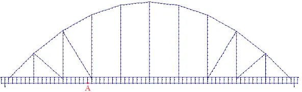
[image:8.595.185.412.326.462.2]The bridge is a bowstring arch composed of two half-decks spanning 42 m with a single track in each [5]. Figure 3 shows a view of the bridge. Each deck consists of a 40 cm thick prestressed concrete slab suspended by two lateral arches (see Figure 4). The arches are linked in the upper part by transversal girders with a rectangular hollow section and diagonals in double angles that assure the bracing of the arches.
Figure 3. São Lourenço bridge
The bridge was modeled with 2D beam elements. The influence of the deck-track composite effect in the dynamic behavior of railway bridges, due to the transmission of shear stresses between the deck and the rails at the ballasted layer, was treated in [6] and considered in the current finite element model (see Figure 4).
Figure 4. FEM model of the bridge
[image:8.595.150.446.561.652.2]1st vertical mode (1V): f = 4.25 Hz 2nd vertical mode (2V): f = 6.20 Hz
[image:9.595.89.510.77.254.2]3rd vertical mode (3V): f = 9.94 Hz
Figure 5. Mode shapes and corresponding frequencies
3.2 Dynamic model of the Alfa pendular train
[image:9.595.108.492.390.475.2]The Alfa pendular train is composed of six carriages. Each carriage has two bogies with two axles each (Figure 6). The total weight of the composition is 298.3 t, tare weight, and 323.3 t for a regular loading. The maximum weight per axle is 14.4 t and the total length of the composition is 158.90 m.
Figure 6. Alfa pendular train
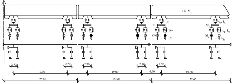
The dynamic model of the train is shown in Figure 7 and consists of rigid bodies simulating the vehicle box (mass Mc) and the bogies (mass Mb), springs with stiffness Kp (or Ks) and
dashpots with damping cp (or cs) simulating the primary (or secondary) suspensions, springs
with stiffness Kh simulating the wheel-rail contact and masses Me simulating the axles and
wheels. The train is modeled with 2D beam elements (see Figure 7).
(1)
(2) (4) (6) (3)
(5)
27,65 19,00 25,90
19,00
25,90
19,00 6,90 2,70 2,70 2,70
2,70 2,70
Mc
cp, kp cs, ks
kh Mb
[image:9.595.110.485.600.734.2]3.3 Comparison between numerical and experimental results
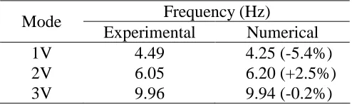
In order to validate the numerical model an experimental campaign was undertaken, which included an ambient vibration test and several measurements of passages of the Alfa pendular train [6]. The ambient vibration test was used to identify the dynamic properties of the structure, namely its natural frequencies, mode shapes and damping coefficients. The vertical accelerations at some points of the deck were measured during several passages of the Alfa pendular train. A good agreement between the natural frequencies obtained with the numerical model and the experimental values can be observed (see Table 1).
Frequency (Hz) Mode
[image:10.595.175.422.214.288.2]Experimental Numerical 1V 4.49 4.25 (-5.4%) 2V 6.05 6.20 (+2.5%) 3V 9.96 9.94 (-0.2%)
Table 1: Experimental and numerical natural frequencies
A dynamic analysis considering the train-bridge interaction was performed using the HHT method with constant average acceleration, i.e., with α = 0, β = 1/4 and γ = 1/2 [7] and a time step equal to 0.002 s. Rayleigh damping is adopted in the present study. The damping ratios of modes 1V and 3V are equal to 1.4% and 2.4%, respectively (see Table 1).
Figure 8 compares the numerical and experimental results obtained for the vertical acceleration of the deck at point A (see Figure 4), for the passage of the Alfa pendular train at 155 km/h. Both results are filtered by means of a low-pass Chebyshev (type II) filter with a cut-off frequency of 30 Hz, in accordance with the recommendations of EN1990-A2 [8].
-0.7 -0.5 -0.3 -0.1 0.1 0.3 0.5
0.0 1.0 2.0 3.0 4.0 5.0 6.0
Time (s)
A
cc
e
le
ra
ti
o
n
(
m
/s
2 )
Experimental
Numerical
Figure 8. Vertical acceleration of the deck for the passage at 155 km/h
3.4 Dynamic response of the train-bridge system
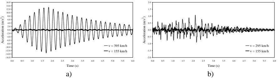
[image:10.595.80.509.451.634.2]Figure 9 shows the time histories of the vertical acceleration at the span quarter-point for the passage of the Alfa pendular train at 155 km/h and 395 km/h, and at mid-point, at 155 km/h and 295 km/h.
-16.0 -14.0 -12.0 -10.0 -8.0 -6.0 -4.0 -2.0 0.0 2.0 4.0 6.0 8.0 10.0 12.0 14.0 16.0
0.0 0.5 1.0 1.5 2.0 2.5 3.0 3.5 4.0 4.5 5.0 5.5 6.0
Time (s)
A
c
c
el
e
ra
ti
o
n
(
m
/s
2)
v = 395 km/h v = 155 km/h
-2.0 -1.5 -1.0 -0.5 0.0 0.5 1.0 1.5 2.0
0.0 0.5 1.0 1.5 2.0 2.5 3.0 3.5 4.0 4.5 5.0 5.5 6.0
Time (s)
A
c
c
el
e
ra
ti
o
n
(
m
/s
2)
v = 295 km/h v = 155 km/h
[image:11.595.74.519.139.265.2]a) b)
Figure 9. Vertical acceleration: a) quarter-point; b) mid-point
Figure 10 shows the maximum vertical acceleration for speeds ranging between 140 and 420 km/h.
0.0 2.0 4.0 6.0 8.0 10.0 12.0 14.0 16.0
140 160 180 200 220 240 260 280 300 320 340 360 380 400 420
Speed (km/h)
A
c
ce
le
ra
ti
o
n
(
m
/s
2)
0.0 0.5 1.0 1.5 2.0
140 160 180 200 220 240 260 280 300 320 340 360 380 400 420
Speed (km/h)
A
c
ce
le
ra
ti
o
n
(
m
/s
2)
[image:11.595.75.518.344.450.2]a) b)
Figure 10. Maximum vertical acceleration: a) quarter-point; b) mid-point
Resonance peaks can be observed in Figure 10 for train speeds of 395 km/h, at the span quarter-point, and for train speeds of 195 km/h, 230 km/h, 295 km/h and 310 km/h, at mid-point.
The resonance phenomena may occur for trains with regularly spaced axles, traveling at critical speeds defined by [9]
,... 4 1 , 3 1 , 2 1 ,..., 4 , 3 , 2 , 1 , =
= i
i n d (i,j)
vres j (20)
where d is the characteristic length and nj is the jth natural frequency of the bridge. The
characteristic length is a distance (many times repeated) between the vehicles or axles, that at some critical speeds may induce a periodic excitation of the bridge and cause the resonance phenomenon.
The characteristic length of the Alfa pendular train is 25.9 m (see Figure 7). According to Figure 10 and to Eq. (20), the critical speeds are: i) taking into consideration the span quarter-point and an excitation of the structure with a frequency which is equal to the mode 1V frequency (vres = 25.9×4.25/1×3.6 = 396 km/h ≈ 395 km/h); ii) considering the
mid-point and an excitation with a frequency which is equal to 1/2 and 1/3 of the frequency of
193 km/h ≈ 195 km/h) and 1/3 and 1/4 of the frequency of mode 3V (vres =25.9×9.94/3×3.6 =
309 km/h ≈ 310 km/h and vres = 25.9×9.94/4×3.6 = 232 km/h ≈ 230 km/h).
The consideration of the train-bridge interaction in the dynamic analysis is particularly useful since it allows for an accurate evaluation of the vibrations of the rail cars, and, consequently, for an assessment of the riding comfort of the passengers. Figure 11 shows the time histories of the vertical acceleration in the first and last car bodies at a speed of 155 km/h, for which there is no resonance, and at a speed of 395 km/h, for which resonance of mode 1V occurs.
-0.6 -0.4 -0.2 0.0 0.2 0.4 0.6 0.8
0.0 0.5 1.0 1.5 2.0 2.5 3.0 3.5 4.0 4.5 5.0 5.5 6.0
Time (s)
A
cc
el
er
at
io
n
(
m
/s
2)
v = 395 km/h v = 155 km/h
-2.5 -2.0 -1.5 -1.0 -0.5 0.0 0.5 1.0 1.5 2.0 2.5
0.0 0.5 1.0 1.5 2.0 2.5 3.0 3.5 4.0 4.5 5.0 5.5 6.0
Time (s)
A
cc
el
er
at
io
n
(
m
/s
2)
v = 395 km/h v = 155 km/h
[image:12.595.77.517.212.337.2]a) b)
Figure 11. Vertical acceleration: a) first car body; b) last car body
Figure 12 shows the maximum vertical acceleration in the first and last car bodies of the train for speeds ranging between 140 and 420 km/h. The maximum level of acceleration occurs in the last car body for speeds that correspond to the resonance of the bridge.
0.0 0.5 1.0 1.5 2.0 2.5
140 160 180 200 220 240 260 280 300 320 340 360 380 400 420
Speed (km/h)
A
c
ce
le
ra
ti
o
n
(
m
/s
2)
0.0 0.5 1.0 1.5 2.0 2.5
140 160 180 200 220 240 260 280 300 320 340 360 380 400 420
Speed (km/h)
A
c
ce
le
ra
ti
o
n
(
m
/s
2)
[image:12.595.80.518.430.542.2]a) b)
Figure 12. Maximum vertical acceleration: a) first car body; b) last car body
The dynamic analyses with train-bridge interaction were performed for 57 different speeds, which corresponded to a total execution time of 2624 s (≈44 min) in a 2.13 GHz personal computer. The bridge submesh has 1860 non prescribed degrees of freedom and the train submesh has 192. The total execution time of each analysis corresponds to the period between the entry of the first axle in the bridge and the exit of the last axle.
4. CONCLUSIONS
governing system of equations comprises dynamic equilibrium equations and compatibility equations. The system of linear equations that arises at each time step is efficiently solved by Gaussian elimination, by considering several submatrices and their own characteristics.
The proposed formulation is applied to the dynamic behavior of a bowstring arch bridge. The numerical model was validated with the experimental results of the ambient vibration test and those measured during several passages of the Alfa pendular train. The dynamic response of the train-bridge system was calculated for train speeds only occurring in high-speed lines, allowing for a better understanding of the behavior of the system and its resonance effects. A significant improvement in terms of efficiency could also be observed.
ACKNOWLEDGMENTS
The authors wish to acknowledge the support provided by RAVE in the context of the protocol between RAVE and FEUP. The authors also wish to acknowledge the support of the project “Risk Assessment and Management for High-Speed Rail Systems” of the MIT – Portugal Program – Transportation Systems Area. This paper reports research developed under financial support provided by "FCT - Fundação para a Ciência e Tecnologia", Portugal.
REFERENCES
[1] R. Moreno Delgado, S. M. dos Santos R. C., Modelling of railway bridge-vehicle interaction on high-speed tracks. Computers and Structures, 63, 511-523, 1997.
[2] R. Calçada, Dynamic effects on bridges due to high-speed railway traffic. MSc Thesis,
Faculty of Engineering of the University of Porto (in Portuguese), 1995.
[3] A.F.M. Azevedo, J.A.O. Barros, J.M. Sena-Cruz, A. Ventura-Gouveia, Educational software for the design of structures. Proceedings of the III Engineering
Luso-Mozambican Congress, Maputo, Mozambique, 2003, pp. 81-92 (in Portuguese), 2003. http://civil.fe.up.pt/alvaro/pdf/2003_Mocamb_Soft_Ens_Proj_Estrut.pdf
[4] A. Azevedo, S. Neves, R. Calçada, Dynamic analysis of the vehicle-structure interaction: a direct and efficient computer implementation. Proceedings of CMNE 2007 - Congress
on Numerical Methods in Engineering and XXVIII CILAMCE - Iberian Latin-American Congress on Computational Methods in Engineering, FEUP, Porto, Portugal, 2007, pp.
123 (Abstract) + 16 pages (Paper n. 1046 published on CD-ROM by APMTAC), 2007.
[5] REFER, E.P – Rede Ferroviária Nacional, Replacement of the S. Lourenço bridge at km 158,662. Design Project – Project brief, Lisboa, 2003.
[6] D. Ribeiro, R. Calçada, R. Delgado, Experimental calibration of the numerical model of the S. Lourenço railway bridge. VI Conference on Steel and Composite Construction,
Porto, Portugal (in Portuguese), 2007.
[7] T.J.R. Hughes, The Finite Element Method. Dover Publications, Inc, New York, 2000.
[8] EN1990-A2, Annex A2: Application for Bridges. European Committee for
Standardization (CEN), Brussels, 2005.
[9] EN1991-2, Actions on Structures – Part 2: General Actions – Traffic loads on bridges.