LOAD CURRENT CONTROL BASED ON LUENBERGER OBSERVER FOR THREE PHASE POWER CONVERTER SVPWM

(1)

497

A NEW MODELING OF THE LANDMARK MOVEMENT

BASED ON THE PREVIOUS MOVEMENT RESULTS TO

DETECT THE FACIAL SKETCH FEATURES

1

ARIF MUNTASA, 2MOCHAMMD KAUTSAR SOPHAN, 3MOCHAMAD HARIADI,

4

MAURIDHI HERY PURNOMO, 5KUNIO KONDO 1

Computer Science and Intelligence Laboratory, Informatics Engineering Department, Engineering Faculty, Trunojoyo University Madura,

East Java - Indonesia

2

Information System Laboratory, Informatics Engineering Department, Engineering Faculty, Trunojoyo University Madura,

East Java – Indonesia

3, 4

Electrical Engineering Department,

Industrial Engineering Faculty, Institut Teknologi Sepuluh Nopember, East Java – Indonesia

5

School of Media Science, Tokyo University of Technology Tokyo University of Technology, Katakuramachi, Hachioji, Tokyo, 192-0982 Japan

E-mail: [email protected], [email protected], [email protected],

4

[email protected], [email protected]

ABSTRACT

Deformable model is one of interest topic in biometrics. The deformable model applications have been used to detect objects included facial sketch feature images. Many methods have been discovered and developed to detect objects of deformable. However, any method can solve a problem, but raises other issues. Popular method to solve the deformable object is Active Shape Model. It is the most used to detect facial feature, but it has weakness. This method is very depended on the shape initialization. If the movement direction is not covered by training sets, then the landmark movement will be move to the undesirable direction. In this research, we proposed method to create a new modeling of the landmark movement based on the previous movement results. Four algorithms are used to improve the landmark movement when the detection process. The experimental results show that our proposed method produces the average of detection accuracies more than 90% for all scenarios.

Keywords: A New Model, Detection, The Previous Movement, Shape Model. 1. INTRODUCTION

There are two processes to recognize the human image, which are face detection and recognition. The face detection is processes to determine facial image and remove non facial image. The results of face detection are used as input in face recognition. There are three models to perform face recognition process, which are appearance [1]-[5], feature [ 6]-[8] and hybrid based recognition [9][10]. On the different modality cases, appearance based face recognition can be conducted, if they are preceded by transformation on the new space, so that they are new space [11], however they failed to recognize, when the facial sketch image model used as testing sets are the hatching images [11] [ 12].

As one of the most interest research on the last decade, facial feature detection has been conducted

(2)

ISSN: 1992-8645 www.jatit.org E-ISSN: 1817-3195

498 detection on the different modalities [19], however they failed to detect the facial features when the testing set used have slope up to 900 [20]. In this research, we proposed new algorithm to detect the facial sketch features. It is used to overcome the limitation of the previous research, where the final detection results are used as the shape initialization on the next detection process. The final results of our proposed method are superior to the previous research results [20].

2. PROPOSED METHOD

The deformable object image detection can be conducted with two ways, which is detection with and without training set. In this research, we proposed the detection model of the deformable object using the training set. The training and testing sets use the different modality. The facial image photographs are used as training set in the training process, while the facial sketch images are used as testing set in the testing process. If number of training sets used is m images, for each image has k features, and for each feature consist of n

landmark, then the feature for all training sets can be modeled as follows [20][21]













=

k m m

m

k k

k m

FT

, 2

, 1

,

, 2 2

, 2 1 , 2

, 1 2

, 1 1

, 1

,











(1)

Each training sets on the different features can consist of the different or the same number of landmarks, while for the same feature on the different training sets has the same number of landmarks. It means, for each training sets have the same number of landmarks. Detail of overall landmarks for all training set can written in the following equation

(

) (

)

(

)

(

) (

)

(

)

(

) (

)

(

)



  

 

    

 

=

n m n m m

m m m

n n

yt xt yt

xt yt xt

yt xt yt

xt yt xt

yt xt yt

xt yt xt

yt xt

, , 2

, 2 , 1 , 1 ,

, 2 , 2 2

, 2 2 , 2 1 , 2 1 , 2

, 1 , 1 2

, 1 2 , 1 1 , 1 1 , 1

, ,

,

, ,

,

, ,

,

) , (

   



 

(2)

In this research, we have trained 200 (m) the facial image photograph as training sets, for each facial image is characterized with 5 (k) features, number of landmarks used for each training sets is 27 (n). Equation (1) and (2) represents overall

landmarks used in the training set [20][21]. These landmarks will be used to obtain location of the shape initialization.

A. THE NEGATIVE MAGNITUDE OF THE

IMAGE GRADATION

The landmark movement is not moved on the original testing set, but on the testing image gradation. We proposed to create the negative magnitude of the image gradation for the landmark movement. In order to create the image gradation, we use the gaussian convolution matrix y(x,σ) as seen follows [20][21]

τ

π

σ

2

1 )

,

(

x

=

y

(3)

Where the value of τ can be defined as 2

2

2σ x

e

−

. The value of y depend on x and σ values, the Gaussian function MxN can be achieve by multiplying the Equation (3) with its derivative as seen in the following equation

( )

(

( )

)

x

y

x

y

x

H

_i _j

∂

=

σ

(

,

)

*

,

, (4)

The derivative of y(x,σ) can be calculated as seen in the following equation

)

,

(

2

1

2

1

2

1 )

,

(

2

2 2

2

2 2 2 2 2 2

σ

π

σ

π

σ

π

σ

σ σ σ

x

y

x

e

x

e

x

e

x

y

x x x

−

=













−

=













−

=













∂

=

∂

− − −

(5)

Based on the Equation (3), (4) and (5), the value of

(3)

499

( ) ( )

( )

(

)

2

2 2 2 2 2 , ) , ( ) , ( ) , ( 2 1 * 2 1 , * , , 2 2 2 2

σ

π

σ

π

σ

σ σ x y x x y x x y e x e x x y x y x H x x j i − =       − =                 −         =       ∂ ∂ = − − (6)

The parameter of x on the Gaussian function and its derivative can be repleaced with U1 and U2

respectively as written in the following equation The parameter of x on the Gaussian function and its derivative can be repleaced with U1 and U2

respectively as written in the following equation

( )

_         + − + −       − =       2 ) 1 ( 2 ) 1 ( * cos sin sin cos 2 1 M i N j U U ϕ ϕ ϕ ϕ ₍₇₎

2 )

1 (

*

)

sin(

2 )

1 (

*

)

cos(

1 1 1

+

−

+

−

=

M

i

N

j

U

ϕ

(8)

2 )

1 (

*

)

cos(

2 )

1 (

*

)

sin(

2

+

−

+

−

=

M

i

N

j

U

ϕ

(9)

where∀i, i=1 . .N dan ∀j, j=1 . . M. The matrix result from Equation (4) will be further used for convolution process

( )

x

,

y

H

,

( )

x

,

σ

f

I

=

t

⊗

ij (10)

In this case, Ix and Iy use the different values of σ

and ϕ. The gradient results of Ix and Iy can be

modeled by using the following equation

( )

i j

(

x

)

t

x

f

x

y

H

x

I

=

,

⊗

_,

,

σ

(11)

( )

i j

(

y

)

t

y

f

x

y

H

x

I

=

,

⊗

,

σ

(12)

The magnitude and its negative of the image can be easly computed by using the following equation

(

)

(

)

(

)

(

)

2

, 2 ,

,

)

,

(

,

)

,

(

y j i t x j i t

x

H

y

x

f

x

H

y

x

f

M

σ

⊗

+

⊗

=

(13)

The negative of magnitudes can be achieved by subtraction the value of 255 to M.

B. IMPROVEMENT OF TRAINING

PROCESS

Overall landmarks of the training sets have been obtained from the Equation (2), the dimension on the landmark matrix is mxn. In this case m

represents number of training sets, while number of landmarks for each training set is represented as n. Based on Equation (2), the average value of landmarks can be obtained by using the following equation

(

i i i n

)

m

j i j

i

xt

m

xt

=

= = =

∑



2 1 1 , (14)

(

i i i n

)

m j

i j

i yt yt yt

m yt

yt = = = ₌ ₌ ₌

∑

 2 1 1 , (15)

The new position of landmarks can be written













=

n m m m n n i j i j i j

xtp

r

xtp

, 2 , 1 , , 2 2 , 2 1 , 2 , 1 2 , 1 1 , 1 , , ,

)

cos(

*











ϕ

(16)













=

ytp

r

ytp

, 2 , 1 , , 2 2 , 2 1 , 2 , 1 2 , 1 1 , 1 , , ,

)

sin(

*











ϕ

(17)

Where rj,i represents square root of

2 , 2

,i ji

j

y

x

+

as seen in Equation (18), while ϕ j,i represents the new

(4)

ISSN: 1992-8645 www.jatit.org E-ISSN: 1817-3195 500 2 , 2 ,

,i ji ji

j

x

y

r

=

+

(18)

j i j i

j

φ

m

ϕ

_,

=

_,

+

(19)

The angle (φ) of the training sets and its average until the middle point (

φ

m

) can be calculated by using Equation (20) and (21)

              =                                                                                                 =         = − − − − − − − − − − n m m m n n n m n m m m m m n n n n i j i j i j xt yt xt yt xt yt xt yt xt yt xt yt xt yt xt yt xt yt xt yt , 2 , 1 , , 2 2 , 2 1 , 2 , 1 2 , 1 1 , 1 1 , , 1 2 , 2 , 1 1 , 1 , 1 , 2 , 2 1 2 , 2 2 , 2 1 1 , 2 1 , 2 1 , 1 , 1 1 2 , 1 2 , 1 1 1 , 1 1 , 1 1 , , , tan tan tan tan tan tan tan tan tan tan φ φ φ φ φ φ φ φ φ φ               (20)

(

j

)

n j i j j

m

n

m

φ



2 1 2 / 1 ,

2 /

=

∑

= (21)

The new middle point between the training sets in Equation (2) and the new position of landmarks in Equation (17) and (18) can be modeled by using the following equation













=

+

=

xp

xtp

xt

xp

, 2 , 1 , , 2 2 , 2 1 , 2 , 1 2 , 1 1 , 1 , , ,

2 









(22)













=

+

=

yp

ytp

yt

yp

, 2 , 1 , , 2 2 , 2 1 , 2 , 1 2 , 1 1 , 1 , , ,

2 









(23)

The average of the new middle point can be computed by using the following equation

(

n

)

m j i j i

xp

n

xp



2 1 1 ,

1 =

=

∑

= (24)

(

n

)

m j i j i

yp

n

yp



2 1 1 ,

1 =

=

∑

= (25)

The zero means of the new middle point can be calculated by subtraction the Equation (22) and (23) to their average as seen in Equation (24) and (25). To simplify the zero means calculation, it is necessary to duplicate the results of Equation (24) and (25) as many as m rows. The zero means can be calculated as seen in the following equation

(5)

501













=













−













=

n m m m n n m n m m n n n m m m n n

yv

yp

yv

, 2 , 1 , , 2 2 , 2 1 , 2 , 1 2 , 1 1 , 1 , , 2 , 1 2 , 2 , 2 2 , 1 1 , 1 , 2 1 , 1 , 2 , 1 , , 2 2 , 2 1 , 2 , 1 2 , 1 1 , 1



























(27)

In this research, we have proposed to improve the landmark variation based on deviation standard and its zero means. The deviation maximum value depends on the minimum value and deviation standard of xv. Similarly with the deviation maximum value also depends on the maximum value and deviation standard of yv. They can be determined as seen in the following equation

∑

= =

+

=

_m j j m j j i j i

xv

Std

xv

Std

xv

x

SMin

1 1 2 ,

_

)

min(

_

σ

(28)

∑

= =

−

=

_m j j m j j i j i

xv

Std

xv

Std

xv

x

SMax

1 1 2 ,

_

)

max(

_

σ

(29)

∑

= = + = _m j j m j j i j i yv Std yv Std yv y SMin 1 1 2 , _ _ ) min(

_

σ

(30)

∑

= =

−

=

_m j j m j j i j i

yv

Std

yv

Std

yv

y

SMax

1 1 2 ,

_

)

max(

_

σ

(31)

Where Std_xvj and Std_yvj represent the deviation

standard values of xv and yv as seen in the following equation

(

)

2

1 , ,

1

1 _

∑

=

−

=

n i i j i j

j

xv

n

xv

Std

(32)

(

)

2

1 , ,

1

1 _

∑

=

−

=

n i i j i j

j

yv

n

yv

Std

(33)

While

xv

j and

yv

_jare the average of xv and yv

∑

=

n i i j j

xv

n

xv

1 ,

1

(34)

∑

=

n i i j j

yv

n

yv

1 ,

1

(35)

The new landmark variation is landmark improvement of Equation (26) and (27). They can be obtained by using the following equation













=

+

=

x

xv

x

, 2 , 1 , , 2 2 , 2 1 , 2 , 1 2 , 1 1 , 1 , , ,

σ











(36)













=

+

=

y

xv

y

, 2 , 1 , , 2 2 , 2 1 , 2 , 1 2 , 1 1 , 1 , , ,

σ











(37)

C. DETERMINATION OF THE SHAPE

INITIALIZATION BASED ON THE TRAINING PROCESS RESULTS

The shape initialization plays important role in the detection process. Error in determining the shape initialization will have an impact on the final result of the detection process. The closer the shape initialization to the corresponding features, the faster the process to find the corresponding features [20][21]. In order to obtain the shape initialization, it is necessary to conduct the training process

i

x

c

i

σx

XP

i

(6)

ISSN: 1992-8645 www.jatit.org E-ISSN: 1817-3195 502 i

y

c

i

σy

YP

i

YL

=

+

.

∆

δ

(39)

Where

XP

and

YP

represent the normalized average of xtp and ytp. For both

XP

and

YP

have the single value as seen follows

              =               = n m m m n n n m m m n n XP XP XP XP XP XP XP XP XP xtp xtp xtp xtp xtp xtp xtp xtp xtp xtp XP , 2 , 1 , , 2 2 , 2 1 , 2 , 1 2 , 1 1 , 1 , 2 , 1 , , 2 2 , 2 1 , 2 , 1 2 , 1 1 , 1 ) max( 1 *               (40)

∑∑

= =

=

m j n i i j

XP

n

m

XP

1 1 ,

*

1

(41)               =               = n m m m n n n m m m n n YP YP YP YP YP YP YP YP YP ytp ytp ytp ytp ytp ytp ytp ytp ytp ytp YP , 2 , 1 , , 2 2 , 2 1 , 2 , 1 2 , 1 1 , 1 , 2 , 1 , , 2 2 , 2 1 , 2 , 1 2 , 1 1 , 1 ) max( 1 *               (42)

∑∑

= =

=

m j n i i j

YP

n

m

YP

1 1 ,

*

1

(43) The following is an example of the shape initialization. It will be placed in accordance with the results of equation (38) and (39). Figure (1) show transformation of the shape initialization process

Fig.1. Transformation to the Shape Initialization

To calculate the deviation standard of the landmark variation, it is necessary to compute the average of the landmark variation. It can be calculated by using the following equation

m

x

m j i j i

∑

=

1 ,

σ

(44)

m

y

m j i j i

∑

=

1 ,

σ

(45)

The deviation standard of the landmark variation can be calculated by using the following equation

(

)

∑

=

−

=

n i i j i j

x

n

x

Std

1 2 , ,

1

1 _

σ

(46)

(

)

∑

=

−

=

n i i j i j

y

n

y

Std

1 2 , ,

1

1 _

σ

(47)

The middle point of the landmark variation average can be easily calculated by using the following equation

2 min

max

(

xv

)

(

xv

)

xt

i i i

−

=

∆

(48)

2 min

max

(

yv

)

(

yv

)

yt

i i i

−

=

∆

(49)

And the middle point of the deviation maximum and minimum can be computed by using the following equation

2 )

_

(

_i _i

i

x

Min

Simp

x

Max

Simp

x

σ

δ

=

−

∆

(50)

2 )

_

(

_i _i

i

y

Min

Simp

y

Max

Simp

y

σ

δ

=

−

∆

(51)

The results of training process will be used to detect the sketch facial feature, which are update the landmark variation values of x and y using Equation (24), (25), (36) and (37), while update the new value using Equation (28), (29), (30) and (31)

D. A NEW MODEL OF THE DETECTION

PROCESS

(7)

503 is put on the image gradation. It moves to the corresponding feature depend on the greatest gradation. It will move close to the edge of features. To move the shape toward the corresponding feature, we proposed the similarity Affine as seen in the following equation













+













=













y x i i i i

T

YL

XL

Af

NewY

NewX

*

(52) Where













−

=

)

cos(

*

)

sin(

*

)

sin(

*

)

cos(

*

ϕ

sY

sX

Af

The values of scallingX and scallingY have range between 0.8 until 1.2, whereas the value of ϕ has range between -150 until 150 and we utilize

σ

x

i for

Tx and

σ

y

_i for Ty. The results of Equation (38) and

(39) are used as input in Equation (52). The results of Equation (52) will be used to update the value of

xt and yt, which are xti=NewXi and yti=NewYi.

These values will be evaluated by using the following equation

( ) (

)

( )(

)

( )(

)

( ) (

)

( )(

)

( )(

)

( ) (

)

( )(

)

( )(

)

( ) (

)

( )(

)

( )(

)

( ) (

)

( )(

)

( )(

)

( ) (

)

( )(

)

( )(

)

























−

+

≤

−

+

−

+













−

+

>

−

+

−

+

=

∆

+ + + + + + + + + + + + + + + + + + 1 1 2 1 2 1 1 2 1 2 1 1 2 1 2 1 1 2 1 2 1 1 2 1 2 1 1 2 1 2

2

i i i i i i i i i i i i i i i i i i i i i i i i i i i i i i i i i i i i

xt

yt

if

xt

yt

if

yt

xy

(53)

The improvement of the gradient value can be modeled by using the following equation

( ) (

)

( )(

)

(

) (

)

i

i i i i i i i i i xt yt yt xt xt xt xt xt xt xt + − + − − + = + + + + 2 1 2 1 1 2 1 2 2

α (54)

( ) (

)

( )(

)

(

) (

)

i

i i i i i i i i i yt yt yt xt xt yt yt yt yt yt + − + − − + = + + + + 2 1 2 1 1 2 1 2 2

α (55)

The gradient values average along the line can be written by using the following equation

( ) ( )

(

) (

)

2

1 2 1 1 1 1

)

(

+ + + + + =

−

+

−

=

∑

+ + i i i i yt yt xt xt l l

yt

xt

G

i i i i (56) ( ) ( )

(

) (

)

2

1 2 1 1 1 1

)

(

+ + + + + =

−

+

−

=

∑

+ + i i i i yt yt xt xt l l

yt

xt

yt

G

i i i i (57)

To evaluate the gradient value, we proposed to use the previous research (Arif Dkk., 2009c) as seen in the following rules

If

xy

(

)

(

1

)

2

1

2

1

−

+

−

<

(8)

504

( ) ( )

(

) (

)

(

) (

)

(

1 1

)

2 1 2

1

2 1 2

1 2

1 1

1 )

(

)

(

)

1 )

(

)

(

*

)

(

1 1

+ +

+ + +

=

+

−

+

−

+

−

+

−

=

∑

+ +

i i i

i i

i

i i i

i i

i

yt yt xt xt

l l

yt

xt

yt

xt

yt

xt

yt

xt

LG

i i i i

(58)

( ) ( )

(

) (

)

(

) (

)

(

1 1

)

2 1 2

1

2 1 2

1 2

1 1

1 )

(

)

(

)

1 )

(

)

(

*

)

(

1 1

+ +

+ + +

=

+

−

+

−

+

−

+

−

=

∑

+ +

i i i

i i

i

i i i

i i

i

yt yt xt xt

l l

yt

xt

yt

xt

yt

xt

yt

xt

yt

LG

i i i i

(59)

Else

( ) ( )

(

) (

)

2

1 2

1 1

)

(

+ +

+ + +

=

−

+

−

=

∑

+ +

i i i

i

yt yt xt xt

l l

yt

xt

LG

i i i i

(60)

( ) ( )

(

) (

)

2

1 2

1 1

)

(

+ +

+ + +

=

−

+

−

=

∑

+ +

i i i

i

yt yt xt xt

l l

yt

xt

yt

LG

i i i i

(61)

We proposed 4 algorithms to conduct the facial sketch detection processes, which are algorithm used to detect facial sketch for each feature as seen in Algorithm 1. Algorithm 2 is used to perform the facial sketch detection for all features as seen in algorithm 2. To improve the detection process of Algorithm 2, we proposed Algorithm 3 to perform it. In order to produce landmark locations in accordance with the position of features, it is necessary to move the landmarks based on the results of Algorithm 3 as seen in Algorithm 4.

Algorithm 1 The Facial Sketch Detection for each Feature

1. Read ‘feature’ file

2. While |xtj-xtj+1|>xThreshold and |ytj-ytj+1|>yThreshold do step 3

3. ∀a, a∈1..K do step 4

4. Do Algorithm 2

5. P1clusterpoint(a,1) p2clusterpoint(a,2) 6. ∀i, i∈1..n do step 7

7. ∀j, j∈p1..p2 do step 8 and 9

8. Update the landmark variation of x using equation (24) and (36)

9. Update the landmark variation of y using equation (25) and (37)

(9)

505

Algorithm 2 The Facial Sketch Detection for all Features

1. ∀Tx where Tx∈TLx..TUx.do step 2

2. ∀Ty1 where Ty∈TLy..TUy. do step 3

3. ∀ScallingX where ScallingX∈ ScallingXL.. ScallingXU do step 4

4. ∀ScallingY where ScallingY∈ ScallingYL.. ScallingYU do step 5

5. ∀ϕ where ∀ϕ∈ϕL ..ϕU do step 6

6. P1clusterpoint(a,1) p2clusterpoint(a,2) 7. ∀i, i∈1..n do step 8

8. ∀j, j∈p1..p2do step 9

9. Determine the new landmark Using Equation (52)

10. Evaluate the landmark value along the line using Equation (53)

until (57)

11. Calculate the image gradient value along line

12. Evaluate the image gradient value using Equation (58) until (61)

Algorithm 3 Feature Detection Improvement

1. Read the new landmark from detection results using the 1st and

2nd algorithm.

2. Read ‘feature’ file

3. While |xtj-xtj+1|>xThreshold and |ytj-ytj+1|>yThreshold do the 4th

step

4. ∀a, a∈1..K do the 5th step

5. Do the 4th Algorithm

6. P1clusterpoint(a,1) p2clusterpoint(a,2) 7. ∀i, i∈1..n do the 8th step

8. ∀p, p∈p1..p2 do the 8th and 9th steps

9. Update the landmark variation value of x using Equation (24)

and (36)

10. Update the landmark variation value of y using Equation (25)

and (37)

11. Compute the new landmark using equation (52)

12. Update the value of xti and yti, where x1xti+Tx dan y1yti+Ty.

13. If p<p2 do

a. x2 xti+1 + Tx

b. y2 yti+1 + Ty

c. evaluate the landmark along line using Equation (53)

until (61)

14. If p>=p2 do

a. x2 xti+1 + Tx

b. y2 yti+1 + Ty

c. evaluate the landmark along line using Equation (53)

until (61)

d. Update the gradient value as result from Equation

(53) until (61)

15. Update the new value using Equation (28) until (31)

(10)

506

Algorithma 4 The Last Movement to Detect Features

1. ∀Tx where Tx∈TLx..TUx do the 2nd step

2. ∀Ty where Ty∈TLy..TUy do the 3rd step

3. ∀ScallingX where ScallingX∈ ScallingXL.. ScallingXU do the 4th step

4. ∀ScallingY where ScallingY∈ ScallingYL.. ScallingYU do the 5th step

5. ∀ϕ where ∀ϕ∈ϕL ..ϕU do the 6th step

6. p1=clusterpoint(a,1) p2=clusterpoint(a,2)

7. ∀i, i∈1..n do the 8th step

8. ∀p, p∈p1..p2do the 9 th

, 10th, 11st, 12nd, and 13rd

9. Determine the new landmarks using Equation (52)

10. Update the value of xti and yti, where x1xti+Tx and

y1yti+Ty.

11. If p<p2 do

a. x2 xti+1 + Tx

b. y2 yti+1 + Ty

c. evaluate the landmark along line using Equation (53) until (61)

12. If p>=p2 do

a. x2 xti+1 + Tx

b. y2 yti+1 + Ty

c. evaluate the landmark along line using Equation (53) until (61)

d. Update the gradient value as result from Equation (53) until (61)

13. Update the new value using Equation (28) until (31)

14. Determine the new landmark value using Equation (52)

3. EXPERIMENTAL RESULTS AND

ANALYSIS

In this research, we utilized 100 face images tilted toward the left and 100 images tilted to the right as training sets. We have marked 27 important points as landmark, which are 4 landmarks on the eyebrow, 5 landmarks for eye, 6 landmarks for each the noose, the lips and the face curvature respectively. 400

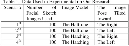
[image:10.612.195.455.590.684.2]

facial sketch images have been used as testing set, which are 200 the halftone and 200 the hatching facial sketch images with tilted 200 until 900. We have conducted experiments in 4 scenarios. For each scenario have used 100 facial sketch images with different model and pose as seen in Table 1.

Table 1. Data Used in Experimental on Our Research Scenario Number of

Facial Sketch Images Used

Image Model The Image Pose Tilted toward

1st 100 The Halftone The Right 2nd 100 The Halftone The Left

(11)

[image:11.612.316.530.75.208.2]

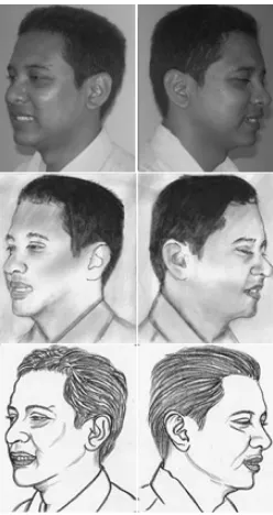
507 The testing sets and the training sets have the different modalities. We use photograph images as the training set and sketch image as the testing sets. Two photograph images of the different person have smaller distance than two images of the same persons, those are photograph and sketch. The training and the testing set samples for the halftone and the hatching facial sketch image can be seen in Figure (2).

Fig.2. Photograph image as the training sets (1st row), the Halftone (2nd row) and the Hatching (3rd

row) as the testing Sets

[image:11.612.138.262.211.445.2]

Sample of experimental results on the 1st and the 2nd scenarios can be seen in Figure (3)

Fig. 3. Experimental Results on the 1st (the 1st row) and the 2nd (the 2nd row) Scenarios Figure (4) shows sample of the experimental results on the 3rd and the 4th scenarios.

Fig. 4. Experimental Results on the 3rd (the 1st row) and the 4th (the 2nd row) Scenarios

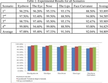
The experimental results for all scenarios can be seen in Table 2. On the 1st and 3rd scenarios, the experimental results showed that the highest detection accuracy has occurred on the eyebrow feature, while on the face curvature has yielded the lowest detection accuracy. The error detection on the face curvature was the most caused by the landmark movement tend to follow the 2D-Gauss gradation results. The error of landmark detection on the face curvature has caused the shape change of the face curvature as seen in Figure (5).

On the 2nd scenario, the experimental results showed that the lowest detection accuracy has occurred on the lips feature, while the highest detection accuracy has occurred on the nose feature. The same results also occurred on the 4th scenario, where the eyebrow and the nose features have been detected with the highest accuracy, while the detection results on the lips feature produce the lowest accuracy. The most common error on the 2nd and the 4th scenarios are caused by scratches that were around the feature. The results of gradation formation using 2D-Gaussian functions also follow the object produced by Sketcher, so the accuracy of feature detection is also very dependent on the sketch produced by Sketcher. Scratches around the lips made livelier, but the results have given effect decreasing in detection accuracy as seen in Figure (6).

[image:11.612.94.304.536.662.2] [image:11.612.330.517.588.703.2]

(12)

[image:12.612.98.304.76.232.2]

508 Fig 6. The Detection Error on the Lips Feature Our experimental results have been compared with previous research, which are the Mixture

[image:12.612.127.480.295.567.2]

Model, Landmark Variation Improvement method and Geometrical Structured Base. On the 1st and 2nd scenarios, the detection results of our proposed method is superior to the Mixture Model and Landmark Variation Improvement method as seen in Figure (6) and (7). Our proposed method is also superior to the Mixture Model and the Geometrical Structured Base method, except on the face curvature feature as seen Figure (9), while on the 4th scenario our proposed method produces detection accuracies higher than the Mixture Model and the Geometrical Structured Base, it can be described in Figure (10)

Table 2. Experimental Results for all Scenarios

Scenario Eyebrow The Eye Nose The Lips Face Curvature Average 1st 96.25% 96.20% 95.33% 93.17% 88.50% 93.89% 2nd 97.50% 93.40% 99.50% 88.50% 94.00% 94.58% 3rd 98.75% 97.40% 95.50% 95.17% 92.67% 95.90% 4th 99.00% 94.60% 99.00% 88.50% 93.00% 94.82% Average 97.88% 95.40% 97.33% 91.34% 92.04% 94.80%

(13)

[image:13.612.94.529.70.226.2]

509

[image:13.612.168.450.281.423.2]

Fig 8. The Comparison Results of Detection Accuracy between Mixture Model [12], Landmark Variation Improvement [21] and the 2nd Scenario of Proposed Method

Fig 9. The Comparison Results of Detection Accuracy between Mixture Model [12], Geometrical Structured Base [20] and the 3rd Scenario of Proposed Method

Fig 10. The Comparison Results of Detection Accuracy between Mixture Model [12], Geometrical Structured Base [20] and the 4th Scenario of Proposed Method

4. CONCLUSION

Our proposed method has proved that the average of the detection accuracies more than 90% for all scenarios and features. The highest average of detection accuracies occurred on the eyebrow

[image:13.612.165.452.470.624.2]

(14)

510 our proposed method is superior to other methods such as the Mixture Model, Landmark Variation Improvement method and Geometrical Structured Base. However, our proposed also has weakness in feature detection. The detection results of our proposed method are also depended on the sketch results. If the results of facial sketch contains many scratches, then the results of gradation formation using 2D-Gaussian also produces many scratches. The more scratches produced in image, the lower detection accuracies yielded. For the next research, it is necessary to improve algorithm to remove many scratches on the testing sets before detection process.

REFERENCES

[1] X. He, S. Yan, Y. Hu, P. Niyogi, and H.-J. Zhang. Face recognition using laplacianfaces. IEEE Transactions on PatternAnalysis and Machine Intelligence, , 2005, 27(3):328–340.

[2] Cai, D., He, X., and Han, J. Using Graph Model for Face Analysis, University of Illinois at Urbana-Champaign and University of Chicago, 2005.

[3]. Kokiopoulou, E. and Saad, Y. Orthogonal Neighborhood Preserving Projections, University of Minnesota, Minneapolis, 2004.

[4] Arif Muntasa, Mochamad Hariadi, Mauridhi Hery Purnomo, "Automatic Eigenface Selection For Face Recognition", The 9th Seminar on Intelligent Technology and Its Applications, ITS Surabaya, 2008, 29 – 34. [5]. Arif Muntasa, Mochammd Kautsar Sophan,

Indah Agustien S., Mauridhy Heri P., “ Appearance Global And Local Structural Fusion For Face Image Recognition”, 2011, Telkomnika Journal Vol 9, No. 1. Pp 125-132.

[6]. Pan, G.; Han, S.; Wu, Z. & Wang, Y., “3D face recognition using mapped depth images”, Proceedings of IEEE Workshop on Face Recognition Grand Challenge Experiments, June 2005

[7]. C. Kotropoulos, A. Tefas, and I. Pitas, “Frontal Face Authentication Using Morphological Elastic Graph Matching,” IEEE Trans. Image Processing, vol. 9, pp. 555-560, April 2000.

[8]. Mian, A. S., Bennamoun, M., & Owens, R. A., “Face recognition using 2D and 3D multimodal local features”. In International

symposium on visual computing, 2006, pp. 860–870

[9]. Xu, C.; Wang, Y.; Tan, t. & Quan, L., “Automatic 3D face recognition combining global geometric features with local shape variation information”, Proceedings of Sixth International Conference on Automated Face and Gesture Recognition, May 2004, pp.308–313

[10]. Mian, A. S., Bennamoun, M., & Owens, R. A., “An efficient multimodal 2D–3D hybrid approach to automatic face recognition”.

IEEE Transactions on Pattern Analysis and Machine Intelligence, 2007, Vol 29, No 11, pp. 1927–1943.

[11]. Arif Muntasa, “New Approach: Dominant and Additional Features Selection Based on Two Dimensional-Discrete Cosine Transform for Face Sketch Recognition”, International Journal of Image Processing (IJIP), 2010, Vol. 4, No. 4, pp. 368-376 [12]. Arif Muntasa, Mochammad Kautsar Sophan,

Mauridhi Hery P., Kondo Kunio, “The Hatching Facial Sketch Representation based on Mixture Model”, IJACT: International Journal of Advancements in Computing Technology, 2011, Vol. 4, No. 3, pp. 239-249.

[13]. Christos Davatzikos, Xiaodong Tao, and Dinggang Shen, "Hierarchical Active Shape Models, Using the Wavelet Transform", IEEE Transaction on Medical Imaging, 2003, VOL. 22, NO. 3, pp. 414-423

[14]. Bram van Ginneken, Alejandro F. Frangi, Joes J. Staal, Bart M. ter Haar Romeny, and Max A. Viergever, "Active Shape Model Segmentation With Optimal Features", IEEE Transactions on Medical Images, 2002, Vol. 21, No. 8, pp. 924-933.

[15]. D. DeCarlo and D. Metaxas, “Optical Flow Constraints on Deformable Models with Applications to Face Tracking,” International Journal Computer Vision, vol. 38, no. 2, pp. 99-127, July 2000.

[16]. N.Babaii Rizvandi, A. Pižurica, W. Philips, “Deformable Shape Description Using Active Shape Model (ASM)", In Proc. of the 18th ProRISC workshop on Circuits, Systems and Signal Processing (ProRISC 2007), Veldhoven, pp. 191-196.

(15)

511 linked active appearance models", Proc. Medical Image Understanding and Analysis, 2006, Vol. 2, pp.120-4.

[18]. Arif Muntasa, Hariadi M, Mauridhi Hery Purnomo, “A New Formulation of Face Sketch Multiple Features Detection Using Pyramid Parameter Model and Simultaneously Landmark Movement”,

International Journal of Computer Science Network and Security, 2009, Vol 9. No 9, pp. 249-260

[19]. Xiaoou Tang and Xiaogang Wang, “Face Sketch Synthesis and Recognition”, Proceedings of the Ninth IEEE International Conference on Computer Vision (ICCV), 2003, Volume Set 0-7695-1950-4.

[20]. Arif Muntasa, Mochammd Kautsar Sophan, “Geometrical Structure Based the Greatest Gradation for the Hatching Facial Sketch Features Detection”, International Conference on Computer Science, Information System & Communication Technologies. September 2012, Bangkok-Thailand, pp.60-68.