DYNAMIC TRAFFIC LIGHT CONTROL FOR INTELLIGENT
MOBILITY IN SMART CITIES
BEN AHMED Mohamed, GHADI Abderrahim, BOUDHIR Anouar, BOUHORMA Mohammed, BEN AHMED Kaoutar
LIST laboratory, Abdelmalek Essaadi University
Computer Sciences department, Faculty of Sciences and Techniques of Tangier - Morocco
E-mail: [email protected], [email protected], [email protected] [email protected]
ABSTRACT
Intelligent Mobility is the most important pillar in the approach of the smart city because the urban road traffic is the heart of many problems in many fields, such as economics or ecology. Therefore, the Intelligent Transportation Systems (ITS) have emerged to best optimize the expenditure of the user on often complex road networks. In this paper, after studying the backgrounds of such systems, we suggest a dynamic traffic lights control through the use of statistical multiplexing technique based on V2I in Vanets. We will see that this architecture can be flexible within the framework of ITS and participate in low cost to obtain interesting results.
The simulation results prove the efficiency of the dynamic automatic traffic light control system in an urban area and the comparison of the proposed system with other systems in the scientific literature improve the effectiveness of our approach
Keywords: Smart city, Vanet,NS2, ITS, SDTM
1. INTRODUCTION
The urban road traffic has dramatically grown recently increasing the severity of a number of issues such as traffic jams, accidents, and pollution. To an employer, congestion (Fig.1) means lost worker productivity, trade opportunities, delivery delays, and increased costs. A city is where traffic flows, it needs to make mobility smarter to overcome efficiency, safety and environmental challenges faced today. Smart mobility is one of the eight key factors that define a smart city according to Frost & Sullivan, together with the other seven aspects shape the cities of the future. Inside these digital, interactive and connected cities, so-called smart cities, Information and Communications Technologies (ICTs) are leveraged to have real-time Information effectively exchanged between mobility infrastructure devices (sensors, vehicles, digital technologies etc.) in order to respond to different urban transportation problems such as congestions, disaster planning, eco problems, among others. Governments, companies and citizens as well must stand up to ensure the development of smart mobility. Hence, sustainable, innovative and safe transportation systems will improve logistics, reduce costs and
respect the environment consequently will improve citizens’ quality of life and productivity which is the main objective of smart cities.
Resolving congestion problems is feasible not only by physically constructing new facilities and policies but also by building information technology transportation management systems (ITS).The road traffic management is in the field of (ITS), designed to provide tools and models to
manage risks by reactive equipment. The
implementation of such systems will have multiple objectives, including the thinning traffic incident
detection, the real-time traffic monitoring,
information dissemination or variables instructions to motorists and the corresponding reduction in pollution and noise. Many traffic light systems operate on a timing mechanism that changes the
Figure 1: Complex scenario of traffic promoting congestion
An intelligent traffic light system senses the presence or absence of vehicles and reacts accordingly. The idea behind intelligent traffic systems is that drivers will not spend unnecessary time waiting for the traffic lights to change. An intelligent traffic system detects traffic in many different ways [1]. The older system uses weight as a trigger mechanism [2]. Current traffic systems react to motion to triggers the light changes. Once the infrared object detector picks up the presence of a car, a switch causes the lights to change. In order to accomplish this algorithms are used to govern the actions of the traffic system. While there are many different programming languages today, some programming concepts are universal in Boolean Logic.
In this paper, we propose a traffic light controller that can deal with the traffic congestion appropriately. Based on the statistical multiplexing method it uses as input variable a degree of traffic congestion of upper roads, which vehicles on a crossroad are proceeding to. We compared and analyzed the fixed traffic signal controller and the proposed system by using the delay time and the proportion of passed vehicles to entered vehicles. As a result of comparison, the proposed controller showed more enhanced performance than the fixed traffic signal controller.
2. RELATED WORKS
Due to the importance of the ITS topics, several works was focused on this field and area. Authors in [3], discuss how optimal and suboptimal traffic light switching schemes with possible variation of cycle as a function of time. Binbin Zhou & al [4] propose an adaptive traffic light control algorithm to adjust the sequence and length of traffic lights in accordance with the real time traffic detected. Their algorithm considers a number of traffic factors such as traffic volume, waiting
time, vehicle density to determine green light sequence and the optimal green light length.
In [5], authors used Wireless Sensor Network (WSN) as a tool to instrument and control traffic signals roadways, and a traffic controller to control the operation of the traffic infrastructure. Malik & al [6], proposed an architecture system which is classified into three layers; the wireless sensor network, the localized traffic flow model policy, and the higher level coordination of the traffic lights agents that manages its intersection by controlling its traffic lights. Holger.p& al [7], presents an organic approach to traffic light control in urban areas that exhibits adaptation and learning capabilities, allowing traffic lights to autonomously react on changing traffic conditions.
3. THE TRAFFIC LIGHT CONTROL
SYSTEM
There are usually two different modes adopted by most nations on the planet: fixed time and dynamic control. Let's take them one a time and see the differences. A fixed time traffic light control system is that boring and old-fashioned way in which traffic lights are configured to turn on the green color after a given period of time, usually around 30 seconds, but this may very well vary depending on traffic values and region. The fixed time traffic light control systems relied on an electro-mechanical signal controller, it's a less complicated controller with components that can move, but also with dial timers to be able to keep a specific color for a given period of time.
Figure 2: Basic concept of Smart Traffic Light Controller
4. STATISTICAL MULTIPLEXING
Statistical multiplexing dynamically
allocates bandwidth to each channel on an as-needed basis. This is in contrast to time-division multiplexing (TDM) techniques, in which quiet devices use up a portion of the multiplexed data stream, filling it with empty packets. Statistical multiplexing allocates bandwidth only to channels that are currently transmitting. It packages the data from the active channels into packets and dynamically feeds them into the output channel, usually on a FIFO (first in, first out) basis, but it’s also able to allocate extra bandwidth to specific input channels.
4.1 The scalar conservation law
A scalar conservation law [8] in one space dimension is a first order partial differential equation of the form
(1.1)
Here is called the conserved
quantity, while f is the flux.
The variable t denotes time, while x is the one-dimensional space variable.
Equations of this type often describe transport phenomena. Integrating (1.1) over a given interval [a, b] one obtains
In other words, the quantity u is neither created nor destroyed: the total amount of u
[image:3.595.73.514.81.312.2] [image:3.595.75.305.103.301.2]containedinside any given interval [a, b] can change only due to the flow of u across boundary points (fig. 3).
Figure 3: Flow across two points.
Figure 3: Flow across two points.
Using the chain rule, (1.1) can be written in the quasi linear form
(1.2)
Where is the derivative of . For
smooth solutions, the two equations (1.1) and (1.2)
are entirely equivalent. However, if has a jump at a point ε , the left hand side of (1.2) will contain the
product of a discontinuous function with the
distributional derivative , which in this case
contains a Dirac mass at the point ε. In general, such a product is not well defined. Hence (1.2) is meaningful only within a class of continuous functions. On the other hand, working with the equation in divergence form (1.1) allows us to
consider discontinuous solutions as well,
interpreted in distributional sense.
A function will be called a weak
solution of (1.1) provided that
(1.3)
for every continuously differentiable function with
compact support
Notice that (1.3) is meaningful as soon as both u and f(u) are locally integrable in the t-x plane.
4.2 The conservation law Application in the
traffic flow.
Let be the density of cars on roads near to
the intersecting at the point x at time t. For
ρ is continuous and that the velocity of the cars depends only on their density:
with
Given any two points a, b on the highway, the number of cars between a and b therefore varies according to the law
(1.4)
Figure 4: The density of cars can be described by a conservation law.
Since (1.4) holds for all a, b, this leads to the
conservation law where ρ
is the conserved quantity and is
the flux function.
5. ALGORITHM
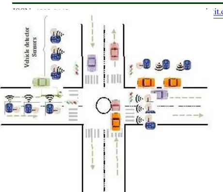
The proposed algorithm is designed to manage the traffic cycle which can be changed dynamically by giving priority to vehicles in the less dense road to facilitate the efficient traffic control at certain junction. This algorithm is based on the statistical information using the conservation law of vehicles in the four road parts and using a hierarchical wireless sensor network (fig. 5). This also can be extended to multiple crossroads control.
.
Figure 5: illustration of proposed algorithm method
The traffic controller algorithm is defined as follow:
Algorithm:
Let NA , NA’, NB,NB’, numbers of vehicles, respectively, in
roads A,A’,B and B’
density of car at time t and position xi
inroad jWhere j= {A,A’,B,B’}
mean_delay(i,j): the mean time of evacuation from roads (A,A’) or (B,B’)
min_time_evacuation:minimum time of evacuation froma road (for yellow light)
Do
Sensors road’s Start detecting vehicles Achieving accounted values to de CH Computing min (sum(NA,NA’),sum(NB,NB’))
Computing for every value of j at time t mean_delay(k,k’)=
If sum(NA,NA’)> sum(NB,NB’)
Then
mean_delay(B,B’)= mean_delay(B,B’)/2 Else
mean_delay(A,A’)= mean_delay(A,A’)/2 End if.
If sum( , ’) >= sum( , ’)
Then
(B_light and B’_light): G until delay=( +
)*mean_delay_(B,B’)
( A_light and A’_light): R until delay=( + ))*mean_delay(B,B’)+min_time_evacuation
( B_light and B’_light):Y until delay= min_time_evacuation
( A_light and A’_light): G until delay=( + )
*mean_delay(A,A’)
(B_light and B’_light): R until delay=( + )
*mean_delay(A,A’)+min_time_evacuation
( A_light and A’_light):Y until delay= min_time_evacuation
Else
( A_light and A’_light): G until delay=( +
)*mean_delay(A,A’)
( B_light and B’_light): R until delay=( + )
*mean_delay(A,A’)+min_time_evacuation
( A_light and A’_light):Y until delay= mean_time_evacuation
( B_light and B’_light): G until delay=( +
)*mean_delay(B,B’)
( A_light and A’_light): R until delay= ( + )
*mean_delay(B,B’)+min_time_evacuation
( B_light and B’_light):Y until delay= min_time_evacuation
End if.
Loop.
5.1 Discussion& Analysis
In this algorithm, we proposed a dynamic traffic light commutation based on the conservation law and the density of road and the incremental values of vehicles given by sensor detector. The basic idea is to reduce traffic by giving priority to the least dense route to evacuate the smaller number vehicle, before opening the way to the highest road density in term of vehicles. On one hand, this solution is based on the law of conservation and the density function, and on the other hand, by using the number of vehicles provided by the sensors to solve the problem higher density road proceeding to the reduction of time of the other side road traffic in to the half mean time of evacuation.
The basic idea behind this work is to adapt the light variation to quantity of vehicles in the segment [xi,b] (Fig.5). In fact, the system compute, at time t, the number of vehicles between xi and b in both sides (A,A’) and (B,B’), using the low of conservation , respectively the values [
+ ] and [ + ],then turn on the
green light to the corresponding minimal mentioned values. The crucial decision to this is to evacuate the road containing the less number of vehicles before the other side, in order to give more time to the dense road for the evacuation. Moreover, when the values of sensors related to the number of vehicles (for example) in roads (A,A’) is more the same values in roads (B,B’), the time dedicated to the green light is divided by 2, to accelerate the evacuation of the selected road having a green light.The performance of this idea is to reduce the waiting time in the selected road (having green light) to be evacuated quickly before giving enough evacuation time to the other side.
In the opposite situation, if we turn on the green light to the dense roads [to the roads (B,B’)], the vehicles in the other side [roads (A,A’)] will
wait all the time (( + )
*mean_delay(B,B’)+min_time_evacuation) reserved to the evacuation of the dense roads (B,B’), before taking their time to evacuate roads
(A,A’) (( + ) *mean_delay(A,A’)).
The last situation consume more waiting time for vehicles in roads (A,A’). Consequently, the ideal is to rapidly evacuate the roads (A,A’) then roads (B,B’). Acting so, the vehicles in roads (B,B’) will wait (less time) just for the time ((
+ ) *mean_delay(A,A’)).
Example:
1st case of study: (Evacuation of the less dense road) N um b er of ve hi cl es M ea n ev ac ua tion tim e f or 1 ve hi cl e Me a n e v a c u a ti o n t im e fo r a R o a d Li ght W a iti ng tim e G loba l W a iti ng tim e R o ad s
(A,A’) 10 3s 10*3s
=30s 30s
120s
(B,B’) 20 3s 20*3s
=60s
30+ 60=90s
2nd case of study: (Evacuation of the
dense road) N u mb er o f v eh ic le s M e a n e v a c u a ti o n t im e fo r 1 v e h ic le M e a n e v a c u a ti o n t im e fo r a R o a d L ig h t Wa iti n g ti me G lo b al Wa iti n g tim e R o ads
(A,A’) 10 3s 10*3s=
30s
60s
+30s
=90s 150s
(B,B’) 20 3s 20*3s=
60s 60s
(B,B’) which is in around of 60s and the 30s time needed for the evacuation of the roads (A,A’) (120s<150s).
For the cases below (3rd and 4th), if the sensor detector sends important values informing us to the considerable density of the road (100 vehicles in road (B,B’) in this example) , the mean time evacuation will be divides by 2 in order to evacuate quickly the roads (A,A’). We can easily observe the efficiency of the application of this role for the evacuation of the less dense road (90s < 135s).
3rd case of study: (Evacuation of the less dense road) N um b er of v ehi cl es S ens o r de te ct o r v al ue s M ea n eva cua tio n tim e for 1 ve hi cl e M ea n eva cua tio n tim e for a R o ad Li ght W ai ting tim e G loba l W ai ting tim e R o a d s (A,
A’) 10 30 3/2s
10*3/2 s= 15s 15s 90s (B,
B’) 20
10
0 3s
20*3s =60s 15s + 60s = 75s
4th case of study: (Evacuation of the
dense road) N um b er of v ehi cl es S ens or de te ct o r v a lue s M ea n e va cua tio n tim e for 1 ve hi cl e M ea n e va cua tio n tim e for a R oa d Li ght W ai ting tim e G lob al W ai ting tim e R o a d s (A,
A’) 10 30 3/2s
10*3/2s
= 15s 60s + 15s = 75s 13 5s (B,
B’) 20 100 3s
20*3s=
60s 60s
6. SIMULATIONS AND RESULTS
Measurement of an actual Traffic light is expensive and infeasible. Therefore, the evaluation technique is simulation; we have used sumo
simulator dedicated for VANET simulations. To perform the proposed algorithm, the used simulation scenario consists of 120 nodes in an area of 500x500m2 created with random movement and generation. The traffic is introduced into the sumo network and map generator for 60m/s as maximum speed of vehicles. The algorithm was applied for 11 cycles of light variation depending on the traffic in roads A and B. The maximum density is 30 vehicles per road side. To evaluate the proposed algorithm, we used two metrics; the density of road and the waiting time in every road. The presented work is compared to the single intersection road in research work based on dynamic control using a wireless sensor network system [9] and stochastic genetic algorithm given in [10].
For a random generation of vehicles in both roads (Fig. 6), we can observe the variation of queue length calculated by using the low conservation in the 4 sides of the roads A and B from Xi to the traffic light position. We easily remark the reduction of number of vehicles in queue compared to the dynamic control used in [9] and the stochastic one cited in [10].
As described in figure 7, the waiting time in both roads A and B varies and depends on the density of roads. The waiting time can attend values less than 20s and outperform to the waiting time using [9] or [10]. As a result, the vehicles circulation well be dynamic and helps to reduce congestion in urban environment. Consequently we can reduce CO2emissions by reducing the waiting time.
Furthermore, figure 8 shows that the light duration varies depending on the density of
road (for both roads A and B for 11
cycles) and comes dynamic with an addition of the
minimum time of road evacuation
(min_time_evacuation).
7. CONCLUSION
of given results justify the relevance and the performance of our proposed algorithm for a dynamic management of traffic road light toavoid the congestion and promote a flexible circulation in the urban environment known by the high density of vehicles. This can be a rich infrastructure for a possible combination with VANET technologies, and to be adaptedto the future smart city considered as one of the biggest challenges in intelligent transportation system (ITS).
REFERENCES
[1]. Al-Nasser, F.A. & al, ‘’ Simulation of dynamic
traffic control system based on wireless sensor network’’, Symposium onComputers & Informatics (ISCI), 2011 IEEE, pages 40-45.
[2]. Albagul, M. Hrairi, Wahyudi and M.F.
Hidayathullah, ‘’Design and Development of Sensor Based Traffic Light System’’ American Journal of Applied Sciences 3 (3): 1745-1749, 2006.
[3]. B. De Schutte, ‘’Optimal Traffic Light Control
for a Single Intersection’’, European Journal of Control Volume 4, Issue 3, 1998, Pages 260– 276.
[4]. Binbin Zhou, ‘’ Adaptive Traffic Light Control
in Wireless Sensor Network-Based Intelligent
Transportation System’’ 72nd Vehicular
Technology Conference Fall (VTC 2010-Fall), 2010 IEEE
[5]. Khalil M. Yousef & al, ‘’Intelligent Traffic
Light Flow Control System Using Wireless
Sensors Networks’’, JOURNAL OF
INFORMATION SCIENCE AND
ENGINEERING 26, 753-768 -2010
[6]. Malik Tubaishat, Yi Shang and Hongchi Shi ,
“Adaptive Traffic Light Control with wireless Sensor Networks”, Consumer Communications
and Networking Conference, 2007.
DOI: 10.1109/CCNC.2007.44 Page(s): 187 – 191
[7]. HolgerProthmann*, Jürgen Branke and
HartmutSchmeck, “Organic traffic light control for urban road networks “, Int. J. Autonomous and Adaptive Communications Systems, Vol. 2, No. 3, 2009.
[8].Alberto Bressan, ‘’hyperbolic Conservation
Laws: An Illustrated Tutorial’’ DOI
10.1007/978-3-642-32160-3 2, © Springer-Verlag Berlin Heidelberg 2013.
[9].Khalil m. Yousef & al, “intelligent traffic light
flow control system using wireless sensors networks” journal of information science and engineering 26, 753-768 (2010).
[10]. Ahmed A. Ezzat, “Development of a
Stochastic Genetic Algorithm for Traffic Signal Timings Optimization” Proceedings of the 2014 Industrial and Systems Engineering Research Conference Y. Guan and H. Liao, eds
[11]. M.BEN AHMED & Al “Performance
Figure 6: Queue lenght of Road A and B based on low conservation compared to dynamic and stochastic control