THE MIXTURE MODEL: COMBINING LEAST SQUARE METHOD AND DENSITY BASED CLASS BOOST ALGORITHM IN PRODUCING MISSING DATA AND BETTER MODELS

IDENTIFICATION OF INSTABILITY AND ITS

ENHANCEMENT THROUGH THE OPTIMAL PLACEMENT

OF FACTS USING L-INDEX METHOD

1 _{K.VENKATA RAMANA REDDY} 2 _{Dr.M.PADMA LALITHA}

1 _{M.Tech., student, Department of EEE} 2_{Professor & HOD , Department of EEE,}

E-mail: [email protected], [email protected]

ABSTRACT

In this paper an IEEE standard test system is considered and it is tested using Newton- Raphson method with the help of MATLAB. The voltage magnitudes of each bus are examined and the corresponding weak bus is incorporated with FACTS such as SVC and TCSC. The optimal placement of FACTS can be identified using L-Index method. The value of L-index which approach unity implies that it reaches to instability. From this instability point the system stability is improved during steady state and Fault conditions. The disturbance is created in the system by changing the Load Reactive Power at a particular Bus.

Keywords: Steady State Condition, Fault condition, SVC, TCSC, MATLAB

.

1. INTRODUCTION

In recent years, several blackouts related to voltage stability problems have occurred in many countries. In particular, 2003 was an intense year regarding blackouts with a total of 6 major ones affecting the US, the UK, Denmark, Sweden and Italy. The U.S.-Canadian blackout of August 14th, 2003 affected approximately 50 million people in eight U.S. states and two Canadian provinces. In the same year, on September 23rd 2003, the Swedish/Danish system went down affecting 2.4 million customers and five days later, September 28th, another major blackout occurred in continental Europe which resulted in a complete loss of power throughout Italy. In order to understand why these failures are happening, it should be taken into account that nowadays power systems have to operate closer to their limits. There is an ever-increasing power demand, which could in a near future expect a higher rise with the establishment of electrical vehicles.

At the same time, transmission networks are not enlarged due to economic and environmental considerations and few lines are constructed. In addition, the growing usage of renewable energy tends to make the networks more stressed, since these sources have a higher dynamic and stochastic behaviour. Finally, another factor is the liberalisation of electricity supply industry (deregulation), which has resulted in a significant increase in inter-area or cross-border trades, which are not always well accounted for when planning system security.. The root causes of these blackouts

were among others a shortage of reliable real-time data, no time to take decisive and suitable remedial action against unfolding events and a lack of properly automated and coordinated controls to take immediate action to prevent cascading. As a part of this sequence, voltage stability is to be improved before reaching to collapse.

This paper depicts the enhancement of voltage stability with FACTS under steady state and even disturbed conditions also with the help of MATLAB. A MATLAB code is developed to perform the load flows while analyzing the system.

2. L-INDEX

In Voltage Stability analysis, it is useful to assess voltage stability of power systems by means of Voltage Stability Indices (VSI), scalar magnitudes that can be monitored as system parameters change. Operators can use these indices to know how close the system is to voltage collapse in an intuitive manner and react accordingly. After a literature research on voltage stability indices, a lack of an organized, detailed and complete classification of these indices was noticed.

The L- index describes the stability of the complete system. A load flow result is obtained for a given system operating condition which is otherwise available from the output of an on line estimator.

and denote them as α L and put the PV buses the

tail and term them as α G i.e., α L = {1, 2,……, n

L} and α G = {nL+1, nL+2,……n-1, n}, where n L

is the number of load buses. The following hybrid system equation is then obtained as follows.

---- (2.1)

Where ,Subscript L means load bus and G means generator bus.          − −    =       G L LG LL GL GG LG LL LL GL LL G L V I Y Z Y Y Y Z Z Y Z I V ---- (2.2) ---- (2.3)

Where, ZLL, FLG, KGL, and YGG are sub-block of matrix H;

VG, IG, VL, IL are voltage and current vector of PV buses and load buses

respectively. .

L-Iindex (Lj) for any load bus can be defined as given below j i g i ji j

V

V

F

L

∑

−

=

1

The extent of modeling of the SVC and the power system is dependent on the nature of the power-system studies to be performed. In this section, the basic SVC modeling concepts involved in different power-system studies are presented.

The SVC models in these studies should represent the fundamental-frequency, steady-state, and balanced performance of the SVC. It may be necessary to model the SVC in terms of its three individual phases when an unbalanced operation of the SVC is considered, such as during load compensation or voltage balancing.

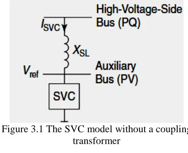
SVC Operation within the Control Range: If the slope of the SVC is neglected, then the SVC is modeled as a PV bus, with P =0 and V =Vref. However, if the slope is considered (as in the analysis of weak ac systems), the same is modeled by connecting the high-voltage side of the SVC bus to a fictitious auxiliary bus by means of a reactance

equal to the slope expressed in per units on the SVC base. Such a model is shown in Figure 3.1.

Figure 3.1 The SVC model without a coupling transformer

4. THYRISTOR CONTROLLED SERIES CAPACITOR (TCSC)

A TCSC involves continuous-time dynamics, relating to voltages and currents in the capacitor and reactor, and nonlinear, discrete switching behavior of thyristors. Deriving an appropriate model for such a controller is an intricate task.

Variable-Reactance Model:

A TCSC model for transient- and oscillatory-stability studies, used widely for its simplicity, is the variable-reactance model. In this quasi-static approximation model, the TCSC dynamics during power-swing frequencies are modeled by a variable reactance at fundamental frequency. The other dynamics of the TCSC model—the variation of the TCSC response with different firing angle. It is assumed that the transmission system operates in a sinusoidal steady state, with the only dynamics associated with generators and PSS. This assumption is valid, because the line dynamics are much faster than the generator dynamics in the frequency range of 0.1–2 Hz that are associated with angular stability studies. In the variable-reactance model for stability studies, a reference value of TCSC reactance, Xref, is generated from a power-scheduling controller based on the power-flow specification in the transmission line. The reference Xref value may also be set directly by manual control in response to an order from an energy-control center, and it essentially represents the initial operating point of the TCSC; it does not include the reactance of FCs (if any). The reference value is modified by an additional input, Xmod, from a modulation controller for such purposes as damping enhancement. Another input signal, this applied at the summing junction, is the open-loop

SYSTEM SYSTEM G L GG LG GL LL G L

SYSTEM

Y

V

V

V

Y

Y

Y

Y

I

I

I

_

=

auxiliary signal, Xaux, which can be obtained from an external power-flow controller. A desired magnitude of TCSC reactance, Xdes, is obtained that is implemented after a finite delay caused by the firing controls and the natural response of the TCSC. This delay is modeled by a lag circuit having a time constant of typically 15–20 ms. The output of the lag block is subject to variable limits based on the TCSC reactance-capability curve .The resulting XTCSC is added to the Xfixed, which is the

reactance of the TCSC installation’s FC component. To obtain per-unit values, the TCSC reactance is divided by the TCSC base reactance, Zbase, given as

--- (4.1)

The TCSC model assigns a positive value to the capacitive reactance, so Xtotal is multiplied by a

negative sign to ensure consistency with the convention used in load-flow and stability studies. The TCSC initial operating point, Xref, for the

stability studies is chosen as

---- (4.2) 5. RESULTS AND ANALYSIS

In order to analyse, a standard IEEE 5-Bus test system is considered as shown below.

Figure 5.1 IEEE-5 Bus test system

Case 1: Under Steady State Condition

Load Flow Programme is executed in MATLAB using Newton - Raphson method under steady state condition. A weak bus is identified by using L-Index method, which indicates the stability condition of the system. The bus with a weak voltage profile is incorporated with FACTS. These FACTS are optimally placed based on the L-index value, i.e. the index with the highest value indicates as an optimal location to enhance the voltage stability.

5.1 Without FACTS

Initially load flows are executed under normal condition without FACTS and a weak bus is identified as Bus-5 with a least voltage magnitude i.e., 0.9776 (p.u) as shown in Table 5.1, in which column1 represents Bus No.,column2 represents Voltage Magnitudes in (p.u) and column3 represents PhaseAngles in (Degrees).

The stability condition of the system is identified using L-Index method as shown in Table 5.2 in which, column 1 represents BusNo. and column 2 represents L-Index value . The L-Index value of Bus -5 is the highest value and its corresponding voltage magnitude is least value from all Buses.Therefore bus-5 can be identified as a weak Bus and it reaches to Instability.

Table 5.1 Bus Voltage Magnitudes and Phase Angles without FACTS under steady state Condition

Table 5.2 L-Indices without FACTS under steady state Condition

Bus No.

L-Index without FACTS

3 0.0299

4 0.0304

5 0.0328

5.2 With SVC

Table 5.3 : Bus Voltage Magnitudes and phase angles after the placement of SVC under steady

state Condition

Table 5.4: L-indices with SVC under steady state Condition

Bus No.

Voltage Magnitudes

(p.u)

PhaseAn gle

(Degrees

1 1.0600 0

2 1.0000 -2.0574

3 0.9925 -4.7163

4 0.9894 -5.0340

5 0.9776 -5.8490

Bus No.

Voltage Magnitudes

(p.u)

PhaseAn gle

(Degrees)

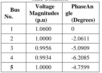
1 1.0600 0

2 1.0000 -2.0611

3 0.9956 -5.0909

4 0.9934 -6.2085

By incorporating SVC at Bus-5, load flows are executed under normal condition and voltage magnitude at bus-5 is improved from 0.9776(p.u) to 1.000 (p.u.) as shown in Table 5.3, in which column1 represents BusNo.,column2 representsVoltage Magnitudes in (p.u.) and column3 represents PhaseAngles .

The stability condition of the system is identified using L-Index method as shown in Table 5.4 in which, column -1 represents BusNo. and column -2 represents L-Index value . After the placement of SVC ,the L-Index value of Bus -5 is reduced to 0.0099 and its corresponding voltage magnitude is improved .

The L-Index values of buses with and without SVC are summarized as shown in Table 5.5 and it is reduced to 0.0099 p.u. after placing SVC at Bus -5.

Table 5.5 L-Indices Without And With SVC Under Steady State Condition

Bus No.

L-index without SVC

L-index

with SVC

3 0.0299 0.0262

4 0.0304 0.0267

5 0.0328 0.0099

5.3 With TCSC

Table 5.6: Bus Voltage Magnitudes And Phase Angles With TCSC Under Steady State Condition

By incorporating TCSC in series with the transmission line between Bus-4 and Bus-5, load flows are executed under normal condition and the voltage magnitude at bus-5 is improved from 0.9776(p.u) to 0.9789 (p.u.) as shown in Table 5.6, in which column1 represents Bus No.,column2 represents Voltage Magnitudes in (p.u) and column3 represents PhaseAngles in (Degrees).Due to the incorporation of TCSC in series with the transmission line an extra node will appear and it is taken as Bus No.6.

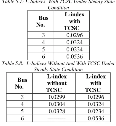
The stability condition of the system is identified using L-Index method as shown in Table 5.7. in which, column 1 represents BusNo. and column 2 represents L-Index value . After the placement of TCSC ,the L-Index value of Bus -5 is reduced to 0.0234 and its corresponding voltage magnitude is also improved.

Table 5.7: L-Indices With TCSC Under Steady State Condition

Bus No.

L-index with TCSC

3 0.0296

4 0.0324

5 0.0234

6 0.0536

Table 5.8: L-Indices Without And With TCSC Under Steady State Condition

Bus No.

L-index without TCSC

L-index with TCSC

3 0.0299 0.0296

4 0.0304 0.0324

5 0.0328 0.0234

6 --- 0.0536

Case 2 : Fault Condition

After analysing the Voltage Stability under Normal Condition then by changing the Reactive Power at bus-5, keeping the Real and Reactive Powers at all other Buses remain fixed, the instability point is identified using L-Index method and corresponding Bus with a weak Voltage Profile is improved . The enhancement of voltage is carried out through the optimal placement of SVC and TCSC. The Optimal location is identified by selecting a weak voltage profile..When the reactive power is increasing at bus -5, the voltage magnitude at that bus is gradually decreasing and its corresponding L-Index value is increasing as shown in Table 5.9.

Bus No.

L-index with SVC

3 0.0262

4 0.0267

5 0.0099

Bus No.

Voltage Magnitudes

(p.u.)

Phase Angles

(Degrees)

1 1.0600 0

2 1.0000 -1.5604

3 0.9966 -3.5114

4 0.9924 -4.0915

5 0.9789 -5.1822

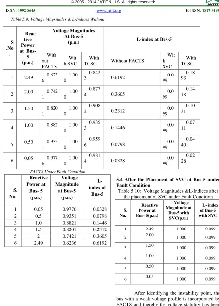
Table 5.9: Voltage Magnitudes & L-Indices Without

FACTS Under Fault Condition

S. No.

Reactive Power at

Bus- 5 (p.u.)

Voltage Magnitude

at Bus-5 (p.u.)

L- index of

Bus-5

1 0.05 0.9776 0.0328

2 0.5 0.9351 0.0798

3 1.0 0.8821 0.1446

4 1.5 0.8201 0.2312

5 2 0.7421 0.3605

6 2.49 0.6236 0.6192

5.4 After the Placement of SVC at Bus-5 under Fault Condition

Table 5.10: Voltage Magnitudes &L-Indices after the placement of SVC under Fault Condition

S. No.

Reactive Power at Bus- 5(p.u.)

Voltage Magnitude at

Bus-5 with SVC(p.u.)

L- index of Bus-5 with SVC

1 2.49 1.000 0.099

2 2.00 1.000 0.099

3 1.50 1.000 0.099

4 1.00 1.000 0.099

5 0.50 1.000 0.099

6 0.05 1.000 0.099

After identifying the instability point, the bus with a weak voltage profile is incorporated by FACTS and thereby the voltage stability has been enhanced under transient conditions as shown in Table 5.10, in which column 1 represents reactive power at load Bus 5, column2 represents Voltage Magnitude at Bus 5 in (p.u.) and column 3 represents L-Index values after the placement of S

.No .

Reac tive Power at Bus-5 (p.u.)

Voltage Magnitudes At Bus-5

(p.u.) L-index at Bus-5

With out FACTS

Wit h SVC

With

TCSC Without FACTS

Wit h SVC

With TCSC

1 2.49 0.623

6

1.00 0

0.842

3 0.6192 0.0

99

0.18 93

2 2.00 0.742

1

1.00 0

0.877

4 0.3605 0.0

99

0.14 18

3 1.50 0.820

1

1.00 0

0.908

2 0.2312 0.0

99

0.10 31

4 1.00 0.882

1

1.00 0

0.935

3 0.1446 0.0

99

0.07 11

5 0.50 0.935

1

1.00 0

0.959

6 0.0798 0.0

99

0.04 40

6 0.05 0.977

6

1.00 0

0.981

4 0.0328 0.0

99

SVC. These are performed at different Reactive powers at Bus5.

5.5 After the Placement of TCSC under Fault Condition

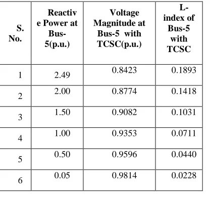
Due to the optimal placement of TCSC in series with the Transmission Line between Bus 4 and Bus5, the Voltage Profile at Bus5 is improved under Transient conditions at different Load Reactive Powers as shown in Table 5.11. L-Indiex values are also determined at each condition.

From the analysis of results due to change in load reactive powers at Bus5, voltage magnitudes are gradually decreasing from their nominal values . if the reactive power at load bus 5 increases further from 2.49 p.u. then the voltage magnitudes are drastically reduced and almost all the syatem is going to collapse.

Due to the gradual change in Load Reactive Power at Bus5 in different steps ,the system voltage magnitudes are gradually decrease and the instability point is obtained at Load Reactive Power 2.49 p.u. . This instability point is estimated through the determenation of L-Index value.

Table 5.11: Voltage Magnitudes & L-Indices after the placement of TCSC under Transient Condition

S. No.

Reactiv e Power at

Bus- 5(p.u.)

Voltage Magnitude at

Bus-5 with TCSC(p.u.)

L- index of

Bus-5 with TCSC

1 2.49 0.8423 0.1893

2 2.00 0.8774 0.1418

3 1.50 0.9082 0.1031

4 1.00 0.9353 0.0711

5 0.50 0.9596 0.0440

6 0.05 0.9814 0.0228

5.5 Summary of Results

Table 5.12: Voltage Magnitudes and L-Indices of Bus5 Without and With FACTS under Fault

Condition

The system stability is then enhanced through the optimal placement of FACTS such as SVC and TCSC using L-Index method . After the incorporation of FACTS , the voltage magnitudes are increased and the L-Index value is decreased at

different Load Reactive Powers and are listed as shown in Table 5.12.

6. CONCLUSION:

From these results , it is obsereved that , due to the incorporation of SVC, the Voltage Magnitudes are improved much better than TCSC and L-Index values are reduced. Hence SVC is better than TCSC while the enhancement of voltage stability at different Reactive powers and are listed in Table 5.12. This can be achieved by adjusting the sapecifications of FACTS while performing the load flows with the help of MATLAB.

REFERENCES:

[1] Kundur.P, 1994, “Power System Stability and Control”. New York: Tata McGraw-Hill. [2] Kiran Kumar. kuthadi “Enhancement of

Voltage Stability through Optimal Placement of FACTS Controllers in Power Systems” American Journal of Sustainable Cities and Society, Issue- 1 , Vol -1 July 2012. [3] N. G. Hingorani “Power Electronics in

Electrical Utilities: Role of Power Electronics in Future Power Systems,” Proceedings of the IEEE, Vol.76 No.4, Pp.481-482, Apr.1988.

[4] G. W. Stagg. and A. H. El-Abiad, “Computer Methods inPower System Analysis”, McGraw-Hill, 1968

[5] I.Kumarswamy and P. Ramanareddy,“Analysis of Voltage Stability Using L-Index Method” April 2011 : Copyright @2011, ECO Services International.

[6] Enrique Acha “FACTS modeling and simulation in power networks” University of Glasgow, UK.

[7] S. B. Bhaladhare , P.P. Bedekar “ Enhancement of Voltage Stability through Optimal Location of SVC ” International Journal of Electronics and Computer Science Engineering, ISSN-2277-1956/V2N2- 671-677.

[8] Mohammed Osman Hassan, S. J. Cheng “Steady-State Modeling of SVC and TCSC for Power Flow Analysis”, Proceedings of the International Multi Conference of Engineers and Computer Scientists 2009, Vol -2-IMECS 2009, March 18 - 20, 2009.

analysis”, Int.J. Power Energy Syst., 17(1), pp. 28-37.

[10] Carson, W., Taylor, 1994, “Power System Voltage Stability”, Tata- McGraw Hill. Third Edition.

[11] Dong.F., Chowdhury.B.H., Crow.M.L. and Acar.L., 2005, “Improving voltage stability by reactive power reserve management,” IEEE Trans.Power Syst., vol. 20(1), pp. 338– 345.

[12] Mohamed, A., 1994, “New Techniques for Power System Voltage Stability Studies”, University of Malaya, Malaysia, 1994. [13] Mohamed, A. and Jasmon, G. B., 1991, “A

New Clustering Technique for Power System Voltage Stability Analysis”, Journal of Electric Machines and Power Systems, 23, pp. 389-403.

[14] VanCutsem,T. and Vournas.C.D., 1998, “Voltage Stability of Electric Power Systems” . Norwell, MA: Kluwer.