International Journal of Emerging Technology and Advanced Engineering
Website: www.ijetae.com (ISSN 2250-2459, ISO 9001:2008 Certified Journal, Volume 7, Issue 12, December 2017)
125
Time Series Forecasting Using Fuzzy Time Series With Hedge
Algebras Approach
Minh Loc Vu
1, The Yen Pham
2, Thanh Nghia Huynh Pham
31,2
Faculty of Computer, Gia Dinh University, Vietnam 3
Faculty of Basic Sciences, Baria-Vungtau University, Vietnam
Abstract— During the recent years, many different methods of using fuzzy time series for forecasting have been published. This paper presents a novel technique based on the hedge algebras (HA) approach. Based upon the HA, the fuzziness intervals are used to quantify the values of fuzzy time series. The intervals are determined through the fuzziness intervals and the adjusted fuzzy logical relationships. The experimental results, forecasting enrolments at the University of Alabama, demonstrate that the proposed method significantly outperforms the published ones.
Keywords—Forecasting, Fuzzy time series, Hedge algebras, Enrolments, Intervals.
I. INTRODUCTION
Fuzzy time series was originally proposed by Song and Chissom[1] and it has been applied to forecast the enrolments at University of Alabama [2, 3]. All steps in the procedure of using fuzzy time series to forecast time series fall into three phases, Phase 1: fuzzifying historical values, Phase 2: mining the fuzzy logical relationships, Phase 3: defuzzifying the output to get the forecasting values. In 1996, Chen [4] opened a new study direction of using fuzzy time series to forecast time series. In this study, Chen suggested an idea of utilizing the intervals in the formula of computing the forecasting values by only using the arithmetic operators. Since then, clearly, it seems to be that Phase 1 strongly affects the forecasting accuracy rate. We can see that the step of partitioning the universe of discourse belongs to Phase1.
Partitioning the universe of discourse is the essential issue in the method of using fuzzy time series as a tool for forecasting time series. Indeed, product of partitioning the universe of discourse is the intervals as the source that provides the values in the future of time series. So, the better method to partition the universe of discourse we have, the better forecasting values we get. Commonly, the method of partitioning the universe of discourse can be divided into two types through the resulted intervals, equal or not the sized intervals.
From the empirical results in the list, applying the second type gives the better forecasting accuracy rate than others. Thus, recent researches focus on the second method. There have been many methods of partitioning the universe of discourse such as [5] which is the first research confirmed the important role of partitioning the universe of discourse, this employed distribution and average based length as a way to solve the problem. In turn, Jilani et al. [6] proposed frequency density, Huarng and Yu [7] suggested the ratios and Bas et al. [8] used modified genetic algorithm as basis to improve quality of intervals. Information granules were applied in [9, 10, 11] to get good intervals on the universe of discourse. By the hedge algebras approach Ho et al. [12] presented a method of partitioning the universe of discourse. According to this approach, fuzziness intervals are used to quantify the values of fuzzy time series that are linguistic terms. These fuzziness intervals are employed as intervals on the universe of discourse.
Based upon the fuzziness intervals of values of fuzzy time series, distribution of historical values of time series and adjusted fuzzy logical relationships, we can get the intervals on the universe of discourse. This is the way that the proposed method works.
The rest of this paper is organized as follows: Section 2 briefly introduces some basis concepts of HA; Section 3 presents the proposed method; Section 4 presents empirical results on forecasting enrollments at University of Alabama, Forecasting TAIEX Index and comment; Section 5 concludes the paper.
II. PRELIMINARIES
In this section, we briefly recall some concepts associated with fuzzy time series and hedge algebras.
A. Fuzzy time series
International Journal of Emerging Technology and Advanced Engineering
Website: www.ijetae.com (ISSN 2250-2459, ISO 9001:2008 Certified Journal, Volume 7, Issue 12, December 2017)
126
It can be seen that conventional time series are quantitative view about a random variable because they are the collection of real numbers. In contrast to this, as the collection of linguistic terms, fuzzy time series are qualitative view about a random variable. There are two types of fuzzy time series, time-invariant and time-variant fuzzy time series. Because of practicality, the former is the main subject which many of researchers focus on. In most of literature, the linguistic terms are quantified by fuzzy sets. Formally, fuzzy time series are defined as following definitionDefinition 1. LetY
(
t
)
(t
=
...,
0,1,2,...), a subset of R1,
be the universe of discourse on which fi(
t) (i = 1,2,...) are defined and F(t) is the collection of fi(
t) (i = 1,2,...). Then F(t) is called fuzzy time series on Y(
t
)
(t
=
...,
0
,
1
,
2
,...)
.Song and Chissom employed fuzzy relational equations as model of fuzzy time series. Specifically, we have following definition:
Definition 2.If for any
f
j(
t
)
∈
F
(
t
), there exists anf
i(
t-
1)
∈
F
(
t-
1)
such that there exists a fuzzy relationR
ij(
t,t
-1)
andf
j(
t
) =
f
i(
t
-1)
∘R
ij(
t,t
-1)
where “∘” is the max-min composition, then F(t) is said to be caused by F(t-1) only.Denote this as
f
i(
t-
1) →
f
j(
t
)
or equivalently
F
(
t-
1) →
F
(
t
)
In [2, 3], Song and Chissom proposed the method which use fuzzy time series to forecast time series. Based upon their works, there are many studies focus on this field.
B. Some basis concepts of Hedge Algebras
In this section, we briefly introduce some basis concepts in HA, these concepts are employed as basis to build our proposed method. HA are created by Ho Cat Nguyen et al. in 1990. This theory is a new approach to quantify the linguistic terms differing from the fuzzy set approach. The HA denoted by AX = (X,G,C,H,≤ ), where,
G = {c+,c−} is the set of primary generators, in which c+
and c− are, respectively, the negative primary term and the positive one of a linguistic variable X, C = {0,1,w} a set of constants, which are distinguished with elements in X,H is the set of hedges, “≤” is a semantically ordering relation on X.
For each x ∈ X in HA, H(x) is the set of hedge u ∈ X that generated from x by applying the hedges of H and denoted u = hn,...,h1 x, with hn,...,h1 ∈ H. H = H
+ ∪
H−, in which H− is the set of all negative hedges and H+ is the set of all positive ones of X. The positive hedges increase semantic tendency and vice versa with negative hedges. Without loss of generality, it can be assumed that.
H
−= {
h
−1< h
−2<
···
< h
−q}
andH
+= {
h
1< h
2<
···
<
h
p}.
If X and H are linearly ordered sets
,
then AX = (X,G,C,H,≤ ) is called linear hedge algebra, furthermore, if AX is equipped with additional operations Σ and Φ that are, respectively, the infimum and supremum of H(x), then it is called complete linear hedge algebra (ClinHA) and denoted AX = (X,G,C,H,Σ,Φ,≤)
.
Fuzziness of vague terms and fuzziness intervals are two concepts that are difficult to define. However, HA can reasonably define these ones. Concretely, elements of H(x) still express a certain meaning stemming from x, so we can interpret the set H(x) as a model of the fuzziness of the term x. With fuzziness intervals can be formally defined by following definition.
Definition 3. Let AX = (X, G, C, H, ) be a ClinHA
.
Anfm
:
X
[0,1]
is said to be a fuzziness interval of terms in X if:
(1).
fm
(
c
)
+fm
(
c
+)
=
1
and ( ) ( )h H fm hu fm u
,
for
u
X
;
in this casefm
is called complete;
(2
). For the constants 0, W and 1,
fm
(
0
)
= fm
(
W
)
=
fm
(
1
)
=
0;
(3). For x, yX,h H, ( ) ( )
( ) ( )
fm hx fm hy fm x fm y
, that is this
proportion does not depend on specific elements and, hence, it is called fuzziness measure of the hedge h and denoted by (h).
Proposition 3
.
For each fuzziness intervalfm
on X the following statements hold:(1)
.
fm
(
hx
) =
(
h
)
fm
(
x
),
for every x
X
;
(2)
.
fm
(
c
)
+
fm
(
c
+) = 1;
(3). ( ) ( )
0
,i fm hc fm c p
i
q i
,
c
{
c
International Journal of Emerging Technology and Advanced Engineering
Website: www.ijetae.com (ISSN 2250-2459, ISO 9001:2008 Certified Journal, Volume 7, Issue 12, December 2017)
127
(4). ( ) ( )
0
,i fm hx fm x p
i
q i
;
(5).
q i 1 (hi)
and
1ip(hi),
where
,
> 0
and
+
= 1.
HA build the method of quantifying the semantic of linguistic terms based on the fuzziness intervals and hedges through mapping that fit to the conditions in following definition.
Definition 4. Let AX = (X, G, C, H, , , ) be a CLinHA. A mapping : X [0,1] is said to be an semantically quantifying mapping of AX, provided that the following conditions hold:
(1). is a one-to-one mapping from X into [0,1] and preserves the order on X, i.e. for all x, yX, x < y
(x) < (y) and (0) = 0, (1) = 1, where 0, 1 C;
(2). Continuity: x X, (x) = infimum (H(x)) and (x) = supremum(H(x)).
Semantically quantifying mapping is determined concretely as follows.
Definition 5. Let fm be a fuzziness interval on X. A mapping : X [0,1], which is induced by fm on X, is defined as follows:
(1). (W) = = fm(c), (c) = − fm(c) = fm(c), (c+)=+ fm(c+);
(2). (hjx) = (x) +
j j Sign
i i j j
j
x
fm
h
x
h
x
fm
h
x
h
Sign
) ((
)
(
)
(
)}
){
(
,where j {j: qjp & j0} = [-q^p] and
(hjx) [1 ( ) ( )( )] { , }
2
1
Sign hjx Sign hphjx ;
(3). (c) = 0, (c) = = (c+), (c+) = 1,and for j
[q^p] ,
(hjx) = (x) + Sign(hjx)
) ( ) (
(
)
(
)}
{
ijsignsignjj
h
ifm
x
2
1
(1Sign(hjx))(hj)fm(x),
(hjx)=(x) + Sign(hjx)
) ( ) (
(
)
(
)}
{
j signjj sign
i
h
ifm
x
+2
1
(1+Sign(hjx))(hj)fm(x).
The Sign function is determined in the following
Definition 6. A function Sign: X {1, 0, 1} is a mapping which is defined recursively as follows, for h, h'H and c
{c, c+}:
(1). Sign(c) = 1, Sign(c+) = +1;
(2). Sign(hc) = Sign(c), if h is negative w.r.t. c;
Sign(hc) = + Sign(c), if h is positive w.r.t.c;
(3). Sign(h'hx) = Sign(hx), if h’hx hx and h' is negative w.r.t. h;
Sign(h'hx) = + Sign(hx), if h’hx hx and h' is positive w.r.t. h.
(4). Sign(h'hx) = 0 if h’hx = hx.
Definition 7. [12] Given
AX
2,
(
k
1
)
, the similar fuzzyspace of set
X
(k)denoted
(k) is a set of similar fuzzyspace of all grades from
X
(k) for
x
X
(k),
g(x)k
x
l
g
k
(),
(
)
unchanged ( ie
x
X
(k),
g(x) madeup of the same fuzzy space of level
k
*) and
(k) is apartition of [0,1].
Definition 8. [12] Given
AX
2,
k
1
,
x
X
(k)identify the similar fuzzy spaceg(x)
(k)definition ofthe compatibility level
g
k
2
l
(
x
)
of quantitative value
for Gradex
to be a mapping]
1
,
0
[
]
1
,
0
[
:
X
s
g determined based on the distancefrom
to
(x
)
and two similar fuzzy space close tog(x) as follows:
,
0
)
(
)
(
)
(
,
)
(
)
(
)
(
min
max
)
,
(
x
z
v
x
y
x
x
v
x
v
s
g
Where y, z are two grades defining two similar fuzzy space neighbors left and right of g(x).
International Journal of Emerging Technology and Advanced Engineering
Website: www.ijetae.com (ISSN 2250-2459, ISO 9001:2008 Certified Journal, Volume 7, Issue 12, December 2017)
128
III. THE PROPOSED METHODFor convenience to present proposed method, we name the linguistic values of fuzzy time series as the variables Ai
with i ∈N. Revυ(x) and Rev fm(x) are the reversed mapping
of υ(x) and fm(x), respectively, from [0,1] to the universe of
discourse of fuzzy time series U. Denote Ik, on U, is the
interval corresponding to Ak.
A. Rule for adjusting the fuzzy logical relationships
We can adjust the fuzzy logical relationships to improve forecasting result depending upon the concrete forecasting problem. The rule for adjusting is as follows
Consider sequentially for each group of fuzzy logical relationships. With the group of fuzzy logical relationships considered such as Ai → Aj,...,Ai → Ak,..., and if |j − k| ≥ 1
then.
If (j < k) then replacing Ak or Aj do not affect any next
fuzzy logical relationships, then
If the historical value called aj in fuzziness interval of
Aj, Ij, and |Rev υ(Aj)−aj |> |Rev υ(Aj+1) − aj|, then extend Ij+1 to cover up aj. (r.1)
If the historical value called bk in fuzziness interval of Ak,Ik, and |Rev υ(Ak−1)− bk| < |Rev υ(Ak) − bk|, then extend
Ik−1 to cover up bk. (r.2)
Do the same with the case of j > k.
Aj and Ak are as close as possible that is the goal we
would like to reach up. We can do (r.1) or (r.2) because the following reason:
With Am is the linguistic term that we are considering. If Revυ(Am) is the semantically quantifying mapping of Am
on the universe of discourse, then one also is the semantic core of Am. If the other values belonging to the fuzziness
interval of Am, then they are semantically equal to Revυ(Am), that means they together reflex the meaning of
Am. If a is the value that belong to Am(+1) and |Revυ(Am)−a|
> |RevυA(m+)1−a|, then a is more close semantic with Am+1 than Am. So, we can extend fm(Am+1) to cover up a
B. Method for partitioning the universe of discourse
The proposed method, named VML, is described as follows
Step 1:
Determine the U, the universe of discourse of fuzzy time series F(t).
U = [min(F(t))−D1,max(F(t))+D2], where D1 and D2 are proper positive numbers.
Set n is the number of intervals that we would like to divide on the universe of discourse.
Step 2:
Building the ClinHA with only two hedges, h−1 and h+1,
AX = (X,G,H,Σ,Φ,≤ ) corresponding to linguistic variable
that is considered as fuzzy time series F(t). That means determining the set of parameters of AX model needs to be consistent with the context of the problem “forecasting student enrolment number at the Alabama University”.
According to the definitions and propositions in Section II.B, parameters of the ClinHA, which contain two hedges,
h−1 and h+1, have the following properties
µ(h+1) = β = fm(c+); µ(h−1) = α = fm(c−) where α,β > 0,
α + β=1.And υ(W) = fm(c−) = θ υ(c−) = βfm(c−); υ(c+) = 1
− βfm(c−) where 0,W,1 are constants and
fm(0) = fm(1) = fm(W)=0 ; υ(W) = θ = W.
By having knowledge of W and µ(h+1) or µ(h11), other parameters can be determined. Now let us define two parameters W and µ(h) that fit the context of the problem based on the historical values and exploit the relationship between them: According to the context, semantics of (t) denotes number of the enrollment students at the medium level and W is the normalization value of , they are calculated according formulas:
where xi is the historical value of F(t), e.g. x1 =
F(1971),...,x22 = F(1992).
The value difference between two adjacent historical values will be the basis for forecasting time series: At time t, it will forecast the trend to increase if the previous historical value is smaller than it, otherwise forecasting trend decreases. In the general case, the average value of the difference will be the basis for forecasting which is defined by the following equation
To have a better forecasting, we continue to exploit the data relation of historical values based on the relationship between S¯ with two values to characterize the increment or decrement of forecasting at maximum difference values
for 1 ≤ i ≤ n − 1 (4)
(1)
(2)
International Journal of Emerging Technology and Advanced Engineering
Website: www.ijetae.com (ISSN 2250-2459, ISO 9001:2008 Certified Journal, Volume 7, Issue 12, December 2017)
129
for 1 ≤ i ≤ n − 1 (5)Clearly,
Let
If S+ ≥ S− then h := h+1 else h := h−1.
There is an induced about the trend change in the forecasting in the discourse space into the space of [0, 1] where there is a trend change to the quantitative semantics value due to the impact on the terms of the hedges. That is the basic to we construct the mathematics model for forecasting time series by (HA) approach. Until now, I have finished to construct the ClinHA with only two hedges by method of define two parameters W and µ(h) based on analyzing data of forecasting.
In this paper, I build AX = (X,G,H,Σ,Φ,≤) as follows:
Let G={C−=Low(Lo), C+ = High(Hi)} and
H = H+ ∪ H−.
H− = {Litlle(L)} and H+ = {Verry(V)}. Calculate W using (1) and (2).
Calculate µ(h+1) or µ(h−1) using (3), (4) and (5).
Calculate the remaining parameters according to Section II.B.
Using above HA generate n linguistic terms which use to qualitatively describe time series. The way to determine these linguistic terms as follows: Applying two hedges, h−1 and h+1, on the primary generators c− and c+, from left to right to generate the linguistic terms.
If the number of linguistic terms are less than, one interval, the number of intervals that we need to divide, then find the interval that contain maximum amount of historical values, assuming that this interval corresponding to the linguistic term Ai. From Ai generating two linguistic
term h−1Ai and h+1Ai.
Step 3: Based upon the distribution of historical values, put them into the corresponding linguistic term fuzziness interval.
C. Forecasting Algorithm
Step 1:
Apply VML to partition the universe of discourse.
Step 2:
Mine the fuzzy logical relationships: Ap → Aq, where Ap
and Aq, respectively, are the linguistic values of F(t) and F(t + 1) respectively.
Set the group of fuzzy logical relationships having the same left side: At → Au(m)···Av(n), m,··· ,n are the number
of iterations of fuzzy logical relationship At → Au and At → Av.
Adjust the fuzzy logical relationships following rule III.A.
Step 3: Suppose that the time series value at (t − l), ft,
belongs to Revfm(At) then
(t) =
Rev A
u···
Rev A
(
v)
l
(6)
where (t) is the forecasting value at time t and
l = card{u,··· ,v}.
IV. RESULT AND COMMENT
The proposed approach is applied to forecast the enrolments at the University of Alabama from year 1971 to 1992 (n = 22). The result will then be compared with different published methods. To measure the accuracy of the forecasting methods, the following metrics are used for comparison.
The Root-Mean-Square-Error (RMSE) which is defined as
RMSE=
2
1
(
)
n
i i i
X
X
n
The Numerical Error (NE) percentage
NE(%) =
1
(
)
1
|
| 100
n i i
i
i
X
X
n
X
The Normalized Numerical Error (NNE) percentage
NNE(%) = 1
( )
1
| | 100
max( ) min( )
n i i
i
X X
n x x
International Journal of Emerging Technology and Advanced Engineering
Website: www.ijetae.com (ISSN 2250-2459, ISO 9001:2008 Certified Journal, Volume 7, Issue 12, December 2017)
130
where i are the forecasted value and the actual value attime i respectively, and n is the length of the time series to be forecasted.
A. Result
We apply proposed method for the intervals of 7 and 17.
Interval 7
Apply the VML method to partition the universe of discourse
max(F(t)) = 20000 min(F(t)) =13000
Follow (1-3.2) and (2-3.2) we
have
According to (3-3.2),(4-3.2) and (5-3.2),
S¯ = 510S+ = |x18 − x17| = |18150 − 16859| = 1291 S− = |x12 − x11| = |15433 − 16388| = 955
As S+ > S− , according to (6-3.2), µ(V ) = W = 0.4563 hence, fm(V.Lw) = υ(Lw) =0.20821
Based on the distribution of historical values we can put the historical values into the following intervals
A1 = [0,υ(VVV,Lw),υ(Lw)] where 0 and υ(Lw) are the left and right border of the linguistic values “LLV.Lw” respectively. “LVV.Lw” stands for “Little-Very-Very-Low”. Similarly,
A2 = [υ(Lw),υ(L.Lw),υ(LVL.Lw)]
A3 = [υ(LVL.Lw),υ(VL.Lw),υ(VVL.Lw)]
A4 = [υ(VVL.Lw),υ(VL.Hi),υ(LLVL.Hi)]
A5 = [υ(LLVL.Hi),υ(L.Hi),υ(LL.Hi)]
A6 = [υ(LL.Hi),υ(VLL.Hi),υ(Hi)]
A7 = [υ(Hi),υ(V.Hi)] The values of calculated Ii are
The semantically quatifying mappings can also be obtained
Rev(A1) = 13303 Rev(A2) =15402 Rev(A3) = 15833 Rev(A4) =16625 Rev(A5) = 17138 Rev(A6) =17795 Rev(A7) = 19207
Table I :
Historical and fuzzified values
Years Enrollments Fuzzified Values
1971 13055 A1
1972 13563 A1
1973 13867 A1
1974 14696 A2
1975 15460 A2
1976 15311 A2
1977 15603 A3
1978 15861 A3
1979 16807 A5
1980 16919 A5
1981 16388 A4
1982 15433 A2
1983 15497 A2
1984 15145 A2
1985 15163 A2
1986 15984 A3
1987 16859 A5
1988 18150 A6
1989 18970 A7
1990 19328 A7
1991 19337 A7
International Journal of Emerging Technology and Advanced Engineering
Website: www.ijetae.com (ISSN 2250-2459, ISO 9001:2008 Certified Journal, Volume 7, Issue 12, December 2017)
131
Table II:Group of fuzzy logical relationships
Group 1 A1A1 (2), A1A2
Group 2 A2A2 (5), A2→A3(2)
Group 3 A3A3, A3A5 (2)
Group 4 A4A2
Group 5 A5A4, A5A5, A5A6
Group 6 A6A7
Group 7 A7A7(3)
Comments
We compare our approach with the method Wei Lu et.al. published in [11] to illustrate our superior efficiency. After commenting on the research publication of other authors, Wei Lu confirmed As noted above, the objective of our research is to develop a novel method of partitioning the universe of discourse deliver some remedy for these shortcoming [11].
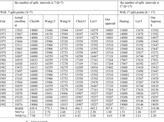
Table III: Sum up Compare Forecasting Result of Methods (with h=7 and h=17).
Our comparison focuses on two aspects: the calculation convenience and the forecasting accuracy.
First, the convenience in calculations: only with the simple calculations using Method for partitioning the universe of discourse and Algorithm for forecasting”, we have obtained results about group of logical relationship like the results from Wei Lu [11]. However, our calculation is much simpler than theirs as shown in Table II.
Second, the forecasting accuracy: Table 3 shows our proposed method is about 10% better in term of accuracy (all metrics) compared to Wei Lu et.al. approach [11].
The reason is because Wei Lu et.al. chose middle point of interval to defuzzifying the forecasting outputs [11] as the basis to calculate the forecasting results hence it carried heavy subjective and is not related to the inherent semantic of information granules (as linguistic values). While with our approach, similarity fuzziness interval (for semantics) is used to fuzzifying the historical data of time series and its quantitative semantic value (as the its semantic core) is the basis for the forecasting.
These values are calculated by determining two parameters using Method for partitioning the universe of discourse mentioned above. It is not decisive subjective and contrast in accordance with the context of forecasting problems, because Hedge algebras are considered as an algebraic approach to the inherent word semantics and word-domains of each individual linguistic variable, which is simply understood as a variable whose values are definite linguistic words of a natural language and establish a formalized foundation to develop quantitative semantics of words, including their fuzzy set based semantics [15]. If Adjusting the fuzzy logical relationships according to Rule III.A mentioned above:
A2 → A3, the historical values of I2 are 14696, 15145, 15163, 15311, 15433, 15460, 15497 and with I3 are 15603, 15861, 15984. Revυ(A2) = 15402, Revυ(A3) = 15833.
|15402 − 15603| = 201 < |15833 − 15603| = 230,
hence I2 = [14457,15604) and I3 = [15604,16029) and
A2 → A3 replaced by A2 → A2.
Then the result is even more accurate as RMSE = 387.4, NE(%) = 1.80% and NNE(%) = 4.63%.
This proves Step 2. Find the optimal split point vector S
= p1,p2,.pi..,ph-1ph in the universe of discourse U [11], which be the step is core of our approach[11] has not yet reached optimal.
It is important that in a natural language, semantics of linguistic words be decisive by context. Consequently, That means determining the set of parameters of AX model needs to be consistent with the context of problem of the forecasting student enrollment number at the Alabama University mentioned above, it is interpretation for self-affirmed superior efficiency of our approach
B. Interval of 17
Similarly, apply the proposed method for 17 intervals on the universe of discourse we will have the forecasting result as:
RMSE = 216.1; NE = 0.97%; NNE = 2.20%
Table III. shows that all the metrics: RMSE, NE(%) and NNE(%) of our proposed method is less than of the others
International Journal of Emerging Technology and Advanced Engineering
Website: www.ijetae.com (ISSN 2250-2459, ISO 9001:2008 Certified Journal, Volume 7, Issue 12, December 2017)
[image:8.612.50.578.166.560.2]132
Table IIISum up Compare Forecasting Result of Methods with h=7 and h=17.
V. CONCLUSION
In this paper we presented the proposed method using fuzzy time series with HA approach to forecast enrolments at the University of Alabama. Whereby, based upon the number of intervals that we would like to divide on the universe of discourse, the set of linguistic terms - the values of fuzzy time series are determined by means of HA with only two hedges. Each linguistic term, x, is quantified by semantically quantifying mapping, υ(x), and its fuzziness interval, fm(x). The distribution of historical values are the
basis to decide putting them into the corresponding linguistic terms fuzziness interval. The fuzzy logical relationships can be adjusted to improve the forecasting quality.
Using υ(x) in the formula to calculate the forecasting results are better than using centre point of interval like other studies because υ(x)is the semantic core of x. The experimental results show that the proposed method, with the different number of intervals, owns accuracy rate of forecasting results outperforming the others. We can see that the proposed method can also permit us to forecast on other time series. This is the subject that we focus on the further studies.
REFERENCES
[1] Qiang Song and Brad S Chissom. Fuzzy time series and its models. Fuzzy sets and systems, 54(3): 269-277, 1993.
the number of split intervals is 7 (h=7) the number of split intervals is 17 (h=17)
With 7 split points ( h=7) With 17 split points (h = 17)
Year
Actual enrollme nt
Chen96 Wang13 Wang14 Chen13 Lu15 Our
approah Huarng Lu15
Our Approac h
1972 13563 14000 13486 13944 14347 14279 14003 13600 13678 13582
1973 13867 14000 14156 13944 14347 14279 14003 14000 13678 13582
1974 14696 14000 15215 13944 14347 14279 14003 14800 14602 14457
1975 15460 15500 15906 15328 15550 15392 15510 15600 15498 15443
1976 15311 16000 15906 15753 15550 15392 15510 15600 15192 15447
1977 15603 16000 15906 15753 15550 15392 15510 15600 15614 15447
1978 15861 16000 15906 15753 15550 16467 15510 15600 15817 15371
1979 16807 16000 16559 16279 16290 16467 17138 16800 16744 16752
1980 16919 16833 16559 17270 17169 17161 17264 17067 17618 17031
1981 16388 16833 16559 17270 17169 17161 17264 17067 16392 16517
1982 15433 16833 16559 16279 16209 14916 15402 15600 15410 15433
1983 15497 16000 15906 15753 15550 15392 15510 15600 15498 15447
1984 15145 16000 15906 15753 15550 15392 15510 156001 15192 15371
1985 15163 16000 15906 15753 15550 15392 15510 15600 15567 15470
1986 15984 16000 15906 15753 15550 15470 15510 15600 15567 15470
1987 16859 16000 16559 16279 16290 16467 17138 16800 16744 16810
1988 18150 16833 16559 17270 17169 17161 17264 17067 17618 18156
1989 18970 19000 19451 19466 18907 19257 19207 18800 19036 18973
1990 19328 19000 18808 18933 18907 19257 19207 19200 19574 19297
1991 19337 19000 18808 18933 18907 19257 19207 19000 19146 19059
1992 18876 19000 18808 18933 18907 19257 19207 19000 19146 19059
RMSE NE(%)
NNE(%)
638.4 578.3 506.0 486.3 445.2 387.4 353.1 256.3 216.06
3.11 2.76 2.68 2.52 2.30 1.80 1.51 1.06 0.97
International Journal of Emerging Technology and Advanced Engineering
Website: www.ijetae.com (ISSN 2250-2459, ISO 9001:2008 Certified Journal, Volume 7, Issue 12, December 2017)
133
[2] Qiang Song and Brad S Chissom. Forecasting enrollments withfuzzy time seriespart i. Fuzzy sets and systems, 54(1):1- 9, 1993. [3] Qiang Song and Brad S Chissom. Forecasting enrollments with
fuzzy time seriespart ii. Fuzzy sets and systems, 62(1):1-8, 1994. [4] Shyi-Ming Chen. Forecasting enrollments based on fuzzy time
series. Fuzzy sets and systems, 81(3): 311-319, 1996.
[5] Kunhuang Huarng. Effective lengths of intervals to improve forecasting in fuzzy time series. Fuzzy sets and systems, 123(3):387-394, 2001.
[6] Tahseen Ahmed Jilani, Syed Muhammad Aqil Burney, and Cemal Ardil. Fuzzy metric approach for fuzzy time series forecasting based on frequency density based partitioning. World Academy of Science, Engineering and Technology, International Journal of Computer, Electrical, Automation, Control and Information Engineering, 4(7):1194-1199, 2007.
[7] Kunhuang Huarng and Tiffany Hui-Kuang Yu. Ratio-based lengths of intervals to improve fuzzy time series forecasting. IEEE Transactions on Systems, Man, and Cybernetics, Part B (Cybernetics), 36(2): 328-340, 2006.
[8] Eren Bas, Vedide Rezan Uslu, Ufuk Yolcu, and Erol Egrioglu. A modified genetic algorithm for forecasting fuzzy time series. Applied intelligence, 41(2):453-463, 2014.
[9] Lizhu Wang, Xiaodong Liu, and Witold Pedrycz. Effective intervals determined by information granules to improve forecasting in fuzzy time series. Expert Systems with Applications, 40(14):5673-5679, 2013.
[10] Lizhu Wang, Xiaodong Liu, Witold Pedrycz, and Yongyun Shao. Determination of temporal information granules to improve forecasting in fuzzy time series. Expert Systems with Applications, 41(6):3134-3142, 2014. 14.
[11] Wei Lu, Xueyan Chen, Witold Pedrycz, Xiaodong Liu, and Jianhua Yang. Using interval information granules to improve forecasting in fuzzy time series. International Journal of Approximate Reasoning, 57:1-18, 2015.