Random Projection for Linear 2 norm Support Vector Machine

2018 International Conference on Computational, Modeling, Simulation and Mathematical Statistics (CMSMS 2018) ISBN: 978-1-60595-562-9

Random Projection for Linear 2-norm Support Vector Machine

Hui-ru WANG and Zhi-jian ZHOU*

China Agricultural University, No.17 Qinghua East Road, Haidian, Beijing, 100083, China *Corresponding author

Keywords: Random projection, 2-norm, Support vector machine, Classification.

Abstract. _{The linear 2-norm Support Vector Machine (L2-SVM) builds a hyper-plane which} maximizes the 2-norm soft margin. Random projection is a new oblivious feature extraction and dimension reduction method. Both techniques are widely applied in compressed sensing, texture classification, face recognition, and so on. This paper find that random projection can be applied to any input matrix of L2-SVM. Furthermore, we proves that the geometric margin and the minimum enclosing ball in the projected space are almost unchanged with high probability compared with those in the original space. The result is demonstrated by experiments on synthetic and real data. Computational experiments also show that the proposed random projection for L2-SVM has a better performance than random projection for L1-SVM. Besides, the proposed model can solve the large scale classification problems more effectively and efficiently. Moreover, the proposed method is compared with Principal Component Analysis and is applied in Corel images classification problems.

Introduction

The Support Vector Machine (SVM) [1], which is introduced by Vapnik in the early 1990s, is a popular classifier in machine learning. Later, the ‘soft’ 2-norm SVM (L2-SVM) [2], was proposed to simplify the constraint conditions. L2-SVM is also used in video classification and web image annotation [3-4].

The solving speed for SVMs still needs to improve for high dimension with small sample problems, especially in image classification problems. It is common to use dimensionality reduction methods [5], such as Principal Component Analysis (PCA) and Linear Discriminant Analysis etc. Those methods project image in high-dimensional space into a low-dimensional sub-space. In the sub-space, it is easier to do the classification since the features are extracted more compactly and representatively. However, these methods have the following limitations. First of all, these methods cannot extract the most discriminative information when projecting from the original space to a subspace. Secondly, they may not preserve the most representative structural information in the original space. Finally, when adding or deleting a sample during the training process, these methods inevitably relay on the data and need to re-compute the projection matrix, therefore, the re- computing procedure is time-wasting and inefficiently.

Random Projection (RP) [6] is a novel dimension reduction method for its good properties. It can preserve pairwise distances within ε_{-relative error, which means it can extract more representative}

structural information; it can be generated beforehand and no training samples are needed to calculate the projection matrix, which makes it more efficient and it is data-independent. Later, Maudes et al. [7] used different RPs to improve the performance of SVM ensembles by experimental study. However, they did not give the theoretical proofs. Paul et al. [8] studied the performance of L1-SVM under RP in the feature space for classification and regression (RP- L1SVM). What’s more, they gave the theoretical and empirical proofs that the geometry of L1- SVM is preserved under RP, nevertheless, there are still improvements to increase its solving speed.

Inspired by the previous works, we propose a new random projection for L2-norm Support Vector Machine (RP-L2SVM). The research contributions are as follows.

the projected space are almost unchanged compared with those in the original space. The results on numerical experiments demonstrate it.

2) The experiments also show that the classification accuracy of RP-L2SVM is better than that of RP-L1SVM. At the same time, the time consumption of RP-L2SVM is far less than RP-L1SVM, especially for large scale classification problems.

3) RP, as a dimension reduction method, can be produced beforehand without using the training data and can be applied to any input matrix of L2-SVM. RP-L2SVM exploits RP directly and does not need to update the projection matrix when the training data changes. That is the good property that PCA cannot compare. The experimental results on Arcene dataset verify that RP-SVMs perform better than PCA-SVMs.

4) Our proposed model has a better application in Core images compared with L1-SVM, RP-L1SVM and L2-SVM. The results demonstrate the proposed theorem in this paper. What’s more, the results also verify that the proposed algorithm is more suitable for image classification problems.

The rest of this paper is organized as follows: Section2 reviews the basic theory. Section3 presents and analyzes the proposed method and its properties. Section4 performs experiments. Finally, we make a summarization in section5.

Notation and Prior Work L1-SVM Classification

Let X n d be the original input matrix whose rows are the vectorsxTi ;Y n n is the diagonal matrix with entriesYii yi_; [ 1, 2, , n]

T n   

 

α _

is the vector of Lagrange multipliers; e is column of ones; C[ , ,C C, ]CT , where C is parameter. The dual quadratic program of ‘soft’ 1-norm SVM (L1-SVM) is:

max

s.t. 0, and

1 2

e Yα 0 α C

e α α YXX Yα

T

T T T



  



(1) Its VC-dimension of isO B( 2/2), where B is the radius of a ball who contains all the data and  is the geometric margin.

L2-SVM Classification

The L2-SVM was proposed to simplify the constraint conditions of (1) and its dual problem is:

max

s.t. 0, and

1 1

2 2

T

T T T

C



 

  

e Yα α 0

e α α YXX Yα α α

(2) The unknown Lagrangian multiplier i is constrained in the ‘box constraint’ in (1) while it is just need to be greater than or equal to 0. It can change the ‘soft’ margin problem into ‘hard’ margin problem, which means changing linearly non-separable problem into linearly separable problem. From the objective function of L2-SVM, we get that L2-SVM is a strictly convex quadratic programming problem while L1-SVM is not. L2-SVM is better at dealing with datasets whose data quantity is large and the solution is dense, its speed and accuracy are better than L1-SVM. The parameter C is in the objective function in L2-SVM while it is in the constraint conditions in L1-SVM. What’s more, the slack variables in L2-SVM are second-order which is strictly derivable while L1-SVM is not.

Random Projection Theory

examples. RP provides a pleasurable example of dimensionality reduction, which is based on Johnson and Lindenstrauss (JL) Theorem. The theorem is as follows:

Theorem1: For any 0  1, for any set Vof n _{points in} d

¡ _{, there is a map}_: 　d  k _{and the}

integer k satisfy k k0 4(2 2 3 3) log1 n



   _{, such that} u v, V_,

2 2 2

(1) || - ||u v || ( ) u ( ) ||v  (1 ) || - ||u v .

If the dimension is reduced to kO(log )n dimensions, where k is irrelevant to original d but relevant to the number points n, the preserve pairwise distance will up to a factor of (1). Later many theorems and corollaries are developed.

There are many random projection matrices that satisfy this theorem, such as Gaussian Random Matrix, Random Sign Matrix, Li-Random Matrix, and so on. RP is an effective and efficient method of feature extraction for its data-independent property. The projection matrix can be generated beforehand. It is comprehensively applied in the area of compressed sensing, camera fingerprint matching, texture classification and face recognition [9-11].

Our Work

We propose a novel algorithm, called RP-L2SVM, and prove that the geometric margin and minimum enclosing ball in the feature space are preserved within a small area, which assure the generalization in classification.

Dimension Reduction for L2-SVM

The proposed RP-L2SVM combined random projection for the purpose of reducing dimension at the same time keeping the data structure approximately unchanged compared with the original space. RPs are extremely popular techniques of dealing with curse-of-dimensionality and it can maintain the basic data structure unchanged with high probability.

We aim to explore the performance of L2-SVM under dimensionality reduction transformations in the feature space. Let R¡ d k _{be a random projection matrix satisfying the JL Theorem. It} reduces the dimensionality of input matrix from d to k (k d ). Therefore, the input dataset is transformed from X to X, and X XR . Therefore, the optimization problem of the proposed RP-L2SVM is:

max

s.t. 0, and

1 1

2 2

T

T T T

C



 

  

e Yα α 0

e α α YXX Yα α α

(3)

Besides, _w* _{R X Y}T T _α* _{where α}* _{is the optimal solution of (3), then the point}

i

x for which *

0

i   are support vectors. *_{is the geometric margin and} * * -1

2

=|| ||

 w , where * 2 * * *

2

1

j j SV C

 





w α α . Solving the dimensionally-reduced problem above is computationally more efficient than solving the original d-dimensional problem. A construction for R is crucial for dimension-reduction, the different performance of random matrix and the running time of reducing the original data is nearly linear on the size of the original data which is testified in [8], so this paper does not do an excess of statement. This paper’s experiment all take Gaussian Random Matrix to represent.

Geometry of L2-SVM is Preserved under RP

Based on the lemma in [8], we can propose the following theorem.

Theorem2: Let  (0, 0.5] be an accuracy parameter and R d k be a matrix satisfying

2

||V V V RR VT  T T ||  _{. Let} *2

and *2

*2 _{(1 2 )} *2

     .

Proof:

Let * [ 1*, *2, , *]

T n   



α _{ be the optimal solution of (2). By using the Singular Value Decomposition} (SVD) of X, i.e. XUΣVTand setting E V V V RR V T  T T , the objective function of (2) becomes,

* 1 * * 1 * * 2

T T T

opt

Z

C e α  α YXX Yα  α α

* 1 * * 1 * *

=

2

T T T T

C

  

e α α α α YUΣV VΣU Yα

* 1 * * 1 * *

=

2

eTα α α αTYUΣV RR VT T ΣU YT α C    * * 1 2 T T

 α YUΣEΣU α

(4) Let * * * *

1 2

[ , , , ]T

n    

α be optimal solution of (3) using X XR . Similarly, we get

* * * * * * * * * * 1 1 2 1 1 2

T T T T

opt

T T T T T

Z

C

C

   

   

e α α YXRR X Yα α α

e α α α α YUΣV RR VΣU Yα

(5)

For the reason that the constrains on α*,_α*

do not depend on the data, it is obvious that _α*

is a feasible solution for the problem of (2). On account of the optimality of _α* _{, we get}

* * * * * * * 1 1 2 1 2

T T T T T

opt T T Z C     

e α α α α YUΣV RR VΣU Yα

α YUΣEΣU Yα

* * 1 = 2 T T opt

Z  α YUΣEΣU Yα (6) With similar proof as [8], it is obvious that

2 * 2 2 2 1 2 1 T opt opt

Z Z  _ _    E α YXR E (7)

From solving process of L2-SVM, we know that w*X YT α* and _w*_{R X Y}T T _α*_{, so} 2

* * *

2

w _αTYXX YT α _; * 2 * * 2

T T T



w α YXRR X Yα . What’s more, 2 * * * * 2 1 j j SV C

 





w α α ; * 2 * * *

2

1 j j SV C

 





w α α

Thus, the optimal solutions of objective function Zopt _and opt

Z are displayed as following equations.

* * * * *

2 2 2

* * *

2 2 2

1 1

2

1 1

2 2

T T T

opt

Z

C

   

   

e α α α α YXX Yα

2 *

2 1 2 opt

Z  w

Therefore, (7) becomes

2 2 2

* * 2 *

2 2 2

2

1 1 1

2 2 2 1

 

  _ _ 

 

E

w w w

E

₍₈₎

Besides,

-1 * *

2 =  w

, * * -1 2

=

 w , so the upper formula becomes

*2 2 *2

2

1-1

  _ _



 

E E

From 2

T  T T  V V V RR V

and(0, 0.5] , we get

2

2

2

1  

E E

, then *2  _{(1 2 )} *2_{is testified.}

Our second theorem discusses the radius of the minimum enclosing ball in original feature space and projected feature space is really close to each other. The proof is the same as [8].

Experiments

In order to calculate conveniently, we compare the proposed L2SVM with L1-SVM, RP-L1SVM and L2-SVM. All experiments are operated in the computer with memory of 2.00 GB on Windows 7 in the platform of MATLAB 7.10.0 (R2010a). The parameter C is searched in the set{2 | 10, 9, ,10}

i

i   _

. For the fairness of comparison, we partition the data randomly for five-fold cross-validation and report its mean value plus or minus its standard deviation. ‘Time’ concludes the time of computing random matrix (Trp) and the total running time of training and testing on SVMs (Trun), the unit of Time is seconds(s). ‘Ttotal’ is the sum of Trp and Trun.

Synthetic Data Sets

We construct three different synthetic datasets from Gaussian distribution, named Toy1, Toy2 and Toy3, and each dataset has two classes and each class has 100 data points. More specifically, Toy1 has 5000 features, with positive and negative class generated fromN(0.5, 0.75) and N( 0.5, 0.75) , respectively; Toy2 has 10000 features and its two classes are generated from N(0.75, 0.75) and

( 0.75, 0.75)

N  _{, respectively; Toy3 has 20000 features and its two classes are generated from}

(1.5, 0.75)

N _andN( 1.5, 0.75) _{, respectively.}

Because of the JL Theorem and(0, 0.5], we cannot reduce the dimension arbitrary, if we take 0.5

 _{and n=200, the lowest dimension is} 2 3 1

0 4( / 2 / 3 ) log 254

k     n _{. In the experiment of}

Figure 1. The variation of geometry margin on different dimension on (a) Toy1 (b) Toy2 and (c) Toy3.

From Figure 2, the time of producing projection matrix, which is negligible compared with the time of running. It takes almost the same for L1-SVM and L2-SVM. As the dimension increase, the running time on whole data is time consuming compared with that on projected data of L1-SVM. It is obvious that the time of running on projected data is substantially reduced compared with that on full data of L2-SVM. RP-L1SVM is more time consuming than RP-L2SVM.

Figure 2. The variation of RP time and total running time on (a) Toy1 (b) Toy2 and (c) Toy3.

Benchmark Data Sets

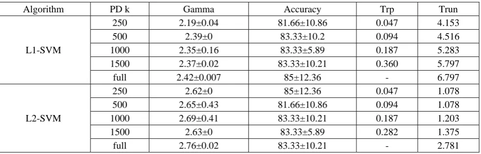
We describe experimental evaluations on Dbworkd and Arcene datasets. They both come from UCI database (http://archive.ics.uci.edu/ml/datasets.html) and satisfy n d_{. The results in Table 1-2 also} prove the proposed theorem because the maximum geometric margins and the testing accuracies are almost the same under different dimensions. In terms of running time, it is obvious that the RP-L1SVM takes more time than our RP-L2SVM on the two datasets.

Table 1. Results on dbworld dataset (644702)

Algorithm PD k Gamma Accuracy Trp Trun

L1-SVM

250 2.19±0.04 81.66±10.86 0.047 4.153

500 2.39±0 83.33±10.2 0.094 4.516

1000 2.35±0.16 83.33±5.89 0.187 5.283

1500 2.37±0.02 83.33±10.21 0.360 5.797

full 2.42±0.007 85±12.36 - 6.797

L2-SVM

250 2.62±0 85±12.36 0.047 1.078

500 2.65±0.43 81.66±10.86 0.094 1.078

1000 2.69±0.41 83.33±10.21 0.187 1.203

1500 2.63±0 83.33±5.89 0.282 1.375

Table 2. Results on arcene dataset (10010000)

Algorithm PD k Gamma Accuracy Trp Trun

L1-SVM

250 424.45±13.05 82.11±6 0.125 4.609

500 429.56±11.99 83.16±5.76 0.235 4.656

1000 451.58±8.17 85.26±7.81 0.453 4.063

1500 463.12±7.74 86.32±7.98 0.640 4.188

full 468.49±11.57 88.42±5.76 - 11.703

L2-SVM

250 411.48±22.62 85.26±5.76 0.109 2.516

500 444.46±9.16 87.37±2.88 0.234 2.266

1000 435.83±7.16 88.42±4.4 0.438 2.484

1500 466.02±8.1 91.57±7.98 0.640 2.689

full 471.71±12.11 89.47±6.45 - 7.734

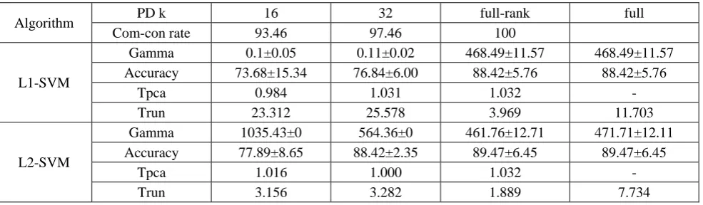
PCA vs. Random Projection

The PCA is one of the most widely used unsupervised dimensionality reduction techniques and its optimization problem is:

arg max /

w

w w X Xw w w

d k

T T T

tr







, where tr is the trace of a matrix, then the new data is X Xw , _Xn k _.

We do the experiment on Arcene dataset and use Matlab’s SVD solver in ‘econ’ mode to compute PCA. It is noticed that the number of principal components is less than or equal to the rank of the input matrix which is far less than the number of RPs.

What’s more, if the data matrix represented by a small number of principal components or random matrix combined with L2-SVM can have a better manifestation than that with L1-SVM. Here we use projected dimension k equal to 16, 32 and full-rank principal components and the cumulative contribution rate (‘Com-con rate’ in Table 3) is 93.46, 97.46 and 100.00 respectively, which is enough to represent the original data. The results of geometric margin in Table 3 indicate that PCA cannot preserve the geometry unchanged in contrast with RP (Table 2). In terms of accuracy and running time, PCA-L2SVM performs better than PCA-L1SVM in the same dimension. The performance of PCA-SVMs is dreadful than RP-SVMs excepting the condition of full-rank. The time of computing PCA is far more than RP, the same for PCA-SVMs compared with RP-SVMs.

Table 3. PCA experiments on arcene dataset.

Algorithm PD k 16 32 full-rank full

Com-con rate 93.46 97.46 100

L1-SVM

Gamma 0.1±0.05 0.11±0.02 468.49±11.57 468.49±11.57

Accuracy 73.68±15.34 76.84±6.00 88.42±5.76 88.42±5.76

Tpca 0.984 1.031 1.032 -

Trun 23.312 25.578 3.969 11.703

L2-SVM

Gamma 1035.43±0 564.36±0 461.76±12.71 471.71±12.11

Accuracy 77.89±8.65 88.42±2.35 89.47±6.45 89.47±6.45

Tpca 1.016 1.000 1.032 -

Trun 3.156 3.282 1.889 7.734

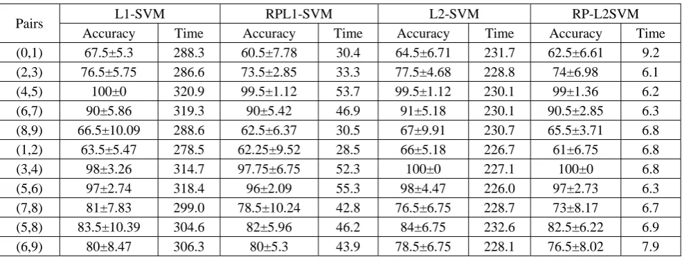
Application in Image Classification

Figure 1. The description of Corel images.

The results indicate that most of the RP-L2SVM accuracies are higher than RP-L1SVM. The accuracy of RP-L2SVM is comparable with L2-SVM. The total running time results show that our RP-L2SVM takes the least amount of time compared with L1-SVM, RP-L1SVM, L 2-SVM. The running time of our RP-L2SVM reduce at least five times compared with RP-L1SVM. All in all, our new RP-L2SVM has a better application in image classification.

Table 4. Accuracy and Time on Corel images.

Pairs L1-SVM RPL1-SVM L2-SVM RP-L2SVM

Accuracy Time Accuracy Time Accuracy Time Accuracy Time

(0,1) 67.5±5.3 288.3 60.5±7.78 30.4 64.5±6.71 231.7 62.5±6.61 9.2

(2,3) 76.5±5.75 286.6 73.5±2.85 33.3 77.5±4.68 228.8 74±6.98 6.1

(4,5) 100±0 320.9 99.5±1.12 53.7 99.5±1.12 230.1 99±1.36 6.2

(6,7) 90±5.86 319.3 90±5.42 46.9 91±5.18 230.1 90.5±2.85 6.3

(8,9) 66.5±10.09 288.6 62.5±6.37 30.5 67±9.91 230.7 65.5±3.71 6.8 (1,2) 63.5±5.47 278.5 62.25±9.52 28.5 66±5.18 226.7 61±6.75 6.8

(3,4) 98±3.26 314.7 97.75±6.75 52.3 100±0 227.1 100±0 6.8

(5,6) 97±2.74 318.4 96±2.09 55.3 98±4.47 226.0 97±2.73 6.3

(7,8) 81±7.83 299.0 78.5±10.24 42.8 76.5±6.75 228.7 73±8.17 6.7

(5,8) 83.5±10.39 304.6 82±5.96 46.2 84±6.75 232.6 82.5±6.22 6.9

(6,9) 80±8.47 306.3 80±5.3 43.9 78.5±6.75 228.1 76.5±8.02 7.9

Conclusion

This paper develops two significant theorems of L2-SVM under random projection. We prove that the geometric margin and the minimum enclosing ball in the projected space are preserved with high probability in the projected feature space in contrast with in the original space. The experimental results demonstrate the theory. Moreover, it is well applied in image classification problem. We hope our proposed method can inspire more work on extracting features effectively using RP under different SVMs.

References

[1] V.N. Vapnik, The nature of statistical learning theory, Springer, Berlin, 1995.

[2] J. Gu, L. Tao and H.K. Kwan, “Fast learning algorithms for new L2 SVM based on active set iteration method,” ISCAS, vol.5, 2004.

[4] C. Shi, et al., “Sparse feature selection based on L2, 1/2-matrix norm for web image annotation,” Neurocomputing, vol.151, 2015, pp.424-433.

[5] K. Pearson, “On Lines and Planes of Closest Fit to Systems of Points in Space,” Philosophical Magazine, vol.2, no.11, 1901, pp.559-572.

[6] W.B. Johnson and J. Lindenstrauss, “Extensions of Lipschitz maps into a Hilbert space,” In Contemp Math, vol.26, 1984, ppl.189-206.

[7] J. Maudes, et al., “Random projections for linear SVM ensembles,” Applied Intelligence, vol.34, no.3, 2011, pp. 347-359.

[8] S. Paul, et al., “Random Projections for Linear Support Vector Machines,” ACM Transactions on knowledge discovery from data, vol.8, no.224, 2014.

[9] P. Li and C. Zhang, “Compressed Sensing with Very Sparse Gaussian Random Projections,” AISTATS, 2015.

[10] D. Valsesia, et al., “Scale-robust compressive camera fingerprint matching with random projections,” ICASSP, 2015, pp. 1697-1701.