Applying a global optimisation algorithm to Fund of Hedge Funds portfolio optimisation

Munich Personal RePEc Archive

Applying a global optimisation algorithm

to Fund of Hedge Funds portfolio

optimisation

Thapar, Rishi and Minsky, Bernard and Obradovic, M and

Tang, Qi

19 August 2009

Online at

https://mpra.ub.uni-muenchen.de/17099/

Applying a global optimisation algorithm to

Fund of Hedge Funds portfolio optimisation

B. Minsky1, M. Obradovic2, Q. Tang2 and R. Thapar1

August 2009

Abstract:

Portfolio optimisation for a Fund of Hedge Funds (“FoHF”) has to address the

asymmetric, non-Gaussian nature of the underlying returns distributions. Furthermore, the objective functions and constraints are not necessarily convex or even smooth. Therefore traditional portfolio optimisation methods such as mean-variance optimisation are not appropriate for such problems and global search optimisation algorithms could serve better to address such problems. Also, in implementing such an approach the goal is to incorporate information as to the future expected outcomes to determine the optimised portfolio rather than optimise a portfolio on historic

performance.

In this paper, we consider the suitability of global search optimisation algorithms applied to FoHF portfolios, and using one of these algorithms to construct an optimal portfolio of investable hedge fund indices given forecast views of the future and our confidence in such views.

1

International Asset Management Ltd, 7 Clifford Street, London W1S 2FT, UK 2

Section 1: Introduction

The motivation for this paper was to develop a more robust approach to constructing portfolios of hedge fund investments that takes account of the issues that confront portfolio managers:

1. The non-Gaussian, asymmetric nature of hedge fund returns;

2. The tendency of optimisation algorithms to find corner solutions;

3. The speed in computation and efficiency in finding the solution; and

4. The desire to incorporate forecast views into the problem specification.

We describe here how each of these issues was addressed and illustrate with reference to the optimising of a portfolio of investable hedge fund indices. This paper synthesises a review of the applicability of global search optimisation algorithms for financial portfolio optimisation with the development of a Monte Carlo simulation approach to forecasting hedge fund returns and implementing the methodology into an integrated forecasting and optimisation application.

In Section 2, we summarise the review of global search optimisation algorithms and their applicability to the FoHF portfolio optimisation problem. In Section 3, we describe the Monte Carlo simulation technique adopted using resampled historical returns data of hedge fund managers and also how we incorporated forecast views and confidence levels, expressed as probability outcomes, into our returns distribution data. In Section 4, we report the results of applying the methodology to a FoHF portfolio optimisation problem and in Section 5, we draw our conclusions from the study.

Section 2: Review of global search optimisation algorithms

The FoHF portfolio optimisation problem is an example of the typical minimisation problem in finance

)

(

min

0 ) )( (

0 ) )( (

x

f

h x h

g x g

= <

= < M

Where f is non-convex and maybe non-smooth, called the objective function. The g, …, h are constraint functions, with g0, …, h0 as minimum thresholds. The variable x usually denotes the weights assigned to each asset and the constraints will usually include the buying and shorting limits on each asset.

optimisation the distribution of hedge fund returns are non-Gaussian and the typical objective functions and constraints are not limited to simple mean, variance and higher order moments of the distribution. We have previously [MOTT] discussed the use of performance and risk statistics such as maximum drawdown, downside deviation, co-drawdown, and omega as potential objective functions and constraint functions which are not obviously differentiable.

With the ready availability of powerful computing abilities and less demand on smoothness, it is possible to look for global optimisation algorithms which do not require regularity of the objective (constraint) functions to solve the financial minimisation problem.

In our review of the literature [MOTT], we found that there are three main ideas of global optimisation; Direct, Genetic Algorithm, and Simulated Annealing. In addition, there are a number of other methods which are derived from one or more of the ideas listed above.

A key characteristic of fund of fund portfolio optimisation, in common with other portfolio optimisation problems, is that the dimensionality of the problem space is large. Typically, a portfolio of hedge funds will have between 20 and 40 assets with some commingled funds having significantly more assets. This means that the search algorithm cannot conduct an exhaustive test of the whole space efficiently. For example, if we have a portfolio of 40 assets we have a 40-dimensional space, and an

initial grid of 100 points on each axis produces 1040 initial test points to evaluate the

region where the global minimum might be found. This would require considerable computing power and would not be readily feasible.

Each of the methods we considered in our review requires an initial search set. The choice of the initial search set is important as the quality of the set impacts the workload required to find the global minimum. The actual approach to moving from the initial set to finding better and better solutions differs across the methods and our search also revealed some approaches that combine the methods to produce a hybrid algorithm.

In [MOTT] we evaluated seven algorithms across the methods to identify which method and specific algorithm was best suited to our FoHF portfolio optimisation problem. The algorithms considered are described here:

1. PGSL: Probabilistic Global Search Lausanne

The search space is sampled using a probability distribution function for each axis of the multi-dimensional search space. At the outset of the search process, the probability distribution function is a uniform distribution with intervals of constant width. During the process, a probability distribution function is updated by increasing probability and decreasing the width of intervals of the regions with good functional values. A focusing algorithm is used to progressively narrow the search space by changing the minimum and maximum of each dimension of the search space.

2. MCS: Multi-level Co-ordinate Search

MCS belongs to the family of branch and bound methods and it seeks to solve bound constrained optimisation problems by combining global search (by partitioning the search space into smaller boxes) and local search (by partitioning sub-boxes based on desired functional values). In this way, the search is focused in favour of sub-boxes where low functional values are expected. The balance between global and local parts of the search is obtained using a multi-level approach. The sub-boxes are assigned a level, which is a measure of how many times a sub-box has processed. The global search part of the optimisation process starts with the sub-boxes that have low level values. At each level, the box with lowest functional value determines the local search process. The optimisation method is described in the paper by Huyer and Neumaier [HN].

Some of the finance papers that have examined MCS include [EG] and [KB]. In [EG] Value-at-Risk of a portfolio is calculated using marginal distributions of the risk factors and MCS is employed to search for the best-possible lower bound on the joint distribution of marginal distributions of the risk factors. [KB] uses MCS to optimise for Omega ratio, a non-smooth performance measure, of a portfolio.

3. MATLAB Direct:

The Direct Search algorithm, available in MATLAB’s Genetic Algorithm and Direct Search Toolbox, uses a pattern search methodology for solving bound linear or non-linear optimisation problems [M1]. The algorithms used are Generalised Pattern Search (GPS) and Mesh Adaptive Search (MADS) algorithm.

The pattern search algorithm generates a set of search directions or search points to approach an optimal point. Around each search point, an area, called a mesh, is formed by adding the current point to a scalar multiple of a set of vectors called a pattern. If a point in the mesh is found that improves the objective function at the current point, the new point becomes the current point for the next step and so on. The GPS method uses fixed direction vectors and MADS uses random vectors to define a mesh.

4. MATLAB Simulated Annealing:

model the physical process of heating a material and then slowly lowering the temperature to decrease defects, thus minimising the system energy [M1]. By analogy with this physical process, each step in the Simulated Annealing algorithm replaces the current point by another point that is chosen depending on the difference between the functional values at the two points and the temperature variable, which is systematically decreased during the process.

5. MATLAB Genetic Algorithm:

The MATLAB’s Genetic Algorithm is based on the principles of natural selection and uses the idea of mutation to produce new points in the search for an optimised solution [M1]. At each step, the Genetic Algorithm selects individuals at random from the current population to be parents and uses them to produce the children for the next generation. In this way, the population evolves toward an optimal solution.

6. TOMLAB LGO:

Tomlab’s Global Optimiser, TOMLAB/LGO, combines global and local search methodologies [T1]. The global search is implemented using the branch and bound method and adaptive random search. The local search is implemented using a generalised reduced gradient algorithm.

7. NAG Global Optimiser:

NAG’s Global Optimiser, E05JBF, is based on MCS, as described above. E05JBF is described in [N1] and [KB].

The above algorithms were evaluated on the three constrained optimisation problems described in paragraph 1.1 of Appendix I. The constraints consisted of both linear constraints on the allocation weights to the assets and constraints on the level of functions that characterise the portfolio’s performance or risk. The algorithms were measured regarding time to run, percentage of corners in the optimal solution, and the deviation from the average optimal solution. A simple scoring rule combining these three factors as a weighted sum was constructed and is also described in Appendix I.

Section 3: Implementing the Global Search Optimisation Algorithm

Traditional optimisation of portfolios has focused on determining the optimal portfolio given the history of asset returns and assuming that the distribution of returns is Gaussian and stationary over time. Our experience is that these assumptions do not hold and that any optimisation should use the best forecast we can make of the horizon for which the portfolio is being optimised. When investing in hedge funds, liquidity terms are quite onerous with lock ups and redemption terms from monthly to annual frequencies, and notice periods ranging from a few days to six months. This means that the investment horizon tends to be six to twelve months ahead to reflect the minimum time any investment will be in a portfolio.

The forecast performance of the assets within the portfolio is produced using Monte Carlo simulation and re-sampling. The objective is to produce a random sample of likely outcomes period by period for the forecast horizon based on the empirical distributions observed for the assets modified by our views as to the likely performance of the individual assets. This is clearly a non-trivial exercise, further complicated by our wish to maintain the relationship between the asset distributions and any embedded serial correlation within the individual asset distribution.

The approach implemented has three components:

1. Constructing a joint distribution of the asset returns from which to sample;

2. Simulating the returns of the assets over the forecast horizon; and

3. Calculating the relevant objective function and constraints for the optimisation.

Constructing the Joint Distribution of Asset Returns

We used bootstrapping in a Monte-Carlo simulation framework to produce the distribution of future portfolio returns. Bootstrapping is a means of using the available data by resampling with replacement. This generates a richer sample than would otherwise be available. To preserve the relationship between the assets we treat the set of returns for the assets in a time period as an observation of the joint distribution of the asset returns. An enhancement to this sampling scheme to capture any serial correlation is to block sample a group contiguously, say three periods together. Block sampling of three periods at a time offers around 10 million distinct samples of blocks of three time periods.

fund being approximately three years. Although the longer the range that can be used for the joint distribution the greater the number of points available for sampling, the lack of stationarity within the distribution leads us to select a compromise period, typically five years, as the desired range. Where a hedge fund does not have a complete five year history, we employed a backfill methodology to provide the missing data.

There are a number of approaches to backfilling asset return time series such as selecting a proxy asset to fill the series; using a strategy index with a random noise component; constructing a factor model of the asset returns from the available history and using the factor return history and model to backfill; or to randomly select an asset from a set of candidate assets that could have been chosen for the portfolio for the periods that the actual asset did not exist. We adopted this last method, selecting an asset from a set of available candidates within a peer group for the missing asset. Where the range for which returns are missing was long, we repeated the exercise of selecting an asset at random from the available candidates within the peer group, say, every six periods. Our reasoning for applying this approach is that we assume as portfolio managers, given the strategy allocation of the portfolio, that we would have chosen an asset from the candidate peer group available at that time to complete the portfolio. Using this process we constructed a complete set of returns for each of the assets going back, say, five years. The quality of the backfill depends on how narrowly defined the candidate peer group is defined. At International Asset Management Limited (IAM), we have defined our internal set of strategy peer groups that reflect best our own interpretation of the strategies in which we invest. This is because hedge fund classifications adopted by most of the index providers tend to be broad, and can include funds that would not feature in IAM’s classifications.

Simulating returns over the forecast horizon

We simulated the returns of the assets using a block bootstrap of the empirical joint distributions, which are modified by probabilistically shifting the expected return of the sample according to our assessment of the likely return outcomes for the assets. First we describe the process of incorporating forecast views by expectation shifting and then we describe the block bootstrapping method.

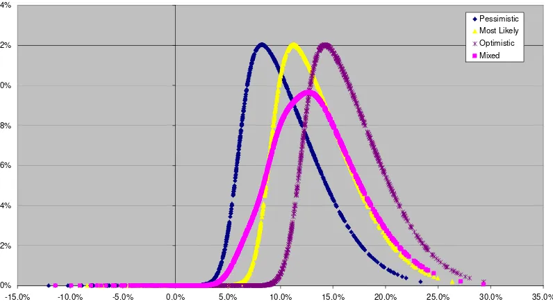
Figure 1 shows how applying a probabilistic shift to the mean of a distribution not only repositions the distribution but changes the higher order moments as the spread, skew and kurtosis all change.

Figure 1: Probabilistic Shifting of Expected Mean

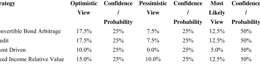
In Figure 2 the forecast views for a number of strategies are set out with associated confidence. The optimistic, pessimistic and most likely views are the best assessment of the potential expected return of the mean fund within the strategy. The confidence level represents the likelihood of that view prevailing. We note the sum of the three confidence levels is one. We use these likelihoods to determine for each asset, according to its strategy, which shift should be applied to the distribution for that simulation. This is implemented by simply sampling from the uniform distribution and dividing the distribution into three segments according to the confidence levels associated with the three views. Recognising that each asset does not track its strategy with certainty we calculate the beta for the asset with respect to the strategy and adjust the return by the randomly chosen shift (“k”) multiplied by the asset beta calculated. So the return in any period (“t”) for an asset (“a”) which follows strategy (“s”) for simulation trial (“n”) is:

m_ra,t,n = raw_r a,t,n + β x shifts,k

Impact of Mixing Views

0% 2% 4% 6% 8% 10% 12% 14%

Figure 2: Forecast views and confidence by hedge fund strategy

Strategy Optimistic View

Confidence / Probability

Pessimistic View

Confidence / Probability

Most Likely

View

Confidence / Probability

Convertible Bond Arbitrage 17.5% 25% 7.5% 25% 12.5% 50%

Credit 17.5% 25% 7.5% 25% 12.5% 50%

Event Driven 10.0% 25% 0.0% 25% 5.0% 50%

Fixed Income Relative Value 15.0% 25% 10.0% 25% 12.5% 50%

Calculating the objective function and constraint functions

In implementing the bootstrapped Monte Carlo simulation we simulate 500 trials or scenarios for the assets in the portfolio. This produces a distribution of returns of each asset and the distributions of any statistics we may wish to compute. Our objective and constraint functions are statistics based on the distribution of portfolio returns. With a set of asset allocation weights, the distribution of portfolio returns and statistics distributions may be calculated. It is worth discussing how we use this information within the optimisation algorithm. To do this we shall use as an example maximising expected return subject to a maximum level of maximum drawdown.

As we have chosen to optimise expected return, our objective function is simply the median of the distribution of portfolio returns. If we set our objective to ensure performance is at an acceptable level in most circumstances we might choose the bottom five percentile of return as the objective function so as to maximise the least likely (defined as fifth percentile) return. This reflects the flexibility we have with using a simulated distribution as the data input into the optimisation process.

In PGSL, as with almost all of the global search optimisation algorithms, both the linear and non-linear constraints are defined as penalty functions added to the objective function and hence are soft constraints rather than hard constraints that must be satisfied. The weight attached to each penalty function determines how acceptable a constraint violation is. In our example, we define the penalty function as the average of the maximum drawdown for the lowest five percentile of the maximum drawdown distribution less the constraint boundary assuming the conditional average exceeds the constraint level multiplied by an importance factor:

Max_dd_penalty =

- Max(Constraint_dd – average(Max_ddn | Lower 5%ile),0)

/ No. of Trials * Importance

Section 4: Results of Optimising a FoHF Portfolio

The approach to optimising a FoHF portfolio has been implemented in MATLAB and applied to a portfolio of eight RBC Hedge 250 hedge fund strategy indices. The monthly returns for indices from July 2005 are available from the RBC website. As the simulation requires five years of monthly returns the series were backfilled from the IAM’s pre-determined group of candidate assets within the relevant investment strategy peer group, using random selection as previously described. The results of the backfilling are shown in Appendix II.

The portfolio was optimised with an objective function to maximise median returns subject to constraints on the maximum and minimum allocations to each asset, a constraint on the maximum and minimum allocation to Long/Short Equity strategies and a maximum allowable maximum drawdown of 5% over the forecast horizon.

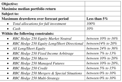
Thus the optimisation problem is as set out in Figure 3:

Figure 3: FoHF Portfolio Optimisation Problem

Objective: Maximise median portfolio return

Subject to:

Maximum drawdown over forecast period Less than 5%

• Total allocations for full investment 100%

• Cash 10%

Within the following constraints:

• RBC Hedge 250 Equity Market Neutral between 10% to 16% • RBC Hedge 250 Equity Long/Short Directional between14% to 20% • All Long/Short Equity between 24% to 36% • RBC Hedge 250 Fixed Income Arbitrage between 7% to 13% • RBC Hedge 250 Macro between 10% to 20% • RBC Hedge 250 Managed Futures between 10% to 20%, • RBC Hedge 250 Credit between 5% to 15% • RBC Hedge 250 Mergers & Special Situations between 0% to 10% • RBC Hedge 250 Multi-Strategy between 0% to 10%

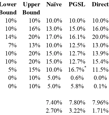
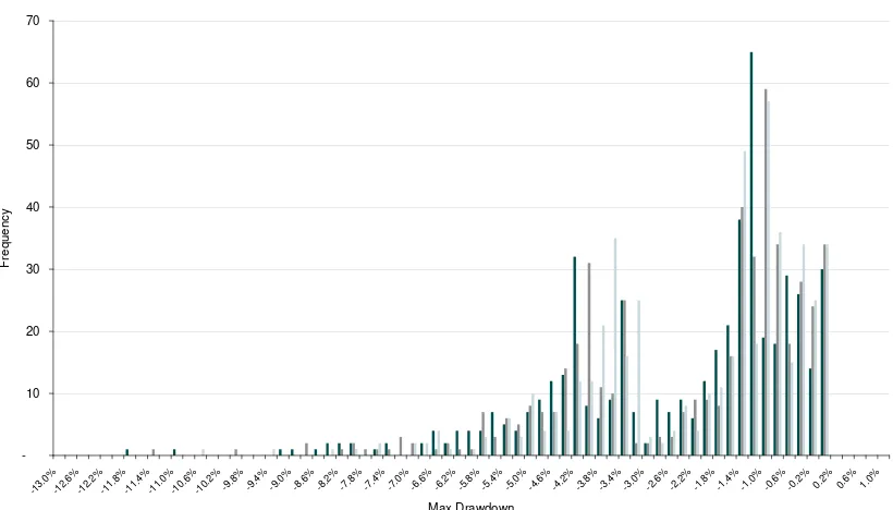
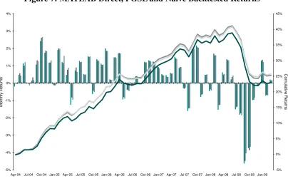
allocation). We noted that both optimisers improved median returns (7.8% and 8.0% vs. 7.40%) and that MATLAB Direct reduced the breach of the maximum drawdown constraint (1.71% vs. 2.70%) whereas the PGSL optimisation failed to improve on this condition (3.22% vs. 2.70%). The overall performance of the three portfolios is shown in Figures 4, 5, 6 and 7. Figure 5 shows the median and lower five percentile of the return distribution for both the two optimised portfolios. The returns and maximum drawdown distributions for the three portfolios are shown in Appendix III. In Figure 6, we compare the distributions of maximum drawdowns for the two optimised portfolios and the naïve portfolio. The graph shows that the MATLAB Direct portfolio had the better maximum drawdown distribution both in terms of worst case and general performance. Figure 7 shows the performance of the portfolios over the backtest period used in generating the data set. Again the MATLAB Direct optimised portfolio performs the best of the three portfolios. Finally we noted that PGSL optimisation terminated on maximum iterations and this might explain why it failed to meet all the allocation criteria.

Figure 4: Optimal Allocations and Results

Asset

Lower Bound

Upper Bound

Naïve PGSL Direct

Cash 10% 10% 10.0% 10.0% 10.0%

RBC Hedge 250 Equity Market Neutral 10% 16% 13.0% 15.0% 16.0%

RBC Hedge 250 Equity Long/Short 14% 20% 17.0% 16.1% 20.0%

RBC Hedge 250 Fixed Income Arbitrage 7% 13% 10.0% 12.5% 13.0%

RBC Hedge 250 Macro 10% 20% 15.0% 12.7% 13.9%

RBC Hedge 250 Managed Futures 10% 20% 15.0% 12.7% 15.4%

RBC Hedge 250 Credit 5% 15% 10.0% 16.7%* 11.5%

RBC Hedge 250 Mergers & Special Situations 0% 10% 5.0% 0.6% 0.0%

RBC Hedge 250 Multi-Strategy 0% 10% 5.0% 5.8% 0.1%

Median Return 7.40% 7.80% 7.96%

Excess Tail Maximum Drawdown 2.70% 3.22% 1.71%

Figure 5: MATLAB Direct, PGSL and Naïve Portfolios Returns

-4% -2% 0% 2% 4% 6% 8% 10%

Mar-09 Apr-09 May-09 Jun-09 Jul-09 Aug-09 Sep-09 Oct-09 Nov-09 Dec-09 Jan-10 Feb-10 Mar-10

A

n

nual R

etu

rn

(%)

Naïve Median Naïve 5%ile PGSL Median PGSL 5%ile Direct Median Direct 5%ile

Figure 6: MATLAB Direct, PGSL and Naïve Max Drawdown Distributions

-10 20 30 40 50 60 70

-13.0 %

-12.6 %

-12. 2%

-11. 8%

-11. 4%

-11.0 %

-10.6 %

-10.2 %

-9.8%-9.4%-9.0%-8.6%-8.2%-7.8%-7.4%-7.0%-6.6%-6.2 %

-5.8 %

-5.4 %

-5.0%-4.6%-4.2%-3.8%-3.4%-3.0%-2.6%-2.2%-1.8%-1.4%-1.0%-0.6 %

-0.2 %

0.2%0.6%1.0%

Max Drawdown

F

reque

ncy

Figure 7: MATLAB Direct, PGSL and Naïve Backtested Returns

-5% -4% -3% -2% -1% 0% 1% 2% 3% 4%

Apr-04 Jul-04 Oct-04 Jan-05 Apr-05 Jul-05 Oct-05 Jan-06 Apr-06 Jul-06 Oct-06 Jan-07 Apr-07 Jul-07 Oct-07 Jan-08 Apr-08 Jul-08 Oct-08 Jan-09

Mont

hly Ret

u

rns

-5% 0% 5% 10% 15% 20% 25% 30% 35% 40% 45%

C

o

m

u

la

ti

ve

R

e

tu

rns

Naïve Monthly PGSL Monthly Direct Monthly PGSL Cumulative Direct Cumulative Naïve Cumulative

Section 5: Conclusion

References:

[1] http://www.mat.univie.ac.at/~neum/ms/StArt.pdf

[2] http://www.andreassteiner.net/performanceanalysis/index.php

[BT] F Black and R Litterman, Asset Allocation: Combining Investor Views With

Market Equilibrium, Goldman, Sachs & Co., Fixed Income Research, September 1990

[CKM] S Ciliberti, I Kondor and M Mezard, On the Feasibility of Portfolio

Optimisation under Expected Shortfall, Quantitative Finance, 7(4), 2007, 389-396.

[CMLT] A Chabaane, J P Laurent, Y Malevergne and F Turpin, Alternative Risk

Measures for Alternative Investments, 21e Conference International en Finance, 2004.

[CUZ] A Chekhlov, S Uryasev and M Zabarankin, Drawdown Measure in Portfolio

Optimisation, International Journal of Theoretical and Applied Finance Vol. 8, No. 1 (2005) 13–58

[EG] Paul Embrechts, Giovanni Puccetti, Aggregating Risk Capital, with an

Application to Operational Risk, The GENEVA Risk and Insurance, Vol 31, Issue 2

[ET] I Ekeland and Roger Temam, Convex Analysis and Variational Problem,

Society for Industrial and Applied Mathematics, 1999.

[FREEDMAN] D A Freedman, Bootstrapping Regression Models, Ann Statist. 9,

1981, 1218-1228

[FS] G Fisher and A B Sim, Some Finite Sample Theory for Bootstrap Regression

Estimates, Journal of Statistical Planning and Inference 43, 1995, 289-300

[FV] C I Fabian and A Veszpremi, Algorithms for CVaR Optimisation in Dynamic

Stochastic Programming Models with Applications to Finance, Rutcor Research Report, RRR 24-2006, 09/2006

[GKH] M Gilli, E Kellezi and H Hysi, A Data-Driven Optimisation Heuristic for

Downside Risk Minimisation, Journal of Risk, 8(3), 2006, 1-19.

[HN] W Huyer and A Neumaier, Global Optimisation by Multilevel Coordinate

Search, J. Global Optimisation 14, 1999, 331-355.

[HUYER] W Huyer, A Comparison of Some Algorithms for Bound Constrained

[HWRSVJBT] J. He, L. T. Watson, N. Ramakrishnan, C. A. Shaffer, A. Verstack, J

Jiang, K. Bae and W. H. Tranter, Dynamic Data Structures for a Direct Search

Algorithm, Computational Optimisation and Applications, 23, 2002, 5–25

[KB] S.J. Kane and M.C. Bartholomew-Biggs, Optimising Omega, Journal of Global

Optimisation, Vol 45, Number 1.

[KK] A I Kibzun and E A Kuznetsov, Comparison of VaR and CVaR Criteria,

Automation and Remote Control, 64(7), 2003, 1154-1164

[KK1] P D Kaplan and J A Knowles, Kappa: A Generalised Downside Risk-Adjusted

Performance Measure, Journal of Performance Measurement, Spring 2004.

[KPU] P Krokhmal and S Uryasev, Portfolio Optimisation with Conditional

Value-at-Risk Objective and Constraints, The Journal of Risk, 4(2), Winter 2001/02.

[KS] C Keating and W F Shadwick, A Universal Performance Measure,

http://www.spgshop.com/index.asp?PageAction=VIEWPROD&ProdID=413.

[KSG] H Kazemi, T Schneeweis and R Gupta, Omega as a performance measure,

http://www.edhec-risk.com/site_edhecrisk/public/research_news/choice/RISKReview1 063631261806712604, 2003.

[M1] Genetic Algorithm and Direct Search Toolbox™ 2 User’s Guide, Mathworks, http://www.mathworks.com/access/helpdesk/help/pdf_doc/gads/gads_tb.pdf

[MOTT] B Minsky, M Obradovic, Q Tang and R Thapar, Global Optimisation

algorithms for financial portfolio optimisation, Working Paper University of Sussex, 2008

[MP] D Martinger and P Parpas, Global Optimisation of Higher Order Moments in

Portfolio Selection, J Glob Optim, 2007.

[MSRY] L Mitra, X Sun, D Roman, G Mitra & K Yu, Mixture distribution scenarios

for investment decisions with downside risk, Working Paper, SSRN, June 2009

[N1] NAG Library Routine Document E05JBF, NAG,

http://www.nag.co.uk/numeric/FL/nagdoc_fl22/pdf/E05/e05jbf.pdf

[PFLUG] G Ch Pflug, Some Remarks on the Value-at-Risk and the Conditional

[RABER] U Raber, A Simplicial Branch-and-Bound Method for Solving Nonconvex All-Quadratic Programs, Journal of Global Optimisation, 13, 1998, 417-432.

[RS] B Raphael and I F C Smith, A Direct Stochastic Algorithm for Global Search,

Applied Mathematics and Computation, 146, 2003, 729-758

[RU] R T Rockafellar and S Uryasev, Optimisation of Conditional Value-at-Risk,

Journal of Risk, 2(3), 2000, 21-41.

[RUZ] R T Rockafellar, S Uryasev and M Zabarankin, Deviation Measure in Risk

Analysis and Optimisation (December 22, 2002). University of Florida, Department of Industrial & Systems Engineering Working Paper No. 2002-7. Available at SSRN: http://ssrn.com/abstract=365640.

[RUZ1] R T Rockafellar, S Uryasev and M Zabarankin, Optimality Conditions in

Portfolio Analysis with General Deviation Measures (May 10, 2005). University of Florida Industrial and Systems Engineering Working Paper No. 2004-7. Available at SSRN: http://ssrn.com/abstract=615581

[T1] User’s guide for TOMLAB/ LGO1TOMLAB http://tomopt.com/docs/TOMLAB_LGO.pdf

[WM] P Winker and D Maringer, The Threshold Accepting Optimisation Algorithms

in Economics and Statistics, in: Kontoghiorges, E.J., Gatu, Chr. (eds.), Optimisation, Econometric and Financial Analysis, Springer, 2007.

[YYSL] X Yang, Z Yang, Z Shen and G Lu, Gray-Encoded Hybrid Accelerating

Appendix I: Tests of Algorithms with Objective Function and Constraints

1.1 Specifications of Problems with Objective and Constraint Functions

1) Constrained Optimisation-1: Maximising compounded annualised return subject to

x1+ …+ xn =1

Annualised Volatility ≤5%

Max Drawdown ≤7%

Co-drawdown (to MSCI index) ≤60%

Allocation between 0 and 15% of portfolio

2) Constrained Optimisation-2: Minimise annualised volatility subject to

x1+ …+ xn =1

Compounded Annualised Returns ≥10% and

Max Drawdown ≤7%

Co-drawdown (to MSCI index) ≤60%

Allocation between 0 and 15% of portfolio

3) Constrained Optimisation-3: Maximise Omega ratio subject to

x1+ …+ xn =1

Compounded Annualised Returns ≥10%

Max Drawdown ≤7%

Annualised Volatility ≤5%

Co-drawdown (to MSCI World index) ≤60%

Allocation between 0 and 15% of portfolio

1.2 Aggregate Scoring Function:

For a fixed number of assets, scoring measure, r , is calculated as:

r= *0.7 *0.2

eSpent AverageTim

Spent ActualTime eSpent

AverageTim AverageMin

ActualMin

AverageMin − ₊ −

-0.1*

asset of Nr total

15% or 0 either is allocation output

the times of Nr

The higher the value, the better the algorithm is.

The first term in the formula above is about the minimum we achieved:

AverageMin = average of all minimums found by all algorithms

The second term considers the time taken to find a solution:

AverageTimeSpent = average time spent by all algorithms

ActualTimeSpent = time spent by the algorithm investigated

The last term takes care of the undesirable corner solutions (i.e. optimised allocations at either of min or max asset allocation bounds).

Each algorithm was numerically tested for 10 assets, 20 assets, 30 assets and 40 asset

cases (r₁₀, r₂₀, r₃₀ and r₄₀) and a weighted score is obtained as:

r = 0.1 * r₁₀ + 0.2 * r₂₀ + 0.3 * r₃₀ + 0.4 * r₄₀.

This final r, depends on algorithm and constrained optimisation setup, is used to quantitatively evaluate the algorithms.

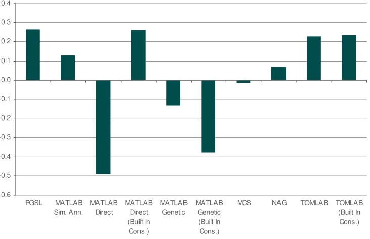
The weighted scores of the seven algorithms for the three constrained optimisation setups are given below:

Figure 1: Weighted Score for Constrained Optimisation-1

-1.0 -0.8 -0.6 -0.4 -0.2 0.0 0.2 0.4

PGSL MATLAB

Sim. Ann.

MATLAB Direct

MATLAB Direct (Built In

Cons.)

MATLAB Genetic

MATLAB Genetic (Built In Cons.)

MCS NAG TOMLAB TOMLAB

Figure 2: Weighted Score for Constrained Optimisation-2

-1.0 -0.8 -0.6 -0.4 -0.2 0.0 0.2 0.4

PGSL MATLAB

Sim. Ann.

MATLAB Direct

MATLAB Direct (Built In Cons.)

MATLAB Genetic

MATLAB Genetic (Built In Cons.)

MCS NAG TOMLAB TOMLAB

(Built In Cons.)

Figure 3: Weighted Score for Constrained Optimisation-3

-0.6 -0.5 -0.4 -0.3 -0.2 -0.1 0.0 0.1 0.2 0.3 0.4

PGSL MATLAB

Sim. Ann.

MATLAB Direct

MATLAB Direct (Built In

Cons.)

MATLAB Genetic

MATLAB Genetic (Built In Cons.)

MCS NAG TOMLAB TOMLAB

Appendix II: RBC Hedge 250 Strategy Indices Backfilled to June 2005 Equity Market Neutral Fixed Income Arbitrage Equity Long/Short Macro Managed Futures

Credit Mergers &

Special Situations

Multi-Strategy

Apr-04 0.01% 2.01% 0.32% -4.43% 0.18% 1.80% -0.20% 0.18% May-04 -0.90% -1.15% -1.13% -0.59% 7.10% -0.64% -0.06% -0.36% Jun-04 0.70% -0.10% 3.31% 4.40% -1.42% 0.43% -0.08% 0.00% Jul-04 -1.00% -1.91% -1.73% 1.71% 1.33% 1.45% -0.29% 0.37% Aug-04 0.26% 0.06% 0.62% -5.36% 4.10% 0.85% 0.51% 1.30% Sep-04 0.30% 1.07% 2.40% -4.15% 6.74% 1.04% -0.27% 0.48% Oct-04 8.12% 0.45% 1.82% 0.40% 5.65% -0.04% 1.30% 0.67% Nov-04 0.69% 6.03% 2.24% -2.38% 5.22% -0.04% 3.92% 0.79% Dec-04 2.72% 0.51% 3.16% -0.59% 0.75% 1.11% 1.40% 0.26% Jan-05 -0.22% 0.00% -0.88% 1.12% -1.01% 0.50% -0.46% 0.07% Feb-05 4.43% 2.07% 2.91% 0.99% 3.47% -2.41% 1.37% 2.38% Mar-05 1.47% -0.72% 4.21% -0.03% 3.29% 0.62% 1.13% -5.05% Apr-05 1.60% -0.42% 1.60% -0.37% 2.82% -0.34% -5.38% -0.93% May-05 -0.70% -0.04% -1.41% -8.10% 2.82% 0.99% -4.27% -0.58% Jun-05 1.04% 1.52% 0.46% -6.20% 6.95% -0.34% 3.43% 1.70% Jul-05 0.30% 1.03% 2.53% 1.34% 0.73% 1.89% 2.09% 1.61% Aug-05 0.53% 0.31% 1.43% 0.66% -0.82% 0.88% 0.96% 0.86% Sep-05 1.40% 0.23% 1.97% 3.13% 1.82% 1.26% 1.02% 1.43% Oct-05 -0.77% 0.74% -2.47% -0.78% 0.78% -0.25% -2.96% -0.64% Nov-05 -0.67% -0.10% 2.24% 1.76% 4.09% 0.48% 1.80% 0.94% Dec-05 1.41% 0.50% 2.59% 1.23% -0.47% 1.15% 1.72% 2.03% Jan-06 -0.17% 0.64% 3.74% 2.86% 2.02% 2.62% 3.15% 2.86% Feb-06 -0.01% 0.43% 0.45% 0.12% -0.84% 1.04% 0.75% 0.75% Mar-06 1.62% 0.49% 2.47% 0.14% 2.73% 1.34% 1.69% 2.27% Apr-06 1.13% 1.19% 1.78% 1.91% 3.53% 1.47% 1.48% 1.72% May-06 -0.57% 0.64% -2.21% -2.70% -0.60% -0.11% -1.26% -0.50% Jun-06 -0.85% 0.32% -0.85% -0.30% -0.54% -1.05% 0.34% 0.38% Jul-06 0.80% 0.66% 0.12% -0.87% -2.00% 0.37% -0.18% 0.15% Aug-06 -0.03% -0.11% 1.41% -1.17% 0.78% 0.89% 0.78% 1.22% Sep-06 -0.04% 0.31% 0.13% -0.97% -0.44% 0.41% 0.23% 0.50% Oct-06 0.42% 0.68% 2.33% 0.59% 1.73% 1.61% 1.71% 1.39% Nov-06 0.67% -0.18% 2.16% 0.71% 2.65% 1.63% 1.86% 1.64% Dec-06 0.53% 0.84% 1.44% 1.06% 2.16% 1.52% 1.89% 1.66% Jan-07 1.00% -0.06% 1.05% 0.23% 1.63% 1.29% 2.52% 1.85% Feb-07 1.63% 0.80% 0.67% 0.34% -1.69% 1.00% 1.86% 1.62% Mar-07 0.62% 0.29% 1.56% 0.08% -1.15% 0.42% 2.11% 1.02% Apr-07 1.05% 0.91% 1.19% 0.45% -1.04% 0.78% 1.50% 1.21% May-07 1.04% 0.05% 1.79% 1.79% 2.69% 1.35% 2.73% 1.78% Jun-07 0.84% -0.32% 0.86% 1.48% 2.52% 0.30% -0.93% 0.54% Jul-07 0.23% 0.71% 0.22% -0.26% -2.39% -0.71% 0.19% -0.30% Aug-07 -0.78% 0.78% -1.07% -4.43% -3.07% -1.31% -2.24% -1.44% Sep-07 0.43% 1.70% 2.25% 2.69% 4.38% 1.35% 1.04% 1.28% Oct-07 0.67% 0.43% 3.02% 2.78% 4.15% 1.74% 3.10% 2.31% Nov-07 -0.13% -0.88% -1.23% -1.25% 0.28% -1.35% -3.07% -1.71% Dec-07 -0.14% 0.65% 0.74% 1.17% 0.46% 0.22% -0.37% 0.26% Jan-08 -3.06% 0.15% -3.43% 2.73% 3.09% -1.41% -3.96% -1.52% Feb-08 0.99% -0.65% 2.29% 1.98% 4.81% 0.31% 2.92% 0.57% Mar-08 -0.88% -1.69% -1.73% -3.48% 0.99% -2.09% -5.58% -2.33% Apr-08 0.79% 0.02% 1.71% 1.26% -1.23% 0.50% 1.97% 0.98% May-08 1.67% 0.18% 2.40% 1.15% 1.58% 1.06% 2.10% 1.87% Jun-08 1.95% -0.56% -0.62% 0.65% 1.80% -0.58% -2.34% -1.63% Jul-08 -2.25% 1.68% -2.75% -1.12% -1.87% -2.03% -3.14% -2.51% Aug-08 -1.40% 0.69% -1.29% -4.77% -1.84% -4.60% -0.60% -0.42% Sep-08 -2.29% -7.64% -6.37% -4.65% 1.05% -8.12% -8.37% -14.73% Oct-08 0.81% -14.40% -4.86% -0.67% 3.29% -12.12% -5.93% -10.01% Nov-08 -0.43% -2.87% -1.25% -0.26% 3.12% -5.26% -2.30% -4.63% Dec-08 0.24% -1.02% -0.13% 1.31% 1.73% -4.02% -0.32% -0.87% Jan-09 2.69% 1.90% 0.71% 1.16% 1.97% -0.59% 1.69% 2.76% Feb-09 -0.52% -0.29% -1.09% -1.42% -0.13% -1.37% -0.83% -0.57% Mar-09 0.27% 1.26% 0.71% 1.48% -2.24% -0.15% 0.57% 0.44%

Appendix III: Comparison of Naïve and Optimised Portfolios

Naïve Portfolio

Naïve Portfolio: Annualised Returns

0 5 10 15 20 25 30 35 40 45 50

-11%-10% -9% -8% -7% -6% -5% -4% -3% -2% -1% 0% 1% 2% 3% 4% 5% 6% 7% 8% 9% 10%11% 12% 13% 14% 15% 16% 17% 18%19%20%

F

re

que

nc

y

Naïve Portfolio: Maximum Drawdown

Optimised Portfolio: PGSL

Optimised Portfolio: Annual Returns

0 5 10 15 20 25 30 35 40 45 50

-10% -8% -6% -4% -2% 0% 2% 4% 6% 8% 10% 12% 14% 16% 18% 20%

F

requenc

y

Optimised Portfolio: Maximum Drawdown

0 10 20 30 40 50 60 70

-12.0% -11.2% -10.4% -9

Optimised Portfolio: MATLAB Direct

Optimised Portfolio: Annualised Returns

0 10 20 30 40 50 60

-10% -8% -6% -4% -2% 0% 2% 4% 6% 8% 10% 12% 14% 16% 18% 20%

F

requenc

y

Optimised Portfolio: Maximum Drawdown

0 10 20 30 40 50 60

-11.0%-10.2% -9 .4%

-8.6 %

-7.8 %

-7.0%-6.2%-5.4 %

-4.6 %

-3.8%-3.0%-2.2 %

-1.4 %

-0.6 %

0.2% 1.0%

F

reque

nc