A Toolbox for Exoplanet Exploration

(1)

Thesis by

Rebecca Jensen-Clem

In Partial Fulfillment of the Requirements for the

Degree of

Doctor of Philosophy

CALIFORNIA INSTITUTE OF TECHNOLOGY

Pasadena, California

2017

(2)

Rebecca Jensen-Clem ORCID: 0000-0003-0054-2953

(3)

ACKNOWLEDGEMENTS

I can only begin this thesis by thanking my parents and sister for their unending love

and support. From the first living room conversation about black holes, to book

signings, to keeping me sane as a harried student, I couldn’t ask for better guides

through this strange cosmos.

This thesis is also made possible by my many wonderful mentors in high school

and college. I would like to thank Steve Murphy, John Heil, Peter Saxby, David

Trowbridge, and Don McCarthy for encouraging my early interest in astronomy and

helping me build a foundation of physics. At MIT, I was fortunate to learn from Jim

Elliot, Matt Smith, and Sara Seager; I will always be grateful for their mentorship

and generosity.

At Caltech, I’ve had the amazing good fortune of being advised by Shri Kulkarni.

I can’t imagine grad school without his wisdom and perspective, and I’m a better

scientist for having him as an example. I am also grateful to have had the opportunity

to work with Dimitri Mawet. His expertise, open door, and encouragement have

been a continuous source of positivity. Thank you to Lynne Hillenbrand, Sterl

Phinney, and Evan Kirby for many useful conversations and support throughout grad

school. Thank you also to Kent Wallace for continuous mentorship and friendship

throughout my time at Caltech.

I would also like to thank the many collaborators who have enriched the science in

this thesis, among them Mike Bottom, Phil Muirhead, Ben Mazin, Seth Meeker, Rich

Dekany, Jennifer Milburn, Carlos Gomez Gonzalez, Olivier Absil, James Graham,

Max Miller-Blanchaer, Dmitry Duev, Reed Riddle, Christoph Baranec, and the staff

at Palomar, Kitt Peak, and Keck Observatories.

I would like to thank my wonderful friends and fellow astro grads for always being

there with movie nights, gym classes, and Red Door trips. In particular, I’d like to

thank Marta Bryan: the best friend, officemate, and possible twin I could ever ask

for.

(4)

ABSTRACT

In this thesis, I develop a new suite of tools to address two questions in exoplanet

science: how common are Earth-mass planets in the habitable zones of Solar-type

stars, and can we detect signs of life on other worlds?

Answering the first question requires a method for detecting Earth-Sun analogs.

Currently, the radial velocity (RV) method of exoplanet detection is one of the

most successful tools for probing inner planetary systems. However, degeneracy

between a spectrometer’s wavelength calibration and the astrophysical RV shift has

limited the sensitivity of today’s instruments. In my thesis, I address a method

for breaking this degeneracy: by combining a traditional spectrometer design with

a dynamic interferometer, a fringe pattern is generated at the image plane that is

highly sensitive to changes in the radial velocity of the target star. I augmented

previous theoretical studies of the method, creating an end-to-end simulation to 1)

introduce and recover wavelength calibration errors, and 2) investigate the effects

of interferometer position errors on the RV precision. My simulation showed that

using this kind of interferometric system, a 5-m class telescope could detect an

Earth-Sun analog.

Addressing the occurrence rate of Earth twins also requires an understanding of

planet formation in multiple star systems, which encompass half of all Solar-type

stars. Gravitational interactions between binary components separated by 10 −

100 AU are predicted to truncate the outer edges of their respective disks, possibly

reducing the disks’ lifetimes. Consequently, the pool of material and the amount of

time available for planet formation may be smaller than in single star systems. The

stars’ rotational periods provide a fossil record of these events: star-disk magnetic

interactions initially prevent a contracting pre-main sequence star from spinning

up, and hence a star with a shorter-lived disk is expected to be spinning more

quickly when it reaches the zero age main sequence. In order to conduct a

large-scale multiplicity survey to investigate the relationship between stellar rotation and

binary system properties (e.g. their separations and mass ratios), I contributed to

the commissioning of Robo-AO, a robotic laser guide star adaptive optics system,

at the Kitt Peak 2.1-m. After the instrument’s installation, I wrote a data pipeline

to optimize the system’s sensitivity to close stellar companions via reference star

differential imaging. I then characterized Robo-AO’s performance during its first

(5)

stars in the Pleiades with rotational periods measured using the photometric data of

the re-purposed Kepler telescope, K2.

Detecting signs of life on other worlds will require detailed characterization of

rocky exoplanet atmospheres. Polarimetry has long been proposed as a means of

probing these atmospheres, but current instruments lack the sensitivity to detect

the starlight reflected and polarized by such small, close-in planets. However, the

latest generation of high contrast imaging instruments (e.g. GPI and SPHERE) may

be able to detect the polarization of thermal emission by young, gas giants due to

scattering by aerosols in their atmospheres. Observational constraints on the details

of clouds physics imposed by polarized emission will improve our understanding

of the planets’ compositions, and hence their formation histories. For the case of

the brown dwarf HD19467 B orbiting a nearby Sun-like star, I demonstrated that

the Gemini Planet Imager can detect linear polarizations on the order predicted for

these cloudy exoplanets. My current pilot programs can produce the first detections

of polarized exoplanet emission, while also building expertise for reflected starlight

(6)

PUBLISHED CONTENT AND CONTRIBUTIONS

Jensen-Clem, R., D. A. Duev, et al. (2017). “The Performance of the Robo-AO Laser Guide Star Adaptive Optics System at the Kitt Peak 2.1-m Telescope”. In:ArXiv e-prints. arXiv:1703.08867 [astro-ph.IM].

R. J.-C. contributed to the installation of the instrument, developed the faint star pipeline, developed the high contrast pipeline, contributed to the analysis of the weather and telescope jitter data, and contributed to the preparation of the manuscript.

Jensen-Clem, R., D. Mawet, et al. (2017, Submitted). “A New Standard for Assess-ing the Performance of High Contrast ImagAssess-ing Systems”. In: The Astronomical Journal_.

R. J.-C. participated in the conception of the project, performed the analysis, and prepared the manuscript.

Jensen-Clem, R., M. Millar-Blanchaer, et al. (2016). “Point Source Polarimetry with the Gemini Planet Imager: Sensitivity Characterization with T5.5 Dwarf Companion HD 19467 B”. In:The Astrophysical Journal 820, 111, p. 111. doi:

10.3847/0004-637X/820/2/111_{. arXiv:}1601.01353 [astro-ph.EP]_.

R. J.-C. participated in the conception of the project, performed the post-GPI-pipeline data analysis, and prepared the manuscript.

Jensen-Clem, R., P. S. Muirhead, et al. (2015). “Attaining Doppler Precision of 10 cm s−1with a Lock-in Amplified Spectrometer”. In:Publications of the Astronomical Society of the Pacific_{127, p. 1105. doi:}10.1086/683796_{. arXiv:}1510.05602

[astro-ph.IM]_.

(7)

LIST OF ILLUSTRATIONS

Number Page

1.1 The masses and separations of all exoplanets detected as of April

24th, 2017. The red points show planets detected using transits, the

blue points radial velocities, the green points microlensing, and the

magenta points direct imaging. This figure was generated using the

Exoplanet Data Explorer at exoplanets.org (Han et al 2014). . . 2

1.2 A star (large filled circle) and planet (small black circle) are shown

orbiting their mutual center of mass (black cross), with the star’s

spectrum represented schematically at the top of each panel. The

observer is located at the bottom of the figure. When the star’s

velocity is entirely horizontal on the page, the observer sees no shift in

the spectral features (first and third panels). When the star is moving

away from the observer, the star’s spectral features are redshifted

(second panel). When the star is moving towards the observer, its

spectral features are blueshifted (fourth panel). Hence, the periodic

red and blue shift of the star’s spectral features reveal the gravitational

influence of the planet. . . 3

1.3 An illustration of a three dimensional Keplerian orbit. The labeled

parameters are described in the main text. This figure is adopted

from M. Perryman (2011). . . 3

1.4 A schematic illustration of the transit method of exoplanet detection

and atmospheric characterization. Panel (a) shows a cartoon of a

transit event as a planet passes in front of its host star. This event

corresponds to the first flux diminution in the plot of stellar flux

versus planet phase in panel (b). The second, smaller diminution

corresponds to the occultation event. This figure is adapted from S.

Seager and Deming (2010). . . 6

1.5 The flux as a function of wavelength for a solar system analog at 10

pc. This figure is adapted from S. Seager and Deming (2010). . . 8

1.6 The luminosity of stars, brown dwarfs, and planets are plotted as a

function of age. Several directly imaged exoplanets are overplotted.

(10)

1.7 The absolute H−band magnitude is plotted as function of J − K

color for various stars and brown dwarfs. Several directly imaged

exoplanets are overplotted, with their color indicating their spectral

type. This figure is adapted from B. P. Bowler (2016). . . 11

1.8 A circular aperture whose center is located at a distance R from a

point of observationP(not to scale). This figure is inspired by Figure

4.2 in Hardy 1998. . . 12

1.9 A schematic of an adaptive optics system. . . 13

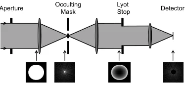
1.10 A schematic of a Lyot coronagraph optical setup. The lower part

of the figure indicates the intensity patterns at the entrance pupil,

first focal plane, second “Lyot" pupil plane, and second focal plane

(Guyon, C. Roddier, et al. 1999, ©The Astronomical Society of the

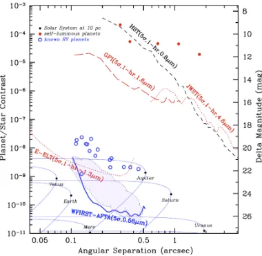
1.11 The planet-to-star contrast ratios achieved by current and future planet

imaging instruments (black, red, and bold blue lines). Several young,

massive planets that have already been detected in the near infrared

are shown by the red dots. The open blue circles represent the

visible-wavelength contrast ratios of planets that have been detected by the

radial velocity method, but have not yet been directly imaged. The

solar system planets at visible wavelengths are shown as black dots,

with the thin blue curves representing different phase angles. This

figure was adapted from Spergel et al. (2015). . . 19

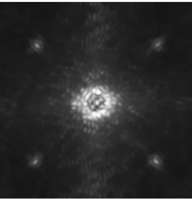
1.12 An example of a post-AO, post-coronagraphic stellar point spread

function (P1640/Nilsson, private communication). Many bright

“speckles” are visible around the attenuated star in the center of

the image. The speckles are slightly elongated due to the wide

band-pass of the image (λ0 = 1.3µm, ∆λ = 25 nm). The four bright

speckles are intentionally created in order to provide astrometric and

photometric calibration sources. . . 20

2.1 A horizontal cut through Figure 2.2 reveals the simulated stellar

spectrum. Note that for ease of viewing, Figure 2.2 shows the mean

(11)

2.2 A simulated mean subtracted spectrum vs. wavelength and ∆τ for

SNR = 500. The x-axis corresponds to wavelength, or pixels on

the spectrometer detector. The y-axis corresponds to changes in the

optical path difference of the interferometer, and therefore represents

time as the interferometer optical path difference is modulated

tem-porally. The regions of high fringe contrast correspond to absorption

lines in the stellar spectrum. An error in the wavelength calibration

is fundamentally different from a change in the radial velocity of the

target star, as long as the wavelength calibration error does not occur

during an interferometer scan. . . 33

2.3 Simulated likelihood contours describing the radial velocity and

wavelength calibration error reconstructions for injected values of

1000 m s−1and 500 m s−1respectively, for SNR=100 and a spectral bandwidth of∆λ=88Å. In contrast to traditional RV reconstruction

methods, the contours show an elliptical shape, demonstrating that

the RV and wavelength calibration error measurements are not highly

correlated. . . 35

2.4 Radial velocity precision is plotted against the signal-to-noise ratio

for Poisson noise limited measurements, (no instrumental or

astro-physical noise sources). Under these conditions, an SNR of about 94

per phase step, for 200 phase steps, is required to reach a precision

of 10 cm s−1. The RV precisions shown in this plot were calculated using a spectral bandwidth of∆λ=88Å, and were divided by

√

10 to

reflect the RV precisions associated with the fullV-band bandwidth

of 880Å. . . 36

2.5 The radial velocity precision is shown to be approximately constant

over 10 km s−1 (∼ 0.2Å) wavelength calibration errors for SNR = 10, 100, and 1000. In contrast, the radial velocity precision is

pro-portional to the wavelength calibration error in conventional

spec-troscopy. The RV precisions shown in this plot were calculated using

a spectral bandwidth of∆λ= 88Å, and were divided by

√

10 to reflect

(12)

2.6 The RV precision is plotted against the standard deviation of the phase

step error. The horizontal dotted lines represent the Poisson limited

RV precision for each SNR. In the phase step error limited regions,

the RV precisions approach the limitingSN R= ∞condition, shown

by the black line. For SNR = 100,∆τmust be measured to less than

1 nm to reach the Poisson limited regime. Because the phase step

errors are assumed to be uncorrelated, the total number of phase steps

affects the final RV precision. In this simulation, we chose 200 steps

(Table 2.1). The RV precisions shown in this plot were calculated

using a spectral bandwidth of∆λ=88Å, and were divided by

√

10 to

reflect the RV precisions associated with the fullV-band bandwidth

of 880Å. . . 38

3.1 The reduced Stokes images with the ring of comparison apertures

superimposed (the white arrow indicates the companion in Stokes I).

The companion’s SNR (Equation 3.1) is 7.4 in Stokes I, but SNR< 1.0

in Stokes Q and U. Hence, no polarized radiation is detected from the

companion. . . 49

3.2 Histograms of the summed counts in the Stokes comparison

aper-tures. The aperture size is equal to the full width at half maximum

of the companion (3.44 pixels, or 0.049"). The Stokes I histogram

(a) has an excess of higher values due to speckle noise. Because HD

19467 A is an unpolarized star, there is little flux at the companion’s

separation in the Q and U frames. The large spread in Q and U values

is due in part to the small number of apertures used (66). . . 51

3.3 The probability density function of p =

√

Q2₊U2

I , via Equation 3.6. The four fits are to skewed Gaussian, Rayleigh, Rice, and Hoyt

distri-butions. All but the skewed Gaussian are special cases of Equation

3.4 for different values of the means and standard deviations ofQand

U. The best fit is the Hoyt distribution. . . 55

(13)

4.2 (a) The normally distributed PDF of a noise source with a mean of

zero and standard deviation of one. Here, the detection criterion is

arbitrarily set to 3σ (dashed line), which corresponds to x = 3 for

this distribution. Because the noise PDF falls above the detection

threshold a fraction 0.001 of the time, the false positive fraction in

this example is 0.001. (b) The Gaussian PDF of a signal source with

a mean of x =3 and a standard deviation of one. Because half of the

signal distribution’s area falls above the detection criterion, the true

positive fraction is 0.5. . . 63

4.3 Black line: an ROC curve corresponding to a range of criteria applied

to the noise and signal distributions in Figure 4.2. The (TPF, FPF)

locations corresponding to criteria of 1σ−3σare labeled to

demon-strate the trade-offs between these key parameters. We note that FPF

values larger than 0.5 require a criterion that is less than the mean

of the noise distribution. Because the noise is normally distributed

in this example, such criteria are negative. Grey line: the equivalent

ROC curve for a signal distribution centered at x = 1. Because the

noise distribution was unchanged, the 1σ−3σ criterion points are

located directly under their equivalent on the black curve. . . 64

4.4 The number of resolution elements of widthλ/D at a distancerfrom

the central star is 2πr, where here we consider only whole numbers

of resolution elements. . . 68

4.5 (a) The performance map shows the astrophysical flux ratio versus

the separation, color-coded by the true positive fraction. The solid

black line represents the approximate TPF = 0.95 contour. (b) The

classic 5σ contrast curve. The regions interior to the inner working

angle of 2λ/D are shaded in gray. The key difference between the

performance map and the contrast curve is that the contrast curve

fixes the detection criterion for all separations, while the performance

map fixes the number of false positives for all separations. Because

the false positive fractions are calculated empirically, we obtain a

minimum of one false positive per separation for the case of a single

image. In order to access smaller numbers of false positives per

separation, we must either break the observation into several final

images (Figure 4.6), which sacrifices the sensitivity, or make use of

(14)

4.6 A performance map where the detection criteria have been chosen

to produce 0.1 false positives per separation. This is achieved by

breaking the original 200-frame observation into ten 20-frame

ob-servations and appending the resolution elements at each separation.

Hence, the number of false positives is reduced at the expense of

sensitivity. . . 73

4.7 Even though the Rayleigh distribution (scale parameter = 2) is highly

skewed compared with the normal distribution, the Shapiro-Wilk test

cannot reliably distinguish it from a normal distribution for the sample

sizes shown here. For separations less than 15λ/D, the Shapiro-Wilk

test gives the wrong outcome (fails to reject the null hypothesis) for

more than half of all trials. . . 77

5.1 The bright star pipeline (a) produces a superior Strehl ratio for the

V= 8.84 double star HIP55872 compared with (b) the faint star

pipeline. For the V= 15.9 star 2MASSJ1701+2621, however, the

bright star pipeline (c) fails to correctly center the PSF, leading to

an erroneously bright pixel in the center. The faint pipeline (d)

successfully shifts and adds this observation. . . 84

5.2 Examples of Robo-AO i0−band images at Kitt Peak (square root scaling). The full-frame (3600 × 3600) images on the left are the globular cluster Messier 5 (top) and Jupiter (bottom). The images on

the right are examples of bright single stars and stellar binaries with

a range of separations and contrasts. . . 85

5.3 An example of the reduction steps in the “high contrast” pipeline for

az0observation of the star EPIC228859428. . . 86 5.4 Seasonal fiducial (λ = 500 nm; see §5.4) seeing measurements.

Nightly median values were used to fit a monthly distribution. The

fraction of nights with seeing data for each month is shown. The

quartile values and the actual measured range are shown. . . 87

5.5 A histogram of the seeing measurements (all referenced to a

wave-length λ= 500 nm) from December 2015 to March 2017. A zenith

distance dependent correction has been applied. The 25th, 50th, and

75th percentile seeing values are indicated by the vertical lines. . . . 88

5.6 Histograms of the difference between the primary mirror and dome

temperatures (solid) and the dome temperature minus the outside air

(15)

5.7 A “wind rose" showing a stacked polar histogram of wind speeds and

directions from December 2015 through June 2016. The wind most

frequently blows from the NW, N, and NE, which correspond to the

more mountainous region towards the direction of the Mayall 4-m

telescope. These also tend to be the direction of the high wind speeds

while slower wind speeds most often come from the south, where the

terrain is less mountainous. . . 89

5.8 The mean binned seeing versus the wind speed for December 2015

through June 2016. The error bars are the standard deviation of the

seeing values in a given wind speed bin divided by the square root of

the number of seeing measurements in the bin. For wind speeds over

20 mph, the seeing is degraded by up to 0.300. . . 90 5.9 The Strehl ratio versus the measured seeing values for 21 February

2017 through 10 March 2017 in thei0and lp600 filters. . . 92 5.10 A 1D cut through the PSF of HIP56051 is plotted with two Moffat

functions fit to the PSF core and halo, respectively. The dashed curve

is a Gaussian distribution with a FWHM corresponding to the seeing

measurement and an area equal to the observed PSF’s area. . . 92

5.11 The contrast as a function of distance from the central star for thei0 and lp600 filters. The dashed lines show the best 10% contrast curves

for each filter. . . 94

5.12 A 5.5 s image of GJ1116 taken in H-band with the near-infrared

camera (linear stretch). . . 96

5.13 The power spectral densities of the mean subtracted RA target

po-sitions for each sub-exposure at Kitt Peak (a) and Palomar (b). The

peak at∼3.7 Hz is present at Kitt Peak, but not at Palomar. The solid

black lines show the theoretical power-law dependencies of the tilt:

f−₂/₃

at low frequencies, and f−2for 1−10 Hz (Hardy, 1998). . . 98 5.14 For a test observation, the standard deviation along the semi-major

and semi-minor axes of 2D Gaussian fits to each 0.116s sub-exposure

are plotted versus the rotation angle of the Gaussian. Here, −90◦ (dashed black line) indicates that the semi-major axis lies along the

(16)

5.15 The power spectral densities of the mean subtracted RA target

po-sitions for the Kitt Peak sub-exposures since the telescope control

upgrade (22 February 2017 through 8 March 2017). The peak that

was present in Figure 5.13a is eliminated. . . 99

5.16 Strehl ratios of the observations taken ini0as a function of the seeing scaled to 500 nm before (December 2015 through 22 February 2017;

black points) and after (22 February 2017 through 10 March 2017;

gray stars) the enhancements. Note the significant improvement for

seeing under≈1.1 arcseconds. . . 100

6.1 The observed angular velocities of solar-type pre-main sequence stars

in clusters as a function of age. The circle indicates the Sun. The

solid lines show a simulation of the angular velocity of the convective

envelope, while the colored dotted lines represent the radiative core.

The blue, green, and red colors indicate fast, medium, and slow

rotator categories respectively. The black dashed lines show the

rotational evolution assuming conservation of momentum starting

with the same initial rotations as the blue and red lines. This figure

is adapted from Gallet and Bouvier (2013). . . 104

6.2 A summary of the Robo-AO Pleiades observations selected for

com-panion searches. . . 107

6.3 An example sequence of images showing the Robo-AO observation

of EPIC 211078780 on 22 February 2017 in (a). The i0 image was processed with the faint star pipeline. Panel (b) shows the

simulta-neously fit models to the primary and secondary stars, where each

star was modeled as the sum of two Gaussian distributions. Panel (c)

shows the difference between the observation and the model. Panel

(d) plots the histogram of the primary-to-secondary flux ratio

mea-surements generated by many realizations of Poisson noise in the

original image. The corresponding empirical cumulative

distribu-tion funcdistribu-tion of the flux ratio measurements is shown in panel (e),

where the dotted lines represent the 68% confidence interval. . . 111

6.4 This figure shows the best fit mass versus the best fit separation for

the binary candidates identified with Keck/NIRC2 (red points) and

(17)

6.5 A period-color diagram where the periodic Pleiades members are

shown in gray (Rebull et al., 2016), the subset observed with

Robo-AO are shown in cyan (single stars) and blue (binary candidates ), and

the subset observed with Keck/NIRC2 are shown in orange (single

stars) and red (binary candidates). . . 113

6.6 Left: A histogram of periodic Pleiades observations by K2 (gray),

Robo-AO (cyan), and Keck/NIRC2 (orange). Right: A histogram of

Robo-AO and Keck/NIRC2 observations with the binaries marked in

dished lines. . . 114

6.7 All periodic Pleiades members observed with K2 (gray circles) and

Robo-AO binary candidates (circles colored by the projected

separa-tion of the binary) for the color range 1.1 < (V−Ks)₀ < 3.7 (FGK stars). The “slow” sequence (dark gray shaded region) includes stars

with periods falling within 30% of the best fit lines shown in black.

The “intermediate” sequence (medium gray shaded region) includes

star with periods 30% to 87% shorter than the best fit lines. Finally,

the “fast” sequence (light gray shaded region) are stars with periods

more than 87% shorter than the best fit lines. . . 115

6.8 All periodic Pleiades members observed with K2 (gray circles) and

Robo-AO binary candidates (circles colored by the projected

sepa-ration of the binary) for the color range 4.0 < (V −Ks)₀ < 7.0 (M stars). The black circles are the binned points to which the black line

(18)

LIST OF TABLES

Number Page

2.1 Simulation Parameters . . . 34

2.2 Instrument-Specific Parameters . . . 39

3.1 HD 19467 System Properties, After J. R. Crepp, J. A. Johnson, A. W.

Howard, G. W. Marcy, Brewer, et al. (2014) and J. R. Crepp et al.

(2015) . . . 47

3.2 Degree of Linear Polarization Upper Limits . . . 54

5.1 The Specifications of the Robo-AO Optical Detector at Kitt Peak. . . 81

5.2 The Robo-AO Error Budget . . . 93

6.1 Robo-AO EMCCD Gain Values . . . 107

(19)

C h a p t e r 1

INTRODUCTION

The last thirty years of astronomy have seen a revolution in planetary science. In

1990, the only known planets were those in our own solar system; as of May 2017,

nearly 3000 planets have been discovered. Among these many “exoplanets” are

worlds unlike any found orbiting the Sun: Jupiter-mass planets with years as short

as a day, rocky planets twice as massive as the Earth, and planets so giant that they

have more in common with brown dwarfs than with Jupiter. This new menagerie of

exoplanets, however, is missing the most familiar specimen: a temperate, Earth-mass

planet orbiting a solar-type star.

Our task as students of exoplanet science is therefore two-fold: 1) to develop the

technology to detect the full range of exoplanet masses and orbital parameters, and 2)

to understand the formation, dynamics, and physical properties of the planets that are

already known. Chapter 2 of this thesis addresses the first task by simulating the

per-formance of a new method for detecting Earth-mass exoplanets with medium-sized

telescopes. Chapter 4 proposes a new methodology for describing the performance

of planet-imaging instruments and choosing optimal detection thresholds. Chapter

3 addresses the second task by investigating the use of a so-far unexploited

observ-able in exoplanet science – polarization – to understand the clouds that shroud the

atmospheres of the most massive exoplanets. Finally, Chapters 5 and 6 describe the

performance of a newly commissioned instrument for high-acuity imaging and its

application to the study of multiple star systems. With nearly half of all solar-type

stars residing in such multiple systems, their origins and evolution have significant

implications for planet formation.

The remainder of this introductory chapter describes the various ways that exoplanets

are detected and characterized, with special attention paid to the techniques that will

be referenced later in this thesis. Figure 1.1 sets the stage for this discussion by

showing all currently known exoplanets on a plot of mass versus orbital separation,

with the different detection techniques marked in different colors. The diversity of

technologies and interpretive frameworks represented by Figure 1.1 is a testament

to the ingenuity of generations of astronomers and engineers; it is an honor to join

(20)

[image:20.612.160.454.70.296.2]

Transits Radial Velocities Microlensing Direct Imaging

Figure 1.1: The masses and separations of all exoplanets detected as of April 24th, 2017. The red points show planets detected using transits, the blue points radial velocities, the green points microlensing, and the magenta points direct imaging. This figure was generated using the Exoplanet Data Explorer at exoplanets.org (Han et al 2014).

1.1 Methods for Exoplanet Detection and Characterization

The Radial Velocity Method

The radial velocity method of exoplanet detection refers to the periodic wavelength

shift in a stellar spectrum that is induced by the star’s line-of-sight motion as it orbits

the star-planet center of mass (Figure 1.2). The relationship between the starlight’s

wavelength shift and the star’s radial velocity is given by the Doppler effect:

k·v = cλB−λ0

λ₀ , (1.1)

wherek is the unit vector pointing from the observer to the star, v is the velocity

of the star, cis the speed of light, λB is the starlight’s wavelength measured by an

observer at our solar system’s center of mass, andλ0is the starlight’s wavelength in

the rest frame of the star.

In order to derive the amplitude of a stellar radial velocity (RV) signal, we first

consider the seven parameters describing the elliptical Keplerian orbit of a single

body in a two-body system, where the system’s center of mass is located at one

of the foci of the ellipse (Figure 1.3). The semi-major axis and eccentricity of the

ellipse are given bya ande, respectively. The body’s orbital period is given byP,

(21)

To Observer

[image:21.612.211.396.463.592.2]

1 2 3 4

Figure 1.2: A star (large filled circle) and planet (small black circle) are shown or-biting their mutual center of mass (black cross), with the star’s spectrum represented schematically at the top of each panel. The observer is located at the bottom of the figure. When the star’s velocity is entirely horizontal on the page, the observer sees no shift in the spectral features (first and third panels). When the star is moving away from the observer, the star’s spectral features are redshifted (second panel). When the star is moving towards the observer, its spectral features are blueshifted (fourth panel). Hence, the periodic red and blue shift of the star’s spectral features reveal the gravitational influence of the planet.

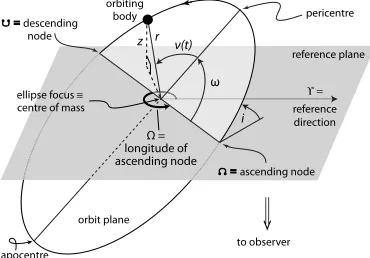
The inclination i, longitude of the ascending nodeΩ, and argument of pericenter

ω describe the projection of the three dimensional orbit onto the reference plane

tangent to the observer’s line of sight (the gray plane in Figure 1.3). We additionally

define the true anomaly ν(t) as the time-dependent angle describing the body’s

location on the ellipse, and z(t) as the body’s height on the ellipse relative to the

reference plane. Hence, z(t)describes the body’s motion along the observer’s line

of sight.

10 Radial velocities

Thetrue anomaly,ν(t), also frequently denotedf(t), is the angle between the direction of pericentre and the current position of the body measured from the barycentric focus of the ellipse. It is the angle normally used to characterise an observational orbit.

Theeccentric anomaly,E(t), is a corresponding an-gle which is referred to theauxiliary circleof the ellipse. The true and eccentric anomalies are geometrically re-lated by

cosν(t)=₁cosE(t)−e

−ecosE(t), (2.6)

or, equivalently,

tanν(t)

2 =

!₁

+e

1−e

"1/2

tanE(t)

2 . (2.7)

Themean anomaly,M(t), is an angle related to a fictitious mean motion around the orbit, used in calcu-lating the true anomaly. Over a complete orbit, during which the real planet (or the real star) does not move at a constant angular rate, an average angular rate can nev-ertheless be specified in terms of themean motion

n≡2π/P, (2.8)

wherePis the orbital period. The mean anomaly at time

t−tpafter pericentre passage is then defined as

M(t)=2_Pπ(t−tp)≡n(t−tp) . (2.9)

The relation between the mean anomaly,M(t), and the eccentric anomaly,E(t), can be derived from orbital dy-namics. This relation, Kepler’s equation, is given by

M(t)=E(t)−esinE(t) . (2.10) The position of an object along its orbit at any cho-sen time can then be obtained by calculating the mean anomalyMat that time from Equation 2.9, (iteratively) solving the transcendental Equation 2.10 forE, and then using the geometrical identity Equation 2.6 to obtainν.

Orbit specification A Keplerian orbit in three

dimen-sions (Figure 2.2) is described by seven parameters:

a,e,P,tp,i,Ω,ω. The first two,aande, specify the size and shape of the elliptical orbit.Pis related toaand the component masses through Kepler’s third law (see be-low), whiletpcorresponds to the position of the object

along its orbit at a particular reference time, generally with respect to a specified pericentre passage.3

The three angles (i,Ω,ω) represent the projection of the true orbit into the observed (apparent) orbit; they

3_{A few remarks are in order: (i) some texts state that just six} parameters are required, and omitP, implicitly invoking the re-lation betweenaandP(and the component masses) as given by Kepler’s third law; (ii)ais the semi-major axis of the orbit-ing body with respect to the system barycentre, assumed here

reference plane

ძ ascending node

i

orbit plane ν(t)

Ω = longitude of ascending node

ω _ϒ₌

reference direction

⇓

to observer orbiting body pericentre

ellipse focus ≡

centre of mass

r z წ descending

node

apocentre

Figure 2.2: An elliptical orbit in three dimensions. The reference plane is tangent to the celestial sphere.iis the inclination of the orbit plane. The nodes are the points where the orbit and ref-erence planes intersect.Ωdefines the longitude of the ascend-ing node, measured in the reference plane.ωis the fixed angle defining the object’s argument of pericentre relative to the as-cending node. The true anomaly,ν(t), is the time-dependent angle characterising the object’s position along the orbit.

depend solely on the orientation of the observer with re-spect to the orbit. In general, the semi-major axis of the true orbit does not project into the semi-major axis of the apparent orbit.

ispecifies theorbit inclinationwith respect to the reference plane, in the range 0≤i<180◦. i=0◦ cor-responds to a face-on orbit. In the discussion of binary orbits, motion is referred to as prograde (in the direc-tion of increasing posidirec-tion angle on the sky, irrespective of the relation between the rotation and orbit vectors) if

i<90◦, retrograde ifi>90◦, and projected onto the line of nodes ifi=90◦.

Ωspecifies thelongitude of the ascending node, mea-sured in the reference plane. It is the node where the measured object moves away from the observer through the plane of reference. [For solar system objects, it is the node where an orbiting object moves north through the plane of reference.]

ωspecifies theargument of pericentre, being the an-gular coordinate of the object’s pericentre relative to its ascending node, measured in the orbital plane and in the direction of motion. [Fore=0, where pericentre is undefined,ω=0 can be chosen such thattpgives the

time of nodal passage.]

to be in linear measure unless otherwise noted. Ifais deter-mined in angular measure, as in the relative astrometry of bi-nary stars, the system distanced(equivalently the parallaxϖ) is required to establish the linear scale; (iii) the parameters of the two co-orbiting bodies (e.g. a star and planet) with respect to the barycentre are identical, with the exception of their val-ues ofawhich differ by a factorMp/M⋆, and their values ofω

which differ by 180◦.

Figure 1.3: An illustration of a three dimensional Keplerian orbit. The labeled parameters are described in the main text. This figure is adopted from M. Perryman (2011).

Following M. Perryman (2011), if we consider Figure 1.3 to represent a star orbiting

the center of mass of the planet-star system, the star’s radial motionz(t)is given by

(22)

whered(t)is the star’s distance from the center of mass. Differentiating with respect

to time and simplifying the result gives the radial velocity of the star:

vr =K[_cos(ω+ν(t))+ecosω]. (1.3)

Here, K is the semi-amplitude of the star’s radial velocity. Substituting Kepler’s

laws gives a practical expression forK:

K = 28.4329 m s

−₁

√

1−e2

m2sini

MJup

m1+m2

M

−2/3 P

1 yr −1/3

, (1.4)

where m1 is the mass of the star, m2 is the mass of the planet, MJup is the mass

of Jupiter, and M is the mass of the Sun. Using Kepler’s third law, we can also express Equation 1.4 in terms of the planet’s semi-major axis:

K = 28.4329 m s

−₁

√

1−e2

m2sini

MJup

m1+m2

M

−1/2 _a

1 au −1/2

. (1.5)

A Jupiter-mass planet orbiting a solar-mass star at 5.0 au givesK = 12.7 m s−1, while an Earth-mass planet orbiting a solar-mass star at 1.0 au givesK =0.09 m s−1.

If the planet is assumed to be much less massive than the star, and the star’s mass is

known, then fitting an observed radial velocity curve to K and egives an estimate

of the planet’s minimum massm2sini.

In the late 19th and early 20th Century, RV measurements were routinely employed

to study stellar binaries and pulsations (Wilson, 1953). In 1952, University of

California, Berkeley, astronomer Otto Struve suggested that RV measurements could

be used to detect exoplanets. He wrote that "a planet might exist at a distance of

1/50 au ... causing the observed radial velocity of the star to oscillate with a range

of 0.2 km/s - a quantity that might be just detectable" (Struve, 1952). It was not until

1995, however, that the first unambiguously planetary-mass companion was detected

with the RV method: the 0.5MJupplanet orbiting the solar-type star 51 Pegasi b was

the first of the 1000+ planets now discovered with RVs (Mayor and Queloz, 1995).

While the radial velocity method continues to discover new exoplanets, its role as a

follow-up technique is increasing in importance. This role will be discussed further

in the transit method subsection below.

Figure 1.1 illustrates an important shortcoming of RV efforts to date: no planets

with masses less than or equal to that of the Earth have yet been detected with the

RV method. Detecting the radial velocity signals of such low-mass exoplanets is the

(23)

Additional Methods for Probing Exoplanet Masses

The radial velocity method is one among several techniques that are sensitive to

exoplanet masses. While these additional techniques will not be discussed further

in this thesis, they are briefly introduced below.

Figure 1.1 shows the ∼ 20 planets that have been detected with gravitational

mi-crolensing. When two distant stars align radially from the perspective of the Earth,

the gravitational influence of the foreground star bends the light of the background

star. To the Earth-bound observer, the background star appears to temporarily

brighten. For certain geometries, the gravity of a planet orbiting the foreground star

will further brighten the image of the background star for a fraction of the duration

of the full lensing event. These microlensing light curves can be used to reconstruct

that planet’s mass and orbital elements. The most important advantage of the

mi-crolensing technique is that it can detect planets at much larger distances from the

Earth than any other method of exoplanet detection. Because it is a photometric

technique, it is well-suited to monitoring many stars at one time. The principal

disadvantages of the technique are that the microlensing events are non-repeating,

and the planets it identifies cannot be followed up with other detection methods.

Exoplanets can also be detected by measuring the deflection of the parent star’s

position on the sky due to the gravitational influence of the planet. This astrometric

technique produced the first claims of exoplanet detections in the 1940s (e.g. Strand,

1943). Unfortunately, these and all subsequent claims have been refuted with

additional astrometric data and follow up with the radial velocity method. The

space-based Gaia astrometric monitoring mission, however, is expected to identify

tens of thousands of exoplanets by the end of its five-year mission (M. Perryman

et al., 2014).

The Transit Method

An exoplanet transit occurs when a planet crosses the line of sight between the

observer and the planet’s host star (Figure 1.4). The planet is detected as a diminution

of the starlight that recurs with the period of the planet’s orbit. Assuming that the

planet’s nightside contributes negligible flux to the star-planet system, a full transit

diminishes the starlight by the ratio of the planetary to stellar radii. In the infrared,

sufficiently warm planets can also be detected as they pass behind their parent stars:

during this “occultation” event, the total flux of the system is reduced as the planet’s

(24)

6

AA48CH16-Seager ARI 27 July 2010 15:21

Primary eclipse

Measure size of planet See star’s radiation transmitted through the planet atmosphere

Secondary eclipse

See planet thermal radiation disappear and reappear

Learn about atmospheric circulation from thermal phase curves

Figure 5

Schematic of a transiting exoplanet and potential follow-up measurements. Note that primary eclipse is also called a transit.

from direct imaging. The first event is the existence and discovery of a large population of planets orbiting very close to their host stars. These so-called hot Jupiters, hot Neptunes, and hot super Earths have up to about four-day orbits and semimajor axes less than 0.05 AU (seeFigure 1). The hot Jupiters are heated by their parent stars to temperatures of 1,000 to 2,000 K, making their IR brightness on the order of 1/1,000 that of their parent stars (Figure 4). Although it is by no means an easy task to observe a 1:1,000 planet-star flux contrast, such an observation is possible, and it is unequivocally more favorable than the 10−10_{visible-wavelength planet-star contrast for}

an Earth twin orbiting a Sun-like star.

The second favorable occurrence is that of transiting exoplanets—planets that pass in front of their star as seen from Earth. The closer the planet is to the parent star, the higher its probability to transit. Hence, the existence of short-period planets has enabled the discovery of many transiting exoplanets. It is the special transit configuration that allows us to observe the planet atmosphere without imaging the planet.

Transiting planets are observed in the combined light of the planet and star (Figure 5). As the planet passes in front of the star, the starlight drops by the amount of the planet-to-star area ratio. If the size of the star is known, the planet size can be determined. During transit, some of the starlight passes through the the planetary atmosphere (depicted by the annulus inFigure 5), picking up some of the spectral features in the planet atmosphere. A planetary transmission spec-trum can be obtained by dividing the specspec-trum of the star and planet during transit by the specspec-trum of the star alone (the latter taken before or after transit).

Planets on circular orbits that pass in front of the star also disappear behind the star. Just before the planet goes behind the star, the planet and star can be observed together. When the planet disappears behind the star, the total flux from the planet-star system drops because the planet no longer contributes. The drop is related to both the relative sizes of the planet and star and their relative brightnesses (at a given wavelength). The flux spectrum of the planet can be derived by subtracting the flux spectrum of the star alone (during secondary eclipse) from the flux spectrum of both the star and planet (just before and after secondary eclipse). The planet’s

www.annualreviews.org•Exoplanet Atmospheres 639

Annu. Rev. Astron. Astrophys. 2010.48:631-672. Downloaded from www.annualreviews.org Access provided by California Institute of Technology on 04/20/17. For personal use only.

Transit

Occultation

(a)

Phase Rela tiv e fl ux 0.98 0.99 1.00 1.01 a b 1.005 1.004 1.003 1.002 1.002 1.000 0.999

–0.1 0 0.1 0.2 0.3 0.4 0.5 0.6

Figure 6

Infrared light curve of HD 189733A and b at 8µm. The flux in this

light curve is from the star and planet combined. (a) The first dip (fromleft to right) is the transit and the second dip is the secondary eclipse. (b) A zoom in of panel

a. Error bars have been suppressed for clarity. Adapted from Knutson et al. (2007a).

flux gives information on the planetary atmospheric composition and temperature gradient (at IR wavelengths) or albedo (at visible wavelengths).

Observations of transiting planets provide direct measurements of the planet by separating photons in time, rather than in space as does imaging (seeFigures 5and6). That is, observations are made of the planet and star together. (We do not favor the combined light terminology because ultimately the photons from the planet and star must be separated in some way. For transits and eclipses, the photons are separated in time.) Primary and secondary eclipses enable high-contrast measurements because the precise on/off nature of the transit and secondary eclipse events provide an intrinsic calibration reference. This is one reason why the HST and theSpitzerhave been so successful in measuring high-contrast transit signals that were not considered in their designs.

2.2. Atmosphere Models and Theory

A range of models are used to predict and interpret exoplanet atmospheres. Usage of a hierar-chy of models is always recommended. Interpreting observations and explaining simple physical phenomena with the most basic model that captures the relevant physics often lends the most support to an interpretation argument. More detailed and complex models can further support results from the more basic models. The material in this subsection is taken from Seager (2010).

2.2.1. Computing a model spectrum.The equation of radiative transfer is the foundation not only to generating a theoretical spectrum but also to atmosphere theory and models. The radiative transfer equation is the change in a beam of intensitydI/dzthat is equal to losses from the beam –κIand gains to the beamε, and the 1D plane-parallel form is

µd I(z,ν, µ,t)

d z =−κ(z,ν,t)I(z,ν, µ,t)+ε(z,ν, µ,t).

Here,Iis the intensity [ Jm−2_s−1_Hz−1_{], a beam of traveling photons;}_κ_{is the absorption coefficient} [m−1_{], which includes both absorption and scattering out of the radiation beam;}_ε_{is the emission}

640 Seager

·

Deming

–0.1 0 0.1 0.2 0.3 0.4 0.5 0.6

Figure 6

Infrared light curve of HD 189733A and b at 8µm. The flux in this light curve is from the star and planet combined. (a) The first dip (fromleft to right) is the transit and the second dip is the secondary eclipse. (b) A zoom in of panel

µd I(z,ν, µ,t)

640 Seager

·

Deming

–0.1 0 0.1 0.2 0.3 0.4 0.5 0.6

Figure 6

Infrared light curve of HD 189733A and b at 8µm. The flux in this light curve is from the star and planet combined. (a) The first dip (fromleft to right) is the transit and the second dip is the secondary eclipse. (b) A zoom in of panel

µd I(z,ν, µ,t)

640 Seager

·

Deming

(b)

Figure 1.4: A schematic illustration of the transit method of exoplanet detection and atmospheric characterization. Panel (a) shows a cartoon of a transit event as a planet passes in front of its host star. This event corresponds to the first flux diminution in the plot of stellar flux versus planet phase in panel (b). The second, smaller diminution corresponds to the occultation event. This figure is adapted from S. Seager and Deming (2010).

Two years after the discovery of the first transiting exoplanet, D. Charbonneau,

Brown, et al. (2002) detected the first exoplanet atmosphere: using the Hubble Space

Telescope, the transit depth was observed to vary as a function of wavelength as the

planet’s atmosphere absorbed the starlight passing through it. Observations of planet

occultations in the mid-IR also give spectroscopic results: as the occultation’s depth

varies with wavelength, features in the planet’s thermal emission can be uncovered

(e.g. D. Charbonneau, Allen, et al. 2005 and Deming, S. Seager, Richardson, et al.

2005). The Transiting Exoplanet Survey Satellite (TESS) mission, scheduled for

launch in 2018, is designed to search for transiting exoplanets around bright stars –

these will be the most favorable planets for transmission and emission spectroscopy

studies in the future (Ricker, 2014).

The time between transits and occultations has also proven to be useful – Knutson

et al. (2007) observed the first flux variations as the warm dayside of the transiting

planet HD 189733 b rotated in and out of view. This “phase curve” measurement

gave insight into the transport of heat between the tidally locked planet’s perpetual

day and night sides, revealing a hot spot displaced from the nearest point to the star.

Because the brightness of many stars can be monitored simultaneously with modern

wide field imagers, the transit method is well suited to large-scale planet searches.

From 2009 to 2013, the Kepler space telescope continuously monitored a 115 deg2 region of the sky, identifying> 2300 transiting exoplanets (Borucki, D. Koch, et al.,

2010; Batalha, 2014). While the Kepler mission was not sensitive to planets with

(25)

extrapolated to conclude that 5.7+−1₂..7₂% of Sun-like stars have an Earth-radius planet

with an orbital period of 200−400 days (Petigura, A. W. Howard, and G. W. Marcy,

2013).

Since an observed transit ensures that the planet’s inclination is near zero, a detection

of the same planet with the radial velocity method yields a powerful combination:

the planet’s radius and mass, assuming that the host star’s mass and radius are also

known. The bulk density given by these two values allows planets to be classified as

gas giants (e.g. Jupiter), ice giants (e.g. Neptune), or rocky planets like the Earth.

Imaging

Direct imaging is perhaps the most intuitive method for exoplanet discovery and

characterization: by detecting an exoplanet as a separate point source from its host

star, the projected position and spectrum of the planet can be directly observed.

Because direct imaging is currently the only method for obtaining spectra of

non-transiting planets, its development is crucial to the success of the field – high

resolution spectroscopy is required to probe the compositions of planets and their

atmospheres. Furthermore, because the probability of transit decreases with the

planet’s semi-major axis, direct imaging is particularly useful for obtaining spectra

of exoplanets orbiting more than a few astronomical units from their host stars.

Direct imaging is challenging due to the combination of planets’ angular proximity

to their host stars and the typically small planet-to-star flux ratios. Following S.

Seager (2010), this flux ratio can be approximated as

fp(i, φ, λ)

fs(λ) = p

(λ)

R

p a

2

g(i, φ)+ Bλ

(T_eff_,_p)R2

p Bλ(Teff,s)R2s

. (1.6)

The first term on the right hand side of Equation 1.6 refers to the fraction of starlight

reflected by the planet, wherep(λ)is the geometric albedo of the planet as a function

of wavelength, Rpis the radius of the planet, a is the semi-major axis, andg(i, φ)

is the phase function. If the planet is approximated as a fully reflecting, diffusively

scattering sphere, p(λ) = 2/3. The phase functiong(i, φ)gives the fraction of the

planet’s disk that is illuminated by the star in terms of the orbital inclinationi and

the orbital phaseφ. The second term on the right hand side of Equation 1.6 gives the

relative contributions of the star and planet’s thermal radiations. Both objects are

approximated as blackbodies with specific intensitiesBλgiven by the Plank function

(26)

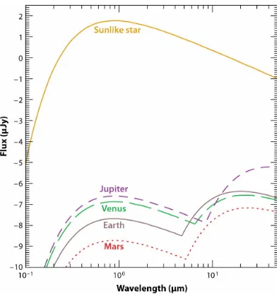
To illustrate these contributions to the planet-to-star flux ratio, Figure 1.5 shows the

flux of a solar system analog at a distance of 10 pc, where the Sun is approximated

as a Teff = 5750 K blackbody. The first hump in the maximum-phase planetary

fluxes is due to reflected starlight (see the first term in Equation 1.6), where the

reflected light flux ratio of the Earth-Sun analog reaches a maximum of about 10−10. The second hump is due to the planets’ thermal emission (see the second term in

[image:26.612.208.404.220.428.2]

Equation 1.6). The Earth-Sun analog’s flux ratio reaches a maximum of about 10−7 in the infrared.

Figure 1.5: The flux as a function of wavelength for a solar system analog at 10 pc. This figure is adapted from S. Seager and Deming (2010).

At a distance of 10 pc, a planet with a semi-major axis of 1 au would appear at an

angular separation of 0.100 from its parent star. Detecting such a planet is beyond the capabilities of current exoplanet imaging instruments. Section 1.2 explains the

practical challenges and opportunities for such instruments.

Within the purview of modern instrumentation, however, is the direct imaging of

young, massive planets located & 10 au from their parent stars (see the pink dots

on Figure 1.1). Unlike the∼ 4 Gyr Earth, whose infrared emission is dominated by

re-radiated starlight, planets in the first∼ 100 Myrs of their lives thermally radiate

their energy of formation and gravitational contraction.

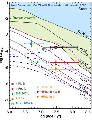
Figure 1.6 plots models of the luminosity versus age of low mass stars, brown

dwarfs, and planets of various masses, with several directly imaged planets and

(27)

that their luminosity at 1 Myrs is more than an order of magnitude greater than

their luminosity at 100 Myrs, emphasizing the advantageousness of young, massive

planets for direct imaging studies. Indeed, the planet-to-star flux ratio of the directly

imaged planet βPictoris b (gray point on Figure 1.6) is 10−4at 2.18µm (Bonnefoy, Lagrange, et al., 2011). _{M. Bonnefoy et al.: Characterization of the gaseous companion}__{Andromedae b}

6.0 6.5 7.0 7.5 8.0 8.5

log (age) [yr] -7 -6 -5 -4 -3 -2 -1 log L/L Sun

6.0 6.5 7.0 7.5 8.0 8.5

log (age) [yr] -7 -6 -5 -4 -3 -2 -1 log L/L Sun Brown dwarfs Stars 3 M Jup 5 M Jup 10 M Jup 13.6 M Jup 30 M Jup 78 M Jup HR8799 b

HR8799 c & d

HR8799 e

β Pic b

2M1207 b AB Pic b

1RXS1609 b

κ And b

Fig. 10. Evolution of the luminosity of gaseous objects

pre-dicted by the COND models (black solid line), and Marleau & Cumming (2013) models with typical “hot-start” (light pink dashed curve; 3, 5, 10, 13.6 MJup), and “cold-start” initial condi-tions (dark blue dashed curve; 3, 5, 10, 13.6 MJup). We over-lay measured luminosity of young low mass companions. A more complete version of this figure can be found in Marleau & Cumming (2013).

We also derived absolute flux predictions of SB12 models for the given filter passbands and the four sets of boundary conditions (free models at solar metallicity - cf1s, cloud-free models with three times the solar metallicity - cf3s, hybrid clouds at solar metallicity - hy1s, hybrid clouds with three times

the solar metallicity - hy3s) used forAnd b following the same

method as in Bonnefoy et al. (2013a). These synthetic fluxes were compared to the observed SED. The results are reported in Table 5. The comparison is biased by the limited mass coverage of the models. We note however, that solutions found within the models boundaries correspond to initial entropies intermediate between those of hot and cold-start models, placing the mass at

the typical planet/brown-dwarf boundary (⇠13.6MJupSpiegel

et al. 2011b; Molli`ere & Mordasini 2012; Bodenheimer et al.

2013). These solutions correspond to Te↵values that are in good

agreement with those determined from the companion SED.

In comparison, the models of Marleau & Cumming (2013) have a much simpler outer boundary condition (hereafter MC13), using a grey, solar-metallicity atmosphere. We used them as they can be used to evaluate the impact of underly-ing hypotheses made in the models (e.g. atmosphere treatment,

equation of state) on the derived joint mass and Sinitvalues. We

[image:27.612.217.396.178.412.2]

ran Markov Chain Monte Carlo simulations (MCMCs) in mass and initial entropy as in Marleau & Cumming (2013) with the related models to account for the uncertainties on the age, Te↵,

Table 5.Best fit photometric predictions of the “warm-start”

evolutionary models. Solutions found at the edges of the param-eter space (mass, Sinit) covered by the models are highlighted in italic.

Atmospheric model Age Mass Sinit 2 (Myr) (MJup) (kB/baryon) Cloud free - 1x solar 20 15 9.75 83.19 Cloud free - 3x solar 20 15 9.75 57.77 Hybrid cloud - 1x solar 20 14 9.75 14.56 Hybrid cloud - 3x solar 20 14 9.75 11.92 Cloud free - 1x solar 30 14 9.75 83.39 Cloud free - 3x solar 30 14 9.75 58.32 Hybrid cloud - 1x solar 30 14 10.25 13.73 Hybrid cloud - 3x solar 30 14 10.00 11.29 Cloud free - 1x solar 50 14 10.25 82.45 Cloud free - 3x solar 50 14 10.50 57.66 Hybrid cloud - 1x solar 50 14 13.00 19.30 Hybrid cloud - 3x solar 50 14 13.00 16.27 Cloud free - 1x solar 150 14 13.00 185.43 Cloud free - 3x solar 150 14 12.75 175.71 Hybrid cloud - 1x solar 150 14 13.00 173.50 Hybrid cloud - 3x solar 150 14 13.00 168.67

0 2 4 6 8 10 12 14

Mass [MJup] 8 9 10 11 12 13

Initial entropy [k

B

/baryon]

0 2 4 6 8 10 12 14

Mass [MJup] 8 9 10 11 12 13

Initial entropy [k

B

/baryon]

0 2 4 6 8 10 12 14

8 9 10 11 12 13

Initial entropy [k

B

/baryon]

0 2 4 6 8 10 12 14

Mass [MJup] 8 9 10 11 12 13

Initial entropy [k

B

/baryon]

0 2 4 6 8 10 12 14

Mass [MJup] 8 9 10 11 12 13

Initial entropy [k

B

/baryon]

0 2 4 6 8 10 12 14

8 9 10 11 12 13

Initial entropy [k

B /baryon] L/LSun Teff Upper limit Lower limit Estimate

Fig. 11.Predictions of the “warm-start” evolutionary models of

SB12 forAnd b for a system att⇡30+20

10Myr. The extreme

val-ues of the companion age, Te↵, and luminosities define a range

of masses and initial entropies lying between the dashed and dotted-dashed curves. We also overlay the initial entropies con-sidered in “hot-start” (open circles) and “cold-start” (dots) mod-els of FM08 (based on Marley et al. 2007).

and luminosity ofAnd b. We assumed Gaussian distributions

onLand Te↵. We took normal or lognormal errorbars for the two

considered age ranges (t=30+20

10Myr andt=30+12010 Myr), and chose flat priors inSinitandM.

Fig. 12 displays the 68-, 95- and 99 % joint confidence re-gions from the MCMC runs for both age groups. Open and closed circles are as in Marley et al. (2007), show the approx-imate range of entropies spanned by hot and coldest starts, re-spectively, but shifted upwards by+0.38kB/baryon to match the

12

Figure 1.6: The luminosity of stars, brown dwarfs, and planets are plotted as a function of age. Several directly imaged exoplanets are overplotted. This figure is adapted from Bonnefoy, Currie, et al. (2014).

Figure 1.6 also illustrates several important questions raised by the discovery of

∼ _{10 M}_Jup _{substellar companions – namely, how these bodies formed, and what,}

if anything, distinguishes them from brown dwarfs. A simplistic division between

brown dwarfs and giant planets is the 13 MJupmass cutoff for deuterium burning: in

the absence of nuclear fusion at any point during its lifetime, perhaps a companion

body could safely be called a planet. However, this demarcation was called into

question with the discovery of the first directly imaged M < 13 MJup companion:

2M1207–3932 b is a∼ 5 MJup object at a distance of 41 au from a 25 MJup brown

dwarf (Chauvin et al., 2004). While the lower mass companion certainly falls below

the deuterium burning mass limit, the two bodies are similar enough in mass that

they are likely to have formed like a binary star system via cloud fragmentation.

Hence, a more robust division between planets and brown dwarfs may be their

A Toolbox for Exoplanet Exploration

Rebecca Jensen-Clem

ACKNOWLEDGEMENTS

ABSTRACT

PUBLISHED CONTENT AND CONTRIBUTIONS

TABLE OF CONTENTS

LIST OF ILLUSTRATIONS

LIST OF TABLES

INTRODUCTION

⇓

·

·

·