www.hydrol-earth-syst-sci.net/18/343/2014/ doi:10.5194/hess-18-343-2014
© Author(s) 2014. CC Attribution 3.0 License.
Hydrology and
Earth System
Sciences
Data-driven scale extrapolation: estimating yearly discharge for a
large region by small sub-basins
L. Gong
Department of Earth Sciences, Uppsala University, Uppsala, Sweden Correspondence to: L. Gong ([email protected])
Received: 29 March 2012 – Published in Hydrol. Earth Syst. Sci. Discuss.: 1 June 2012 Revised: 30 October 2013 – Accepted: 6 December 2013 – Published: 28 January 2014
Abstract. Large-scale hydrological models and land surface
models are so far the only tools for assessing current and fu-ture water resources. Those models estimate discharge with large uncertainties, due to the complex interaction between climate and hydrology, the limited availability and quality of data, as well as model uncertainties. A new purely data-driven scale-extrapolation method to estimate discharge for a large region solely from selected small sub-basins, which are typically 1–2 orders of magnitude smaller than the large region, is proposed. Those small sub-basins contain suffi-cient information, not only on climate and land surface, but also on hydrological characteristics for the large basin. In the Baltic Sea drainage basin, best discharge estimation for the gauged area was achieved with sub-basins that cover 5 % of the gauged area. There exist multiple sets of sub-basins whose climate and hydrology resemble those of the gauged area equally well. Those multiple sets estimate annual dis-charge for the gauged area consistently well with 6 % av-erage error. The scale-extrapolation method is completely data-driven; therefore it does not force any modelling error into the prediction. The multiple predictions are expected to bracket the inherent variations and uncertainties of the cli-mate and hydrology of the basin.
1 Introduction
The interests in understanding current and future water re-sources have driven the rapid development of large-scale hy-drological models (e.g. Arnell, 1999, 2003, 2004; Vörös-marty et al., 1989, 2000a, 2004). Water resource projec-tions made by those models are an important basis for socio-economical analyses and decision-making processes (e.g.
Vörösmarty et al., 2000a). Projections of water resources are believed to be associated with large uncertainty, especially in ungauged basins that cover around 50 % of the global land area. For instance, global runoff estimates from various models differ between 29 000 km3yr−1and 43 000 km3yr−1 (i.e. around 30 %), and continental estimates differ up to 70 % (Widén-Nilsson et al., 2007). Besides climate and dis-charge data uncertainties, model uncertainties also signifi-cantly contribute to the uncertainties of the simulated dis-charge (Widén-Nilsson et al., 2009). A number of regional-isation methods have been developed to extend the predic-tion capability of hydrological models into ungauged areas. Commonly used regionalisation methods utilise spatial prox-imity and catchment similarity to transfer model parameters from gauged to ungauged basins (e.g. Kokkonen et al., 2003; Huang et al., 2003; Xu 1999, 2003; Kim and Kaluarachchi, 2008; McIntyre et al., 2005). Model averaging (i.e. using average of model outputs from different proximity or simi-larity approaches) was found to provide more robust results in regionalisation (e.g. McIntyre et al., 2005). Hydrological models inherently have limited parameter transferability over different spatial scales; therefore large-scale regionalisation methods use large gauged river basins as potential donors. However, averaged basin characteristics often cannot suffi-ciently summarise small-scale variability and nonlinearity, which might limit the prediction accuracy of the regionali-sation methods.
and annual runoff variability are governed, to the first order, by the relative availability of water and energy, while topog-raphy, basin storage and biological processes modulate these effects (Blöschl et al., 2013). It has long been recognised that the interaction between climate and hydrology controls the nonlinear partitioning of precipitation (e.g. L’vovich, 1979; Budyko, 1974; Wagener et al., 2007). L’vovich (1979) and Budyko (1974) were among the first to characterise climate and hydrology using long-term average water and energy bal-ance variables. The aridity index, as expressed by the ratio of long-term average potential evapotranspiration to that of pre-cipitation, has long been used as a useful index describing the interaction between climate and hydrology of a region (e.g. Wagener et al., 2007). Interestingly, a number of simi-larity studies have shown that climate has a universal control over hydrology for basins over a wide range of spatial scales, i.e. from 10 to 10 000 km2(Troch et al., 2009; Voepel et al., 2011; Brooks et al., 2011). The scale independence of hy-drological similarity indicates that small gauged basins can potentially be used as predictors for large-scale hydrological responses, provided that the small basins and the large region are similar in their essential climatic and hydrological param-eters. In contrast to regionalisation methods, this paper uses the similarity of climate time series as the foundation for ex-trapolation, instead of using similarity index and regression-based methods. This paper aims at developing a systematic methodology that allows discharge data of small basins to be extrapolated to a much larger scale. The main purpose of the paper is to present the methodology of scale extrapolation; however, we also showed how the method worked in one test basin (the Baltic Sea basin) with the preliminary results.
2 Study area and data
3 The Baltic Sea drainage basin
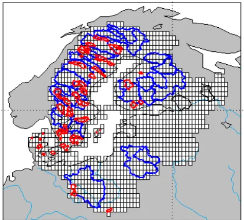
The extrapolation method was tested in the Baltic Sea drainage basin (Fig. 1). The Baltic Sea is one of the largest brackish seas in the world; the Baltic Sea drainage basin lies between maritime temperate and continental subarctic cli-mate zones. With a surface area of 415 000 km2, the drainage basin spans 14 countries with 85 million inhabitants, a ma-jority of them living in big cities. The Baltic Sea is semi-enclosed and therefore vulnerable to pollution, and its envi-ronmental status is one of the major concerns for the northern European countries. The Baltic Sea is affected by pollution from various sources including nutrient input from rivers, pollution from industries, and direct atmospheric depositions (Wulff et al., 2001). Many of these factors are dependent on the climate and hydrology in the basin.
17
1
[image:2.595.309.547.65.279.2]2
Figure 1. Map of the Baltic Sea drainage basin as shown by 0.5 degree STN-30p global grid 3
cells, with boundaries of 100 gauged-sub-basins shown by lines. Source-sub-basins are 4
marked with red and the rest marked with blue. 5
6
Fig. 1. Map of the Baltic Sea drainage basin as shown by 0.5
de-gree STN-30p global grid cells, with boundaries of 100 gauged sub-basins shown by lines. Source sub-sub-basins are marked with red and the rest marked with blue.
4 Data sets
Monthly precipitation for the period of 1975–2001 was taken from the 30-minute monthly Climatic Research Unit Time-Series (CRU TS) 2.1 database (Mitchell and Jones, 2005). The number of stations used by the CRU TS 2.1 data set has significant temporal variations (Mitchell and Jones, 2005). Spatial density of CRU precipitation stations in the Baltic Sea drainage basin decreased after 1990. Monthly precipi-tation data from 1984 SMHI (Swedish Meteorological and Hydrological Institute) precipitation stations for the period of 1961–2002 were interpolated to a regular 30 min grid, and the quality of the CRU precipitation data within Sweden was validated against the SMHI data prior to the analysis. The re-sults (figure not shown) showed that the spatial differences between CRU and SMHI annual average precipitation were similar for the period of 1961–1990 and 1991–2002. Dif-ferences between 1991–2002 and 1961–1990 mean annual precipitation as calculated by CRU data and SMHI data also agreed well in their general spatial pattern, although those calculated with SMHI data showed much higher spatial vari-ability at smaller scales.
downward short-wave radiation and net long-wave radia-tion were used to calculate reference evaporaradia-tion using the Penman–Monteith FAO-56 equation (Allen et al., 1998). Specific humidity was first converted to relative humidity us-ing a mixus-ing-ratio method, and 10 m wind speed was con-verted to 2 m wind speed using a logarithmic relationship (Allen et al., 1998). Prior to the calculation of reference evap-oration, the quality of the WFD air temperature, wind speed, and WFD-derived relative humidity was tested in a compar-ison with daily weather data (Global Surface Summary of the Day, or GSOD) from the National Climatic Data Center (NCDC, 2011). In the Penman–Monteith FAO-56 equation, surface albedo is fixed at 0.23; however we found this value is too high for the Baltic Sea basin. Therefore, the albedo values were taken directly from the ERA-Interim data set (Simmons et al., 2007). The daily WATCH forcing data were aggregated to obtain yearly values (calendar year) for each 30 min grid cell. The monthly CRU precipitation data were also aggre-gated to yearly values.
STN-30P data set (Vörösmarty et al., 2000b) was used to identify 1386 cells on a regular 30 min global grid that belong to the Baltic Sea drainage basin. HYDRO1k (USGS, 1996) was used to delineate the upstream area of the discharge sta-tions. The discharge data were taken from the Global Runoff Data Centre database (GRDC, 2012) and the SMHI Vatten Web (http://vattenweb.smhi.se/). Among 425 available sub-basins, 100 sub-basins were selected under the following cri-teria: (1) they do not contain nested sub-basins; (2) when reg-istered in the Hydro1k river network, the register area does not differ by more than 20 % with the reported area from GRDC or SMHI; and (3) they have complete daily data cov-erage from 1975 to 2001. Figure 1a shows the location of the 100 sub-basins. The sizes of the sub-basins vary between 5 and 109 564 km2. The area covered with the 100 gauged sub-basins, denoted as “gauged basin area”, was used to val-idate the scale-extrapolation method (Fig. 1). The success-fulness of the scale extrapolation depends on the abundance of discharge data from small river basins. For the extrapola-tion to perform well, it is critical to select river basins within a suitable size range. The resolution of the available global or regional climate data set defines the lower limit for the size of the small river basins that can be used for extrapola-tion (i.e. the size of a river basin should be comparable with the climate grid), so reliable climate data can be obtained for the basin. Preliminary results showed that river basins be-tween 500 and 5000 km2 are most useful for discharge ex-trapolation at the global scale, considering that the resolu-tion of most global climate data sets is 0.5 degree. Therefore, only 51 sub-basins between 500 and 5000 km2, denoted as “source sub-basins” (Fig. 1), were selected for discharge ex-trapolation.
5 Self-similarity in hydrological response
In this paper, hydrological similarity refers to two or more basins that share similar factors controlling the discharge dy-namics. The controlling factors may include basin size, to-pography, soil, vegetation, climate, geology, as well as fac-tors that can be derived directly from data, for instance runoff coefficients, and factors that can be derived with the help of modelling or data analysis techniques, for instance topo-graphic index, aridity index and Horton index.
What can be more similar to a basin than the basin itself? If an ungauged basin A (Fig. 4a) is identical in every hydro-logical controlling factor with a gauged basin B, then A shall have the same discharge as B. But it is virtually impossible to find such a identical gauged basin, especially if A is a large-scale basin.
Topography and river channel networks have long been known to be self-similar. Inside a river basin one can always find a sub-region with similar topographic and channel net-work features. However, if discharge is to be extrapolated from a sub-region to the whole basin, all first-order control-ling factors of the sub-region should be self-similar to the basin. Therefore, there is a need to extend the self-similarity measures to include all important factors that control the hy-drological response.
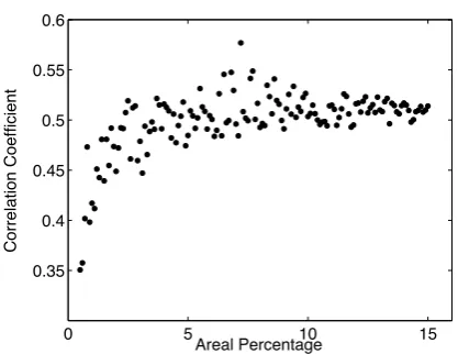
Each hydrological controlling factor, be it climate forcing or land surface parameters, exhibits spatial auto-correlation. Part of the spatial information is repetitive or redundant; there is only a limited number of unique patterns that de-fine the hydrological dynamics of a basin. Those patterns can be time series of climate forcing, or spatial statistics of a land surface parameter. For instance, when a number of cells within the gauged area of the Baltic Sea drainage basin was selected by the criterion that they must well resemble the temporal variation of yearly precipitation of the gauged area, the average correlation among those cells dropped sig-nificantly if less than 5 % of the cells were selected (Fig. 2). If more cells were selected, there would be significant corre-lation among the cells so that the addition of new cells may be redundant (Fig. 2).
18 1
2
Figure 2. Correlation coefficients (Y-axis) between annual precipitation time series of
3
selected cells from the source-sub-basins, as a function of the areal ratio between selected
4
cells and the gauged area of Baltic Sea drainage Basin (X-axis).
5 6
0 5 10 15
0.35 0.4 0.45 0.5 0.55 0.6
Areal Percentage
Correlation Coefficient
Fig. 2. Correlation coefficients (yaxis) between annual precipita-tion time series of selected cells from the source sub-basins, as a function of the areal ratio of selected cells to the gauged area of Baltic Sea drainage basin (xaxis).
1. Use only small (in the context of global hydrology) sub-basins. Both climate and hydrology exhibit larger spatial and temporal variability at smaller scales. A large spectrum of climate and land surface patterns can be obtained by combining several small basins. 2. Allow partial selections of cells within each source
sub-basin. Therefore, a source sub-basin can con-tribute any number of cells (from zero to its total num-ber of cells) to the final selected source cells. This strategy not only greatly increases the chance of a good “factor matching”, but also opens up the possibility of having a vast number of equally good realisations of source cells (i.e. different groups of cells that are hydrologically similar to each other and to the large basin).
A simple two-step test is made to illustrate the importance to allow the source cells to be spatially discrete. In step one, each source sub-basin alone was selected as a candi-date to represent the yearly discharge time series of a gauged area. A number of hydrological controlling factors, including yearly, monthly and average monthly (climatology) precipi-tation and potential evaporation, and the frequency distribu-tion of topographic index were calculated for both the source sub-basins and the gauged area. The degree of similarity of those factors was calculated by the standardised RMSE (root-mean-square error) values (SRMSE) as follows:
SRMSE=1 ¯
x·
v u u u t
n
P
i=1
xi0−xi
2
n , (1)
wherexistands for the time series of a controlling factor (e.g.
precipitation) of the entire gauged area, andxi0 stands for the time series of the same controlling factor for a single source
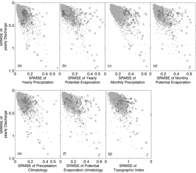
sub-basin. A smaller SRMSE value indicates more similarity. Similarly, the SRMSE values of yearly discharge were also calculated, and plotted against the SRMSE of each control-ling factor in Fig. 3a–g as black circles. The number of black circles corresponds to the number of source sub-basins. In step two, the source sub-basins were allowed to be randomly combined, and the combined area was used instead of a sin-gle sub-basin to represent the yearly discharge of the gauged area. A total of 10 000 such randomly combined areas were obtained. Their similarities in terms of hydrological control-ling factors and discharge with the entire gauged area were also calculated by SRMSE values and are plotted by grey dots in Fig. 3a–g.
Figure 3 shows that all controlling factors have significant control over the similarity of the discharge dynamics. For in-stance, if a source sub-basin or a combined area has simi-lar precipitation dynamics as the gauged area, its discharge is more likely to well resemble the discharge of the gauged area. On the other hand, a large deviation in any of the con-trolling factors is likely to mean poor discharge resemblance. Figure 3 also shows the limited ability of individual source sub-basins to capture the variation of any controlling factor of the gauged area. Combined source sub-basins can achieve much better resemblance for all controlling factors, and as they do so, they also better resemble the discharge dynamics of the gauged area.
Many controlling factors in Fig. 3 are correlated with each other; therefore, a multiple regression analysis was per-formed in order to identify the first-order controlling factors. Firstly a regression was made with the SRMSE of discharge as an independent variable and SRMSE of all controlling fac-tors as dependent variables. The result showed that the best linear combination of the dependent variables was able to explain 84 % of the variations of the independent variable. If only SRMSE values of yearly precipitation and potential evaporation were used as dependent variables, they would be able to explain 82 % of the variations of the independent vari-able. Although the addition of topographic index as a depen-dent variable can increase the degree of explanation (i.e. 1 % more of the variation of the dependent variable), in this paper only yearly precipitation and potential evaporation were used as first-order controlling factors for yearly discharge.
6 Data-driven scale extrapolation
Scale extrapolation is defined as the extrapolation of hydro-logical parameters (e.g. discharge) from small to large scale. We denote the collection of hydrological controlling factors
asX, so that
X= {x1, x2, . . . xn,}, (2)
wherex1, x2, . . . , xn are individual controlling factors. The
discharge, if not measured, can be estimated byX, such as
ˆ
[image:4.595.63.272.60.221.2]Fig. 3. The standardised root-mean-square error (SRMSE) of yearly discharge (1975–2001) calculated between sub-sets of the gauged area
and the gauged area itself (yaxis), plotted against SRMSE of seven hydrological controlling factors also calculated between subsets of the gauged area and the gauged area itself. Sub-sets were selected in two different ways: (1) by using individual source sub-basin alone (black circles) and (2) by randomly combing source sub-basins (grey dots). The seven hydrological controlling factors are yearly precipitation (a) and potential evaporation (b), monthly precipitation (c) and potential evaporation (d), precipitation (e), and potential evaporation climatology
(f) and the frequency distribution of topographic index (g).
Figure 4a illustrates an ungauged basin A and three of its source sub-basins,S1,S2andS3, which have discharge data D1,D2andD3, respectively. Inside each sub-basin, a group of cells (C1,C2andC3)is selected according to the follow-ing two criteria:
1. Inside each source sub-basin, a group of cells is se-lected so that it can resemble the yearly precipitation and potential evaporation of the sub-basin, such that
XCi≈XSi, i=1,2,3, (4)
whereXCandXSare the hydrological controlling
fac-tors for a cell group and for a source sub-basin, re-spectively. Therefore, it can be assumed that the cell group has the same discharge dynamics as the sub-basin (Fig. 4b), such that
ˆ
DCi≈DSi, i=1,2,3. (5)
2. The combination of all cell groups (i.e. the source cells) shall resemble the yearly precipitation and po-tential evaporation of the whole basin, such that
X(C1+C2+C3)≈XA. (6)
Therefore, the area-weighted average discharge from the source cells can be used to estimate the discharge of the whole basin (Fig. 4c), such that
ˆ
DA≈
ˆ
DC1 DˆC2 DˆC3
×
aC1 aC2 aC3
0
3
P
i=1
aCi
≈DS1 DS2 DS3
× [aC1 aC2 aC3]
0
3
P
i=1
aCi
20 1
(a)
2
3
4
(b)
5
6
7
(c)
[image:6.595.54.286.55.450.2]8
Figure 4. Schematic illustration of the scale-extrapolation method.
9
4(a): An un-gauged large basin A and its gauged sub-basins S1, S2 and S3, each contains a 10
group of cell C1, C2 and C3 respectively. 11
4(b): Cell groups C1, C2 and C3 can well resemble essential climate variables of their
12
respective sub-basins; therefore, C1, C2 and C3 are expected to have same discharge dynamic
13
as their respective sub-basins.
14
4(c): The combination of all cell groups can well resemble essential climate variables of basin
15
A; therefore, area-weighted discharge from all cell groups can be used to estimate the
16
discharge of basin A.
17
Fig. 4. Schematic illustration of the scale-extrapolation method. (a) An ungauged large basin A and its gauged sub-basinsS1,S2
andS3, each containing a group of cellC1,C2andC3, respectively.
(b) Cell groupsC1,C2andC3can well resemble essential climate variables of their respective sub-basins; therefore,C1,C2andC3
are expected to have same discharge dynamics as their respective sub-basins. (c) The combination of all cell groups can well resem-ble essential climate variaresem-bles of basin A; therefore, area-weighted discharge from all cell groups can be used to estimate the discharge of basin A.
whereaCi is the area of the cell groupCi. It is impor-tant to note that basin A can have more than three source sub-basins, and it is not necessary that all source sub-basins should contribute to source cells. If a source cell is on the border of a sub-basin, only the overlapping area is used in the area weighting. In this paper, we tested the scale-extrapolation method in the gauged basin area, formed by the 100 gauged sub-basins of the Baltic Sea drainage basin. 51 gauged sub-basins between 500 and 5000 km2were selected as source sub-basins. Monte Carlo method was used to select
21
1
(a) (b) 2
[image:6.595.311.547.65.290.2]3
Figure 5. 4
SRMSE values of yearly precipitation (a) and potential evaporation (b) plotted against 5
SRMSE values of yearly discharge, for 196 realisations of selected source cells with
6
discharge SRMSE values less than 0.1. Dashed lines indicate mean values.
7
Fig. 5. SRMSE values of yearly precipitation (a) and potential
evap-oration (b) plotted against SRMSE values of yearly discharge, for 196 realisations of selected source cells with discharge SRMSE val-ues less than 0.1. Dashed lines indicate mean valval-ues.
200 realisations of source cells (i.e. 200 different groups of cells that fulfil the above criteria). Each realisation of source cells was selected so that the SRMSE values for precipita-tion and potential evaporaprecipita-tion do not exceed threshold val-ues 3.5 % and 1.75 % respectively. The threshold value was selected to ensure that (1) there is a good resemblance of cli-mate time series between selected cells and the gauged basin area and (2) a sufficient number of different cell groups can be found to equally well resemble the gauged basin area. The threshold value can be region-dependent, and it should be a function of data quality and the spatial variability of regional climate. A total of 200 area-weighted discharge time series from the 200 realisations of source cells were then derived, and their similarity with the discharge of the entire gauged area was examined by calculating the SRMSE value.
7 Result
All 200 realisations of source cells closely resemble the yearly dynamics of precipitation and potential evaporation of the gauged area with very small SRMSE values (Fig. 5). The average SRMSE for precipitation is 3.1 % with a stan-dard deviation of 0.2 %. The average SRMSE for potential evaporation is 1.5 % with a standard deviation of 0.1 %. The average SRMSE for the 200 extrapolated yearly discharge time series is 6 % with a standard deviation of 1 %.
22 1
2
Figure 6. Quality of discharge extrapolation measured by SRMSE of yearly discharge 3
between gauged basin area and selected source-cells, plotted against areal ratio of selected 4
source-cells to the entire gauged basin area. Two different source-cell selection methods are 5
plotted: 1) randomly combining source-sub-basins (black) and 2) using the scale-6
extrapolation method, i.e., allowing a sub-set of a sub-basin to be selected (red). 7
8
0 5 10 15 20 25 30
0 0.05 0.1 0.15 0.2 0.25 0.3 0.35 0.4 0.45 0.5
Area percentage (%)
SRMSE of yearly discharge
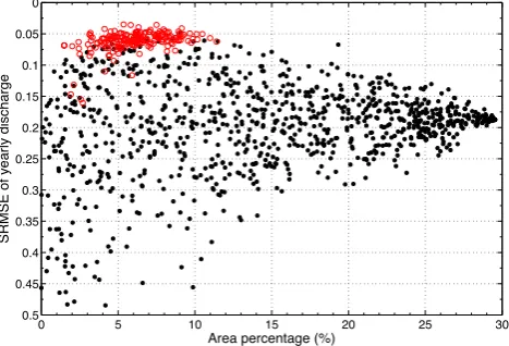
Fig. 6. Quality of discharge extrapolation measured by SRMSE of
yearly discharge between gauged basin area and selected source cells, plotted against areal ratio of selected source cells to the en-tire gauged basin area. Two different source-cell selection methods are plotted: (1) randomly combining source sub-basins (black) and (2) using the scale-extrapolation method, i.e. allowing a sub-set of a sub-basin to be selected (red).
of source cells to the entire gauged area. For the purpose of comparison, two different source-cell selection methods are plotted: (1) randomly selected source sub-basins were combined and all cells within each sub-basin were used to form the source cells; 1000 such combinations were used, and their SRMSE values were plotted as black dots; (2) the scale-extrapolation method was used (i.e. allowing a sub-set of a source sub-basin to be selected). The SRMSE values of 200 realisations of selected source cells were plotted as red circles. Figure 6 shows that most realisations of source cells selected by the scale-extrapolation method have the area ra-tio between 3 % and 10 %. With such area percentages it is most probable to find a good match of climate dynamics with the gauged area. Figure 6 also shows that the area ratio of the source cells to the whole gauged area plays an important control over the extrapolation quality. It seems that when the source cells are around 5 % of the entire gauged area, there is the best chance for a good extrapolation. The largest extrap-olation error occurred when the area ratio was too small.
Figure 7a and b show two examples of totally different realisations of selected source sub-basins (blue boundaries) and source cells (red). In the first example, the selected sub-basins represent precipitation and potential evaporation of the whole basin area with SRMSE values of 3.5 % and 2 % respectively (Fig. 8a and b); the extrapolated discharge well resembles discharge of the gauged area with SRMSE of 6 % (Fig. 9a). In the second example, precipitation and potential evaporation of the gauged area are represented with SRMSE values of 3.3 % and 2.6 % respectively (Fig. 8c and d), and the extrapolated discharge resembles discharge for the whole basins also with an SRMSE of 6 % (Fig. 9b).
23
1
2
(a) (b)
3
Figure 7a,b: Map of the Baltic Sea drainage basin as shown by 0.5 degree STN-30p global
4
grid cells, with two exampes of the selected source-basins and selected source-cells for the
5
discharge extrapolation in the Baltic Sea drainage basin.
6
Fig. 7. (a, b) Map of the Baltic Sea drainage basin as shown by
0.5 degree STN-30p global grid cells, with two examples of the selected source basins and selected source cells for the discharge extrapolation in the Baltic Sea drainage basin.
8 Discussions and conclusion
Small-scale dynamics can have a crucial impact on large-scale hydrological responses. A fundamental problem for large-scale hydrology is the difficulty in preserving the non-linearity at small scales. The superposition principle, appli-cable only for linear systems, states that the response caused by two or more inputs equals the sum of the responses, which would have been caused by each input individually. In terms of hydrology, this would imply that the hydrological response of a basin (or a grid cell), under distributed inputs, could be perfectly reproduced with spatially averaged inputs. This is not valid because hydrological systems are nonlinear, so that
f (X1)+f (X2)+. . .+f (Xn)
n 6=f (
X1+X2+. . .+Xn
n ), (8)
wherenis the number of response units (e.g. number of cells in a basin), and f (Xi) is the distributed hydrological
re-sponse under distributed hydrological controlling factor(Xi)
as defined in Sect. 4. Equation (8) has an interesting impli-cation: if two basins differ significantly in size, even if they share similar average hydrological controlling factors, they may have different discharge dynamics.
The result from this paper illustrates that it is impossible to use a single sub-basin or a single cell to represent the average dynamics of the gauged area of the Baltic Sea drainage basin. It is always necessary to use spatially discrete and scattered sub-regions to represent unique patterns of the hydrological controlling factors, even though the area of the sub-regions can be as small as 1.5 % of the gauged area. For the Baltic Sea drainage basin, a fairly accurate approximation can be achieved by relaxing Eq. (8), so that
f (X1)+f (X2)+. . .+f (Xn)
n
≈f
X
1+X2+. . .+Xm1 m1
[image:7.595.312.546.63.177.2] [image:7.595.52.286.68.227.2]24 1
(a) (b)
2
3
(c) (d)
[image:8.595.47.284.61.420.2]4
Figure 8. 5
8a,b: Yearly precipitation (a) and potential evaporation from (b) of the selected source-cells 6
(red) and of the entire gauged area (black) for example 1 (Figure 7a). 7
8c,d: Yearly precipitation (c) and potential evaporation from (d) of the selected source-cells 8
(red) and of the entire gauged area (black) for example 2 (Figure 7b). 9
1975 1985 1995
450 500 550 600 650 700 750 800
Year
mm/year
1975 1985 1995
310 320 330 340 350 360 370 380 390
Year
mm/year
1975 1985 1995
450 500 550 600 650 700 750 800
Year
mm/year
1975 1985 1995
290 300 310 320 330 340 350 360 370
Year
mm/year
Fig. 8. Yearly precipitation (a) and potential evaporation (b) of the
selected source cells (red) and of the entire gauged area (black) for example 1 (Fig. 7a). Yearly precipitation (c) and potential evapora-tion (d) of the selected source cells (red) and of the entire gauged area (black) for example 2 (Fig. 7b).
+f
Xm1+1+Xm1+2+. . .+Xm2 m2
+. . .
+f (Xmk+1+Xmk+2+. . .+Xn
mk ). (9)
Equation (9) categorises the n cells of a basin into k groups. Cells within each group have correlated controlling factors, and therefore may be considered quasi-linear, such that the hydrological response from a cell group can be well approximated by using an average input. Cell groups are, however, mutually independent of each other, and a mini-mal number of cell groups are needed to capture the variabil-ity of the whole basin. Equation (9) lends theoretical sup-port to the scale-extrapolation method. Precipitation time se-ries among selected source cells are mutually independent (Fig. 2), and each selected source sub-basin represents the average hydrological controlling factors for a certain region
25
1
(a) (b) 2
Figure 9. Yearly discharge from the gauged basin area (black) and extrapolated discharge 3
(red) using selected source-cells from example 1 (a) and example 2 (b). 4
5
1975 1980 1985 1990 1995 2000 150
200 250 300 350 400 450 500
Year
mm/year
1975 1980 1985 1990 1995 2000 150
200 250 300 350 400 450 500
Year
mm/year
Fig. 9. Yearly discharge from the gauged basin area (black) and
ex-trapolated discharge (red) using selected source cells from example 1 (a) and example 2 (b).
26
1
2
Figure 10. Sub-basins selected for inverse-extrapolation. The green-outlined small basin, with
3
an area of 2250 km
2, is found to have similar climate conditions as the selected cells (red,
4
21228 km
2in total) of two larger sub-basins.
5
6
Fig. 10. Sub-basins selected for inverse extrapolation. The
green-outlined small basin, with an area of 2250 km2, is found to have similar climate conditions as the selected cells (red, 21 228 km2in total) of two larger sub-basins.
within the gauged area, which can be regarded as quasi-linear in its hydrological dynamics.
Figure 6 showed that out of 200 realisations of the extrap-olated discharge, only 6 had SRMSE values of discharge of more than 10 %. Four of those relatively large extrapolation errors occurred when the area ratio of source cells to gauged area was too small (i.e. between 2 % and 3 %), while another two occurred when the area ratio was around 4 % and 6 %, respectively. This result further lends support to the fact that nonlinearity exists at large scale and even at yearly timescale. Although those small source-cell areas can perfectly resem-ble the average climate of the gauged area, they are unaresem-ble to resemble the discharge dynamics in a good way, because they do not cover the minimum number of unique patterns required in order to preserve the nonlinearity, as shown in Eq. (9).
[image:8.595.312.545.65.160.2] [image:8.595.312.542.228.441.2] [image:8.595.49.220.510.560.2]27 1
2
(a) (b) (c)
3 4
Figure 11. Values of yearly precipitation (a), potential evaporation (b) and discharge (c) of the 5
small sub-basin (green outlined in Figure 10), plotted by black lined; and a larger area (red 6
cells in Figure 10), plotted by red lines. 7
1975 1980 1985 1990 1995 2000
400 500 600 700 800 900 1000
Year
Precipitation (mm/year)
1975 1980 1985 1990 1995 2000
300 320 340 360 380 400 420
Year
Potential Evaporation
(mm/year)
1975 1980 1985 1990 1995 2000
100 200 300 400 500 600 700
Year
Discharge (mm/year)
Fig. 11. Values of yearly precipitation (a), potential evaporation (b) and discharge (c) of the small sub-basin (outlined in green in Fig. 10),
plotted by black lines, and a larger area (red cells in Fig. 10), plotted by red lines.
An inverse extrapolation was made to illustrate the existence of nonlinearity on a yearly timescale further. The inverse extrapolation, similar to the scale-extrapolation method, tries to match the hydrological controlling factors of a number of sub-basins to a single small sub-basin, instead of the large basin. A small sub-basin with a size of 2250 km2 (Fig. 10, outlined in green) was selected, and source cells (Fig. 10, red cells) from two other sub-basins (Fig. 10, blue outlined) with a total size of 21 228 (or 10 times bigger) were found to resemble the yearly precipitation and poten-tial evaporation of the small sub-basin well, with SRMSEs of 4.7 % and 2.6 % respectively (Fig. 11a and b). However, the discharge differs between the small basin and the larger region by 21 % (Fig. 11c). Of course, this is only one ex-ample, and more thorough tests should be made, preferably with climate data sets of higher resolution. The results of this paper showed that a minimum of 5 % of the basin area is needed to be able to account for the nonlinearity of the sys-tem; 5 %–10 % appears to be the area percentage for which the best extrapolation quality can be expected (Fig. 6). This percentage is expected to increase with finer timescales and to change with different climate and hydrological regimes.
A new data-driven scale-extrapolation method was pro-posed to estimate annual water resources for large river basins. The new method builds upon the fact that the dy-namic interaction between climate and hydrology of a large river basin can be equally well resembled by multiple small regions, each characterized by a number of small river basins that typically give around 5 % areal percentage of the large basin. Therefore, those multiple small regions can provide an ensemble of water resource estimations for the large basin. The new method, being purely data-based, makes it possi-ble for regional water resource estimations to benefit from a multitude of readily available measurements from small river basins.
The scale-extrapolation method provides both new methodology and new data into the field of large-scale hy-drology. It allows regional water resources to be estimated directly from small river basins that are typically 1–2 orders of magnitude smaller and therefore better preserve the small-scale dynamics and nonlinearity, which are vital for credible
predictions. The extrapolation is modelling-free, and there-fore the estimation is free of modelling uncertainties that usu-ally contribute significantly to large-scale estimation uncer-tainties. The method is not sensitive to the bias of the climate data set because the climate data set is only used for sub-basin selection and not directly for extrapolation.
The scale-extrapolation methods made it possible to study the interaction between climate and hydrology, and the cli-mate change impact in ungauged or partially gauged large river basins from data alone. At the same time, the method offers ensemble predictions that have the potential of brack-eting the estimation uncertainty. Because the scale extrapola-tion uses completely different data and method compared to the modelling approach, it provides a unique opportunity to be compared with modelling results.
Acknowledgements. This paper is funded by the Swedish Research
Council grant 621-2012-3903 and grant 214-2012-373 from the Swedish Research Council for Environment, Agriculture Sciences and Spatial Planning. Discharge data were provided by the Global Runoff Data Centre, 56068 Koblenz, Germany, and the Swedish Meteorological and Hydrological Institute. The author had dis-cussions with Fritjof Fagerlund and Anna Kauffeldt and received valuable insights.
Edited by: S. Thompson
References
Allen, R. G., Pereira, L. S., Raes, D., and Smith, M.: Crop evap-otranspiration – guidelines for computing crop water require-ments, FAO Irrigation and Drainge Paper, FAO, 1998.
Arnell, N. W.: A simple water balance model for the simulation of streamflow over a large geographic domain, J. Hydrol., 217, 314–335, 1999.
Arnell, N. W.: Effects of IPCC SRES* emissions scenarios on river runoff: a global perspective, Hydrol. Earth Syst. Sci., 7, 619–641, doi:10.5194/hess-7-619-2003, 2003.
[image:9.595.104.492.65.171.2]Blöschl, G., Sivapalan, M., Wagener, T., Viglione, A., and Savenije, H.: Runoff Prediction in Ungauged Basins: Synthesis Across Processes, Places and Scales, Cambridge University Press, 2013. Brooks, P. D., Troch, P. A., Durcik, M., Gallo, E., and Schlegel, M.: Quantifying regional scale ecosystem response to changes in precipitation: Not all rain is created equal, Water Resour. Res., 47, W00J08, doi:10.1029/2010WR009762, 2011.
Budyko, M. I.: Climate and life, New York, Academic Press, 508 pp., 1974.
GRDC: Global Runoff Data Centre, Global Runoff Data Centre, available at: http://grdc.bafg.de (last access: 15 October 2013), 2012.
Huang, M., Liang, X., and Liang, Y.: A transferability study of model parameters for the variable infiltration capac-ity land surface scheme, J. Geophys. Res., 108, 8864, doi:10.1029/2003JD003676, 2003.
Kim, U. and Kaluarachchi, J. J.: Application of parameter estima-tion and regionalizaestima-tion methodologies to ungauged basins of the Upper Blue Nile River Basin, Ethiopia, J. Hydrol., 362, 39–56, 2008.
Kokkonen, T. S., Jakeman, A. J., Young, P. C., and Koivusalo, H. J.: Predicting daily flows in ungauged catchments: model regional-ization from catchment descriptors at the Coweeta Hydrologic Laboratory, North Carolina, Hydrol. Process., 17, 2219–2238, 2003.
L’vovich, M. I.: World Water Resouces and Their Future, 1979. McIntyre, N., Lee, H., Wheater, H., Young, A., and Wagener, T.:
Ensemble predictions of runoff in ungauged catchments, Water Resour. Res., 41, W12434, doi:10.1029/2005WR004289, 2005. Mitchell, T. D. and Jones, P. D.: An improved method of
construct-ing a database of monthly climate observations and associated high-resolution grids, Int. J. Climatol., 25, 693–712, 2005. NCDC: Global Surface Summary of the Day, National
Cli-matic Data Center (NCDC), Asheville, NC, available at: http: //www.ncdc.noaa.gov/cgi-bin/res40.pl?page=_climvisgsod.html (last access: 1 February 2011), 2011.
Simmons, A., Uppala, S., Dee, D., and Kobayashi, S.: ERA-Interim: New ECMWF reanalysis products from 1989 onwards, ECMWF Newsletter No. 110, 25–35, 2007.
Troch, P. A., Martinez, G. F., Pauwels, V. R. N., Durcik, M., Siva-palan, M., Harman, C., Brooks, P. D., Gupta, H., and Huxman, T.: Climate and vegetation water use efficiency at catchment scales, Hydrol. Process., 23, 2409–2414, doi:10.1002/hyp.7358, 2009. Uppala, S. M., Kållberg, P. W., Simmons, A. J., Andrae, U.,
Bech-told, V., Da Costa, Fiorino, M., Gibson, J. K., Haseler, J., Hernán-dez, A., Kelly, G. A., Li, X., Onogi, K., Saarinen, S., Sokka, N., Allan, R. P., Andersson, E., Arpe, K., Balmaseda, M. A., Beljaars, A. C. M., Berg, L. Van De, Bidlot, J., Bormann, N., Caires, S., Chevallier, F., Dethof, A., Dragosavac, M., Fisher, M., Fuentes, M., Hagemann, S., Hólm, E., Hoskins, B. J., Isaksen, L., Janssen, P. A. E. M., Jenne, R., Mcnally, A. P., Mahfouf, J.-F., Morcrette, J.-J., Rayner, N. A., Saunders, R. W., Simon, P., Sterl, A., Trenberth, K. E., Untch, A., Vasiljevic, D., Viterbo, P., and Woollen, J.: The ERA-40 re-analysis, Q. J. Roy. Meteor. Soc., 131, 2961–3012, 2005.
USGS (US Geological Survey): HYDRO 1K Elevation Derivative Database, available at: http://edc.usgs.gov/products/elevation/ gtopo30/hydro/index.html (last access: 30 April 2009) from the Earth Resources Observation and Science (EROS) Data Center (EDC), Sioux Falls, South Dakota, USA, 1996.
Voepel, H., Ruddell, B., Schumer, R., Troch, P. A., Brooks, P. D., Neal, A., Durcik, M., and Sivapalan, M.: Quantifying the role of climate and landscape characteristics on hydrologic partition-ing and vegetation response, Water Resour. Res., 47, W00J09, doi:10.1029/2010WR009944, 2011.
Vörösmarty, C. J., Moore, B., Grace, A. L., Gildea, M. P., Melillo, J. M., Peterson, B. J., Rastetter, E. B., and Steudler, P. A.: Con-tinental scale models of water balance and fluvial transport: An application to South America, Global Biogeochem. Cy., 3, 241– 265, 1989.
Vörösmarty, C. J., Green, P., Salisbury, J., and Lammers, R. B.: Global water resources: Vulnerability from climate change acid population growth, Science, 289, 284–288, 2000a.
Vörösmarty, C. J., Fekete, B. M., Meybeck, M., and Lammers, R. B.: Globalsystem of rivers: Its role in organizing continental land mass and defining landto-ocean linkages, Global Biogeochem. Cy., 14, 599–621, 2000b.
Vörösmarty, C. J., Lettenmaier, D., Leveque, C., Meybeck, M., Pahl-Wostl, C., Alcamo, J., Cosgrove, W., Grassl, H., Hoff, H., Kabat, P., Lansigan, F., Lawford, R., and Naiman, R.: Humans transforming the global water system, AGU Eos Transactions, 85, 509–514, 2004.
Wagener, T., Sivapalan, M., Troch, P., and Woods, R.: Catchment classification and hydrologic similarity, Geography Compass, 1, 901–931, 2007.
Weedon, G. P., Gomes, S., Viterbo, P., Österle, H., Adam, J. C., Bel-louin, N., Boucher, O. and Best, M.: The WATCH forcing data 1958–2001: a meteorological forcing dataset for land surface-and hydrological-models, WATCH Technical Report, 2010. Widén-Nilsson, E., Halldin, S., and Xu, C.-Y.: Global water-balance
modelling with WASMOD-M: Parameter estimation and region-alisation, J. Hydrol., 340, 105–118, 2007.
Widén-Nilsson, E., Gong, L., Halldin, S., and Xu, C.-Y.: Model performance and parameter behavior for varying time aggre-gations and evaluation criteria in the WASMOD-M global water balance model, Water Resour. Res., 45, W05418, doi:10.1029/2007WR006695, 2009.
Wulff, F. V., Rahm, L. A., and Larsson, P.: A Systems Analysis of the Baltic Sea, Springer, 2001.
Xu, C.-Y.: Estimation of parameters of a conceptual water balance model for ungauged catchments, Water Resour. Manage., 13, 353–368, 1999.