A Finite Difference Method for Numerical Solution of Goursat Problem of Partial Differential Equation

(1)

How to cite this paper: Pandey, P.K. (2014) A Finite Difference Method for Numerical Solution of Goursat Problem of Par-tial DifferenPar-tial Equation. Open Access Library Journal, 1: e537. http://dx.doi.org/10.4236/oalib.1100537

A Finite Difference Method for Numerical

Solution of Goursat Problem of Partial

Differential Equation

Pramod Kumar Pandey

1,2

1_{Department of Mathematics, Dyal Singh College (Univ. of Delhi), New Delhi, India}

2_{Present Address: Department of Information Technology, College of Applied Sciences, Ministry of Higher}

Education, Salalah, Sultanate of Oman

Email: [email protected]

Received 30 May 2014; revised 2 July 2014; accepted 17 August 2014

This work is licensed under the Creative Commons Attribution International License (CC BY). http://creativecommons.org/licenses/by/4.0/

Abstract

In this article, we report the finite difference method for numerically solving the Goursat Problem, using uniform Cartesian grids on the square region. We have considered both linear and nonlinear Goursat problems of partial differential equations for the numerical solution, to ensure the accu-racy of the developed method. The results obtained for these numerical examples validate the ef-ficiency, expected order and accuracy of the method.

Keywords

Numerical Method, Finite Difference Method, Goursat Problem, Maximum Absolute Error, Relative Error, Root Mean Square Error, Nonlinear Problem

Subject Areas: Numerical Mathematics, Ordinary Differential Equation

1. Introduction

In the present article, we wish to develop a finite difference method for numerically solving Goursat problem

[1],

(

)

2

, , , _x, _y u

f x y u u u x y

∂ ₌

∂ ∂

Subject to boundary conditions

( )

, 0

( )

and

( )

0,

( ) ( )

, 0

( )

0 .

(2)

OALibJ | DOI:10.4236/oalib.1100537 2 September 2014 | Volume 1 | e537

There are several methods in the literature for numerical solution of this problem such as Runge-Kutta [1], li-near and non-lili-near trapezoidal [2]-[4] and finite difference method [5] and references there in.

The existence and uniqueness of the solution of the problem (1) is assumed. We have not considered any spe-cific assumption on the source function f to ensure existence and uniqueness of the solution [6].

In this article, we develop an algorithm to solve numerically problem (1). The development of the present method is based on an idea discussed and developed [7] for source function f x y u

(

, ,

)

which is given as,

( ) 2 , , , 6 2

1, 1 1, 1 1, 1 1, 1 4 , e .

xxi j yyi j i j

h f f f i j i j i j i j i j

u u u u h f

 ₊ 

 

 

+ + − + − − − + + − − = (2)

A novel exponential finite difference method and precisely satisfies the initial conditions. Also this method is an explicit method and can be solved directly at each mesh point.

The present work is organized as follows. In Section 2, we present novel exponential finite difference ap-proximation for the Goursat problem. A novel finite difference method is presented so that the resulting differ-ence equation need satisfies the initial conditions exactly. A derivation of the present method discussed in Sec-tion 3 and finally, the applicaSec-tion of the developed method presented together with illustrative numerical results has been produced to show the efficiency of the method in Section 4. A discussion and conclusion on the per-formance of the method are presented in Section 5.

2. The Finite Difference Method

In this section we present proposed finite difference method to numerically solve problem (1). We superimpose on the region of interest a mesh by lines xm =mh y, m =mh m, =0,1, 2,,N, with mesh size h=1N in x and y directions respectively. For convenience of notation the following symbolism is used. We denote the nodal point

(

x yi, j

)

as

( )

i j, and value of the source function f evaluated at the mesh point

(

x yi, j

)

by fi j, and

similarly we can define other notations in this article. Suppose we have to determine a number u_i₊_1,_j₊₁, which is a numerical approximation of the theoretical value of u x

(

i+h y, j+h

)

, a solution of the problem (1) at the mesh point

(

xi+h y, j+h

)

. We propose our difference method to numerically solve problem (1) as,

(

)

2 , , , 6 2

1, 1 1, 1 1, 1 1, 1 4 , e .

xxi j yyi j

i j h f f

f

i j i j i j i j i j

u u u u h f

 ₊ 

 

 

+ + − + − − − + + − − = (3)

Following the notations in [8], we will define the terms in (3) as,

(

)

, , , , , , , ,

i j i j i j xi j yi j

f = f x y u u u (4)

Thus using (4), we can define term

2 , 2 , xxi j i j f f x _∂  = _ _ ∂  

etc. The value of the partial derivative of the solution u is not known to us. Thus an approximation to these may be obtained using following difference approximations.

1, 1, ,

1, , 1,

1,

1, 1 1, 1 , 1

, 1 , 1 ,

, 1 , , 1 , 1

1, 1 1, 1 1, , 2 3 4 , 2 , 2 , 2 3 4 , 2 . 2

i j i j xi j

i j i j i j xi j

i j i j xi j

i j i j yi j

i j i j i j yi j

i j i j yi j

u u

u

h

u u u

u h u u u h u u u h

u u u

(3)

Further we set

1, , 1, , 1 , , 1

, 2 , 2

2 2

, .

i j i j i j i j i j i j

xxi j yyi j

f f f f f f

f f

h h

+ − + − + − + −

= = (6)

Substituting (6) in (3), the difference equation can be written as,

1, 1, , 1 , 1 ,

,

4 6

2

1, 1 1, 1 1, 1 1, 1 4 , e .

i j i j i j i j i j

i j

f f f f f

f

i j i j i j i j i j

u u u u h f

+ − + −

 + + + − 

 

 

+ + − + − − − + + − − = (7)

In computation of (7) we need the initial values. To compute these initial values we shall define an algorithm similar to that reported in [5] as

(

)

2

, , 1 1, 1, 1 , , 1 1, 1, 1 .

4

i j i j i j i j i j i j i j i j

h

u =u ₋ +u₋ −u₋ ₋ + f + f ₋ + f₋ + f₋ ₋ (8) where we have set

(

)

, , , , , , , ,

i j i j i j xi j yi j

f = f x y u u u (9) Similarly we can define fi+_1,j+₁,fi+_1,j,fi j_, +₁ etc. in (9). Also the values of ux and uy not known, so we

approximate these values using following difference formulas.

1, , ,

1, , 1,

1, 1 , 1 , 1

1, 1 , 1 1, 1

, 1 , ,

, 1 , , 1

1, 1 1, 1,

1, 1 1, 1, 1 , , , , , , , . i j i j xi j

i j i j xi j

i j i j xi j

i j i j xi j

i j i j yi j

i j i j yi j

i j i j yi j u u u h u u u h u u u h u u u h u u u h u u u h u u u h u u u h + + + + + + + + + + + + + + + + + + + + + + + + − = − = − = − = − = − = − = − = (10)

The difference method (7) requires the function value at all the initial mesh points. Thus evaluation started at the initial mesh points using (8). In method (8), we evaluate four functions while in computation of (7), we eva-luate five functions. Thus in computation of u_i₊_1,_j₊₁ we re-evaluate three functions and evaluate two new func-tions. Thus this method requires the storage of the three function values at all the mesh points of the square do-main. In numerical experiments we can say that the method (7) gives satisfactory and competitive results for the examples considered in this article.

3. Derivation of the Method

In the following expressions, we define

x f H u ∂ =

∂ and _y

f G

u ∂ =

∂ . From approximation (10)

( )

1, , 2

, , , .

2

i j i j

xi j xi j xxi j

u u h

u u u O h

h

+ −

= = + +

(4)

( )

, 1 , 2

, , , .

2

i j i j

yi j yi j yyi j

u u _h

u u u O h

h + −

= = + +

Thus from definition (9), we have

( )

(

)

( )

(

)

( )

2 2

, , , , , ,

2 2

, , , , , , ,

2

, , , , ,

, , , ,

2 2

, , , ,

2 2

. 2

i j i j i j xi j xxi j yi j yyi j

i j i j xi j yi j xxi j i j yyi j i j

i j xxi j i j yi j i j

h h

f f x y u u u O h u u O h

h h

f x y u u u u O h H u O h G

h

f u H u G O h

 

= _ + + + + _

 

   

= +_ + _ +_ + _

   

= + + +

(11)

Thus f_{i j}_, provides at least an O(h) approximation for the f_{i j}_, . Similarly we can prove that

(

)

( )

2

1, 1, , , , , .

2

i j i j xxi j i j yi j i j h

f+ = f+ − u H +u G +O h (12)

(

)

( )

2

, 1 , 1 , , , , .

2

i j i j xxi j i j yi j i j h

f + = f + + u H +u G +O h (13)

(

)

( )

2

1, 1 1, 1 , , , , .

2

i j i j xxi j i j yi j i j h

f+ + = f+ + − u H +u G +O h (14) Thus from (11) - (14), we have

( )

2 1, 1 1, , 1 , 1, 1 1, , 1 , .

i j i j i j i j i j i j i j i j

f₊ ₊ + f₊ + f ₊ + f = f₊ ₊ + f₊ + f ₊ + f +O h (15) Thus from (15), we define the discretization (8) for the initial values to solve numerically problem (1). Simi-larly from approximation (5), we have

( )

2

, , .

i j i j

f = f +O h (16)

( )

2

1, 1, .

i j i j

f_± = f_± +O h (17)

( )

2 , 1 , 1 .

i j i j

f _± = f _± +O h (18) Thus from (16) - (18), we have

( )

2 1, , 1 1, , 1 4 , 1, , 1 1, , 1 4 , .

i j i j i j i j i j i j i j i j i j i j

f₊ + f ₊ + f₋ + f ₋ − f = f₊ + f ₊ + f₋ + f ₋ − f +O h (19) Thus from (19), we define the discretization (7) for the problem (1). Thus method (7) is at least _{O h}

( )

2

ac-curate. Though methods (7) and (8) are explicit methods which compute approximate value of u x

(

_i+h u, _j+h

)

but if problem is nonlinear then it may be implicit method. Thus if differential Equation (1) is nonlinear, (7) and (8) can be solved by the Newton-Raphson iterative method.

4. Numerical Experiment

To illustrate our method and demonstrate its computational efficiency, we will consider the examples discussed

in [1] [2], in which the errors taken to be the root mean square RMU, maximum absolute error MAU and

maxi-mum relative error RAUi.e.

(

)

(

)

(

)

2 , 2

2

,

, 2, 4, , .

1 N

i j i j

i u x y u

RMU j N

N

= −

= =

−

∑



(

)

,

2maxi j N, i, j i j

MAU u x y u

≤ ≤

= −

(5)

(

)

(

)

,

2 ,

, max

,

i j i j i j N

i j

u x y u

RAU

u x y ≤ ≤

 − 

 

=

 

 

We have used the Newton-Raphson iteration method to compute the values (7) and (8) in all above examples. All computations in the experiment were performed on MS Window 2007 professional operating system in the GNU FORTRAN environment version-99 compiler (2.95 of gcc) running on Intel Duo core 2.20 GHz. PC. The solutions are computed on

(

N−1

)

2 nodes, in computation of initial values and value of solution at advance mesh points, iterations continued until either maximum difference between two iterates is less than 9

10− or number of iterations reached 3

10 . Problem 1.

Consider a nonlinear problem discussed in [1] which, when solving consists of

x y xy

u u u

u =

in the region

[ ] [ ]

1, 2 × 1, 2 with the boundary conditions u x

( )

,1 =sin 1 e

( )

(x+1), u

( )

1,y =sin

( )

y e(y+1), for which the analytical solution is found to be u x y

( )

, =sin

( )

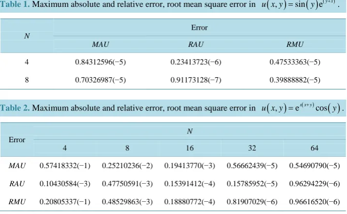
y e(y x+ ). We have computed the solution and pre-sented MAU, RAU and RMU for the developed method for different values of N in Table 1.

Problem 2.

Consider a non linear problem discussed in [2] which, when solving consists of

x y xy

u u

u u

u

= +

in the region

[ ] [ ]

0,1× 0,1 with the boundary conditions _{u x}

( )

, 0 =ex2_,

( )

0, cos

u y = y , for which the ana-lytical solution is found to be u x y

( )

, =ex x y( + )cos

( )

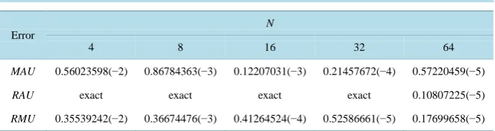
y . We have computed the solution and presented MAU, RAU and RMU for the developed method for different values of N in Table 2.

Problem 3.

Consider a linear problem discussed in [1] which, when solving consists of

3.0

x y xy

u u u

u = + +

in the region

[ ] [ ]

0,1× 0,1 with the boundary conditions

( )

, 0 ex

u x = ,

( )

0, ey

u y = , for which the analytical solution is found to be

( )

, ex y

[image:5.595.120.476.502.721.2]

u x y = + . We have computed the solution and presented MAU, RAU and RMU for the developed method for different values of N in Table 3.

Table 1. Maximum absolute and relative error, root mean square error in u x y

( )

, =sin

( )

y e(y x+).

N

Error

MAU RAU RMU

4 0.84312596(−5) 0.23413723(−6) 0.47533363(−5)

8 0.70326987(−5) 0.91173128(−7) 0.39888882(−5)

Table 2. Maximum absolute and relative error, root mean square error in

( )

, ex x y( )cos

( )

u x y = + y .

Error

N

4 8 16 32 64

MAU 0.57418332(−1) 0.25210236(−2) 0.19413770(−3) 0.56662439(−5) 0.54690790(−5)

RAU 0.10430584(−3) 0.47750591(−3) 0.15391412(−4) 0.15785952(−5) 0.96294229(−6)

(6)

[image:6.595.121.476.99.193.2]

OALibJ | DOI:10.4236/oalib.1100537 6 September 2014 | Volume 1 | e537 Table 3. Maximum absolute and relative error, root mean square error in

(

,

)

ex y

u x y = + .

Error

N

4 8 16 32 64

MAU 0.56023598(−2) 0.86784363(−3) 0.12207031(−3) 0.21457672(−4) 0.57220459(−5)

RAU exact exact exact exact 0.10807225(−5)

RMU 0.35539242(−2) 0.36674476(−3) 0.41264524(−4) 0.52586661(−5) 0.17699658(−5)

5. Conclusions

In general, each numerical method has its own merit and demerit in its application. The present method is there-fore good for use under the initial conditions. The demerit of this method is in computation of initial values which highly affect the all subsequent computational results. The present method which is at least second order accurate seems competitive with other finite difference methods. Method is computationally efficient which can be observed in numerical results obtained in our experiments. It is observed from the results that method has higher accuracy i.e. small discretization error.

In the present article a different approach, we have presented at least second order finite accurate difference method for the numerical solution of the nonlinear Goursat problem. The development of this method will lead to a possibility to further raise the order and accuracy of the method. Work in this direction is in progress and soon it will appear.

References

[1] Day, J.T. (1966) Runge-Kutta Method for the Numerical Solution of the Goursat Problem in Hyperbolic Partial

Diffe-rential Equations. Computer Journal, 9, 81-83. http://dx.doi.org/10.1093/comjnl/9.1.81

[2] Jain, M.K. and Sharma, K.D. (1968) Cubature Method for the Numerical Solution of the Characteristic Initial Value

Problems, u_xy= f x y u u u

(

, , , _x, _y

)

. Journal of the Australian Mathematical Society, 8, 355-368.

http://dx.doi.org/10.1017/S1446788700005425

[3] Evans, D.J. and Sanugi, B.B. (1988) Numerical Solution of the Goursat Problem by a Nonlinear Trapezoidal Formula.

Applied Mathematics Letters, 1, 221-223. http://dx.doi.org/10.1016/0893-9659(88)90080-8

[4] Stetter, H.J. and Torning, W. (1963) General Multistep Finite Difference Method for the Solution of

(

, , , ,

)

xy x y

u = f x y u u u . Rendiconti del Circolo Matematico di Palermo, 12, 281-298.

http://dx.doi.org/10.1007/BF02851264

[5] Nasir, M.A.S. and Ismail, A.I.M. (2005) A New Finite Difference Scheme Based on Heronian Mean Averaging for the

Goursat Problem. ISAME Transactions, 2, 98-103.

[6] Jeffrey, A. and Taniuti T. (1964) Nonlinear Wave Propagation. Academic Press, New York.

[7] Pandey, P.K. (2014) A Fourth Order Finite Difference Method for the Goursat Problem. Acta Technica Jaurinensis, 7,

319-327.

[8] Chawla, M.M. (1979) A Sixth Order Tridiagonal Finite Difference Method for General Nonlinear Two Point Boundary

Value Problems. Journal of the Institute of Mathematics and its Applications, 24, 35-42.