Testing for state dependence in binary panel data with individual covariates

(1)

Munich Personal RePEc Archive

Testing for state dependence in binary

panel data with individual covariates

Bartolucci, Francesco and Nigro, Valentina and Pigini,

Claudia

11 July 2013

Online at

https://mpra.ub.uni-muenchen.de/48233/

(2)

Testing for state dependence in binary panel data with

individual covariates

Francesco Bartolucci

University of Perugia (IT)

bart@stat.unipg.it

Valentina Nigro

Bank of Italy (IT)

valentina.nigro@bancaditalia.it

Claudia Pigini

University of Perugia(IT)

pigini@stat.unipg.it

July 11, 2013

Abstract

We propose a test for state dependence in binary panel data under the dynamic logit model with individual covariates. For this aim, we rely on a quadratic exponential model in which the association between the response variables is accounted for in a different way with respect to more standard formulations. The level of association is measured by a single parameter that may be estimated by a conditional maximum likelihood approach. Under the dynamic logit model, the conditional estimator of this parameter converges to zero when the hypothesis of absence of state dependence is true. This allows us to implement a Wald test for this hypothesis which may be very simply performed and attains the nominal significance level under any struc-ture of the individual covariates. Through an extensive simulation study, we find that our test has good finite sample properties and it is more robust to the presence of (autocorrelated) covariates in the model specification in comparison with other existing testing procedures for state dependence. The test is illustrated by an ap-plication based on data coming from the Panel Study of Income Dynamics.

(3)

1 Introduction

In the analysis of panel data, a question of main interest is if the choice (or the condition)

of an individual in the current period may influence his/her future choice (or condition),

either directly (via the so–called “true state dependence”) or through the presence of

un-observed time-invariant heterogeneity; see Feller (1943) and Heckman (1981). Different

policy consequences may derive from disentangling the individual unobserved

heterogene-ity from the true state dependence, where idiosyncratic shocks may last for a long time.

In the case of binary panel data, a very relevant model in which the effects are

disen-tangled is the dynamic logit model (Hsiao, 2005). This model includes individual-specific

intercepts and, further to time-constant and/or time-varying individual covariates, the

lagged response variable. In particular, the regression coefficient for the lagged response

is a measure of the true state dependence.

A drawback of the dynamic logit model, with respect to the static logit model that

does not include the lagged response among the covariates, is that simple sufficient

statis-tics do not exist for the individual-specific intercepts. Therefore, conditional likelihood

inference becomes more complex and may be performed only under certain conditions

on the distribution of the covariates (Chamberlain, 1993; Honor´e and Kyriazidou, 2000).

We recall that the main advantage of this approach, as other fixed-effects approaches, is

that it does not require to formulate any assumption on the distribution of the individual

intercepts and on the correlation between these effects and the covariates; assumptions of

this type are instead required within the random-effects approach.

In order to test for (true) state dependence, Halliday (2007) developed an interesting

approach which does not require any distributional assumption for the individual-specific

intercepts. However, this approach is explicitly formulated for the case of two time periods

(further to an initial observation) and it cannot be easily applied for panel data with

more than two periods. Moreover, it does not explicitly allow for individual covariates.

(4)

overall sample in strata corresponding to different configurations of these covariates, but

this makes the procedure more complex and its results depending on arbitrary choices.

At least to our knowledge, no other approaches having a complexity comparable to that

of Halliday (2007) exist in the literature for testing for state dependence.

In the econometric literature, Bartolucci and Nigro (2010) introduced a dynamic

model, belonging to the quadratic exponential family (Cox, 1972), which may be used

to analyze binary panel data; its parameters have an interpretation very similar to the

parameters of the dynamic logit model. Moreover, under the model of Bartolucci and

Ni-gro (2010), simple sufficient statistics for the the individual-specific intercepts exist which

are the sums of the response variables at individual level. A conditional maximum

likeli-hood estimator may be then used to estimate the model parameters. Moreover, Bartolucci

and Nigro (2012) showed how to use this technique also for estimating the parameters of

the dynamic logit model. The resulting pseudo conditional maximum likelihood (PCML)

estimator has good performance in comparison with the method proposed by Honor´e and

Kyriazidou (2000) and Carro (2007) and related estimators. In particular, with respect

to the estimator of Honor´e and Kyriazidou (2000), the PCML estimator has the

advan-tage of better exploiting the information in the sample and of allowing for aggregate

time-covariates (such as time-dummies).

In this paper, we propose a test for state dependence based on a modified version

of the quadratic exponential model of Bartolucci and Nigro (2010), which relies on a

different formulation of the structure regarding the conditional association between the

response variables given the individual-specific intercepts for the unobserved heterogeneity

and the covariates. We show that the proposed model may be still represented as a

latent index model where the errors are logistically distributed and the systematic part

is formulated in terms of future expectations. This model may be estimated in a simple

way by a conditional likelihood approach based on the same sufficient statistics as the

(5)

from the dynamic logit model, the estimator of the parameter measuring the association

between the response variables converges to zero in absence of state dependence even in

the presence of covariates. It is then natural to test for state dependence on the basis of

the proposed quadratic exponential model by a Wald test statistic.

The test we propose is directly comparable with the one of Halliday (2007) in terms

of simplicity of implementation. Differently from Halliday’s, our test may be used in

the presence of individual covariates and for panel settings of length greater than two.

In addition, we show that, in the special case of two time periods and no individual

covariates, the two procedures employ the same information in the data to test for state

dependence.

We compared the proposed test with that of Halliday (2007) through a deep simulation

study. It turns out that in absence of individual covariates and with two time occasions,

the two testing approaches perform very similarly in terms of significance level and power,

but in the other cases the former clearly outperforms the latter. In particular, we show

that ignoring the covariates, as Halliday (2007)’s test does, may lead to unsatisfactory

finite–sample properties. Furthermore, the proposed test, which is based on the modified

quadratic exponential model, proves to be more powerful than a Wald test based on more

standard formulations of this model and a test directly based on the PCML estimator.

With the aim of illustrating the proposed test, we consider an application about the

relation between women’s employment and fertility, which is based on a dataset deriving

from the Panel Study of Income Dynamics (PSID). This analysis is related to those

proposed by Hyslop (1999) and Bartolucci and Farcomeni (2009).

The paper is organized as follows. In Section 2 we describe the dynamic logit model

and the alternative quadratic exponential model of Bartolucci and Nigro (2010); for the

purpose of our comparison, in the same section we also illustrate Halliday (2007)’s testing

approach. In Section 3 we introduce the proposed Wald test for state dependence based

(6)

power of this test are studied by simulation in Section 4. Finally, in Section 5 we provide

the empirical illustration based on the PSID dataset. In the last section we draw the

main conclusions.

We make our R _{implementation of all the algorithms illustrated in this paper, and in}

particular of the algorithm to perform the proposed test for state dependence, available

to the reader upon request.

2 Preliminaries

For a panel ofn subjects observed at T time occasions, letyit denote the binary response

variable for subjectiat occasiontand letxitdenote the corresponding vector of individual

covariates. Also let y_i = (yi1, . . . , yiT)′ denote the vector of all outcomes for subjectiand

Xi = (xi1 · · · xiT) denote the matrix of all covariates for this subject.

In the following, we briefly review the dynamic logit model for these data and then

the quadratic exponential model as an alternative model that includes a state dependence

parameter. We also review the test for state dependence proposed by Halliday (2007).

2.1 Dynamic logit model

The dynamic logit model assumes that, for i = 1, . . . , n and t = 1, . . . , T, the binary response yit has conditional distribution

p(yit|αi,Xi, yi0, . . . , yi,t−1) =p(yit|αi,xit, yi,t−1) =

exp[yit(αi+x′itβ+yi,t−1γ)]

1 + exp(αi+x′itβ+yi,t−1γ)

, (1)

where βand γ are the parameters of interest and the individual-specific intercepts αi are

often considered as nuisance parameters; moreover, the initial observation yi0 is given.

Therefore, the joint probability of y_i given αi, Xi, and yi0 has expression

p(y_i|αi,Xi, yi0) = Y

t

p(yit|αi,xit, yi,t−1) =

exp(yi+αi+Ptyitx′itβ+yi∗γ) Q

t[1 + exp(αi+x′itβ+yi,t−1γ)]

(7)

where yi+ =Ptyit and yi∗ =Ptyi,t−1yit, with the product Qt and the sum P

t ranging

over t= 1, . . . , T.

It is important to stress that γ measures the effect of the true state dependence and then the hypothesis on which we focus is H0 : γ = 0, meaning absence of this

form of dependence. The parameter γ may be identified and consistently estimated if the αi parameters are properly taken into account. In particular, Chamberlain (1985)

showed that a conditional approach, in the case of no covariates, may identify the state

dependence parameter by suitable sufficient conditions for the αi parameters. Along

these lines, Honor´e and Kyriazidou (2000) extended the conditional estimator including

exogenous covariates in the model. Under particular conditions on the support of the

covariates, they showed that, for T = 3, y_i is conditionally independent of αi given

the initial and the final observations of the response variable and that yi1 + yi2 = 1.

Their estimator has the advantage, as in any fixed-effects estimator, to let αi be freely

correlated with the covariates in Xi and it does not require to formulate any assumption

on the distribution of these effects. One of its characteristics is that a weight is attached

to each observation; this weight depends on the covariates through a kernel function which

reduces the rate of convergence of the estimator, which is slower than √n. Also due to this condition, the sample size substantially shrinks lowering the overall efficiency of the

estimator. Moreover, this approach does not allow for time-dummies or trend variables

and may be applied only with T > 2, beyond the initial observation.

A different fixed-effects approach is based on bias corrected estimators; see Hahn and

Newey (2004), Carro (2007), Fernandez-Val (2009), and Hahn and Kuersteiner (2011).

They are only consistent as T _{→ ∞} but have a reduced order of bias and they remain asymptotically efficient. For this reason, these estimators are shown to have good

(8)

2.2 Quadratic exponential model

The quadratic exponential model directly defines the joint probability ofy_i given Xi and

yi0, and also given an individual-specific effect here denoted by δi, as follows:

p(y_i|δi,Xi, yi0) =

exp(yi+δi+P_tyitx′itφ+yi∗ψ) P

zexp(z+δi+

P

tztx′itφ+zi∗ψ)

, (2)

where the sum P

z ranges over all the possible binary response vectors z= (z1, . . . , zT)′,

z+ = Ptzt, and zi∗ = yi0z1 +Pt>1zt−1zt. We refer to this model as QE1. Here we

use a different notation from that used for the dynamic logit model, where the vector of

regression coefficients is denoted by φ and the state dependence parameter by ψ. These parameters are collected in the vector θ = (φ′, ψ)′_.

The model is a special case of that proposed by Bartolucci and Nigro (2010) with

the parameters φ assumed to be equal for all time occasions1_{. The same results of their}

paper apply straight to model (2); therefore, the conditional probability of yit may be

represented as

p(yit|δi,Xi, yi0, . . . , yi,t−1) =

exp_{yit[δi+x′itφ+yi,t−1ψ +et(δi,Xi)]}

1 + exp[δi+x′itφ+yi,t−1ψ+et(δi,Xi)]

,

where

et(δi,Xi) = log

1 + exp[δi+x′i,t+1φ+et+1(δi,Xi) +ψ]

1 + exp[δi+x′i,t+1φ+et+1(δi,Xi)]

= logpt+1(yi,t+1 = 0|δi,Xi, yit = 0)

pt+1(yi,t+1 = 0|δi,Xi, yit = 1)

,

for t = 1, . . . , T ₋1, with eT(δi,Xi) = 0. This correction term may be interpreted as

the effect of the current choice yit on the expected utility of the future choice yi,t+1.

Furthermore, the quadratic exponential model shares with the dynamic logit the same

interpretation of the state dependence parameter as log-odds ratio between any pair of

response variables (yi,t−1, yit); moreover, yit is conditionally independent of any other

response variable given yi,t−1 and yi,t+1. Actually, when ψ = 0 this model coincides with

1_{Bartolucci and Nigro (2010) used a different parametrization for}t₌T _{in order to approximate the}

(9)

the static logit model, and this is an important point for the approach here proposed.

The main advantage of model QE1 defined above is the availability of simple

suffi-cient statistics for the unobserved heterogeneity parameters. In particular, the suffisuffi-cient

statistic for each parameter αi is yi+. Therefore, a √n-consistent estimator ˆθ = ( ˆφ ′

,ψˆ)′

may be derived maximizing a likelihood based on the conditional probability

p(y_i|Xi, yi0, yi+) =

exp (P

tyitx′itφ+yi∗ψ)

P

z:z+=yi+exp (

P

tztx′itφ+zi∗ψ)

, (3)

where the sum P

z_:z+=yi+ is extended to all response configurations z with sum equal to

yi+. The estimator may be computed through a Newton-Raphson algorithm. Moreover,

it allows for time-dummies and can be used even with T = 2.

Bartolucci and Nigro (2012) also showed that, up to a correction term, a quadratic

exponential model of the type above may approximate the dynamic logit. On the basis of

this result they derived a PCML estimator which is very competitive in terms of efficiency

compared with the other estimators proposed in the econometric literature. In particular,

this estimator typically results more efficient than the estimator of Honor´e and Kyriazidou

(2000) and it does not impose any conditions on the support of the covariates.

2.3 Available test for state dependence

Halliday (2007) proposed a test for state dependence allowing for the presence of aggregate

time variables in a dynamic logit model of type (1). The proposed approach, which follows

the lines of the conditional approach of Chamberlain (1985), is based on the construction

of conditional probability inequalities that depend only on the sign of the state dependence

parameter γ.

In the case of T = 2, Halliday (2007) considered the events Ai1 = {yi0 = 1, yi1 =

1, yi2 = 0} and Bi1 ={yi0 = 0, yi1 = 1, yi2 = 0} and he proved that

(10)

and

p(Ai1|Xi, yi0 = 1, yi+= 1)≤p(Bi1|Xi, yi0 = 0, yi+ = 1) for γ ≤0,

under assumption (1). Whenxi1 andxi2 are constant across subjects, and therefore there

are only time-dummies common to all sample units, it is possible to consistently estimate

pA=p(Ai1|Xi, yi0 = 1, yi+= 1) and pB =p(Bi1|Xi, yi0 = 0, yi+= 1) as follows

ˆ

pA=

P

i1{Ai1|Xi}

P

i1{yi+ = 1, yi0 = 1|Xi}

= n110

m1

and pˆB =

P

i1{Bi1|Xi}

P

i1{yi+ = 1, yi0 = 0|Xi}

= n010

m0

,

where 1_{·}is the indicator function,ny0y1y2 is the frequency of sample units with response

configuration (y0, y1, y2), andmy0 =ny001+ny010. The test statistic forH0 :γ = 0 is then

defined as

S =√n pˆA−pˆB

ˆ

σ(ˆpA−pˆB)

(4)

where ˆσ(ˆpA−pˆB) is the estimated standard deviation of the numerator. As the sample

size grows to infinity, the test statistic converges to a standard normal distribution only

under H0; otherwise it diverges to +∞ or to −∞, as n grows to infinity, according to

whether γ >0 or γ <0. It is worth noting that the test statistic exploits all the possible configurations of the response variable, conditionally onyi+ = 1; in fact, after some simple

algebra, the numerator of (4) may be written as

ˆ

pA−pˆB =

n001n110−n101n010

m1m0

. (5)

The method of Halliday (2007) identifies the sign of the state dependence parameter

without estimating γ and avoiding distributional assumptions on the unobserved hetero-geneity parameters. Nevertheless, this result cannot be easily generalized for T > 2. A possible solution may be using a multiple testing technique (Hochberg and Tamhane,

1987), where tests for all possible triples (yi,t−1, yit, yi,t+1),t= 1, . . . , T−1, are combined

together. Furthermore, to take into account individual covariates that vary across

(11)

the covariates. Consequently, the results may depend on how the covariate configurations

are taken and may give a final ambiguous solution.

3 Proposed test for state dependence

In the following, we first illustrate a modified version of the quadratic exponential model

QE1 outlined in Section 2.2 and then we show how to test for state dependence on the

basis of the estimates of the parameters of this model.

3.1 Modified quadratic exponential model

To construct a test for state dependence we propose to modify the quadratic exponential

model based on expression (2) in the following way:

˜

p(y_i|δi,Xi, yi0) =

exp(yi+δi+P_tyitx′itφ+ ˜yi∗ψ) P

zexp(zi+δi+

P

tztx′itφ+ ˜zi∗ψ)

, (6)

where ˜yi∗ =Pt1{yit =yi,t−1} and ˜zi∗ = 1{z1 =yi0}+Pt>11{zt =zt−1}, and where we

use ˜p(_·|·) instead of p(_·|·) for the probability function in order to avoid confusion, given that the two models use the same parameters; in particular, the parameters of interest

are still collected in the vector θ. This model is referred to as QE2. The main difference

between models QE1 and QE2 is in how the association between the response variables is

modeled. Here this structure is based on the statistic ˜yi∗ that, differently fromyi∗, is equal

to the number of consecutive pairs of outcomes which are equal each other, regardless if

they are equal to 0 or 1.

Regarding the interpretation of model QE2 based on assumption (6), it useful to

consider how this expression becomes after recursive marginalizations of the response

variables in backward order. In particular, for t = 1, . . . , T ₋1, we have that

˜

p(yi1, . . . , yit|Xi, yi0) =

exp(Pt_h=1yihδi+Pth=1yihx′ihφ+ Pt

h=11{yih=yi,h−1}ψ)˜gt(yit, δi,Xi)

P

zexp(zi+δi+

P

(12)

where

˜

gt(yit, δi,Xi) = ˜gt+1(0, δi,Xi) exp[(1−yit)ψ] + ˜gt+1(1, δi,Xi) exp(δi +x′i,t+1φ+yitψ),

with ˜gT(yiT, δi,Xi) = 1. Consequently, for t = 1, . . . , T, we have that

log p˜(yi1, . . . , yi,t−1, yit = 1|Xi, yi0) ˜

p(yi1, . . . , yi,t−1, yit = 0|Xi, yi0)

=δi+x′itφ+ (2yi,t−1−1)ψ+ ˜et(δi,Xi),

where

˜

et(δi,Xi) = log

˜

gt(1, δi,Xi)

˜

gt(0, δi,Xi)

= log ˜gt+1(0, δi,Xi) + ˜gt+1(1, δi,Xi) exp(δi+x

′

i,t+1φ+ψ)

˜

gt+1(0, δi,Xi) exp(ψ) + ˜gt+1(1, δi,Xi) exp(δi+x′i,t+1φ)

= log 1 + exp[δi +x

′

i,t+1φ+ψ+et+1(δi,Xi)]

exp(ψ) + exp[δi+x′i,t+1φ+ ˜et+1(δi,Xi)]

, (7)

for t= 1, . . . , T ₋1, with ˜eT(δi,Xi) = 0. For t=T, this implies that

˜

p(yit|δi,Xi, yi,t−1) =

exp_{yt[δi +x′itφ+ (2yi,t−1−1)ψ]

1 + exp[δi+x′itφ+ (2yi,t−1−1)ψ]

;

this expression may be seen as a reparametrization of the probability expression holding

under the dynamic logit model (1). For t= 1, . . . , T ₋1, instead, we have

˜

p(yit|δi,Xi, yi,t−1) =

exp_{yt[δi+x′itφ+ (2yi,t−1−1)ψ−ψ+ ˜et(δi,Xi)]

1 + exp[δi+x′itφ+ (2yi,t−1−1)ψ−ψ + ˜et(δi,Xi)]

.

Regarding the interpretation of the last expression, first of all consider that for ψ = 0 definition (7) implies that ˜et(δi,Xi) = 0 and then we have again a reparametrization of

the dynamic logit model. Moreover, it may be easily proved that

˜

et(δi,Xi) = log

˜

p(yi,t+1 = 0|δi,Xi, yit= 0)

˜

p(yi,t+1 = 0|δi,Xi, yit= 1)

.

This correction term depends on the data only through xi,t+1, . . . ,xiT and has a similar

interpretation in terms of the probability of future choices as model QE1 and the quadratic

exponential model of Bartolucci and Nigro (2010).

(13)

dynamic logit model between the response variable yit and yi0, . . . , yi,t−2, yi,t+2, . . . , yiT,

given αi, Xi,yi,t−1, and yi,t+1 (t= 2, . . . , T −1).

Finally, we have

logp˜(yit= 1|δi,Xi, yi,t−1 = 1)

˜

p(yit= 0|δi,Xi, yi,t−1 = 1)

˜

= 2ψ, i= 1, . . . , n, t= 1, . . . , T,

meaning that the log-odds ratio between every consecutive pair of response variables has

the same sign of ψ and it is equal to 0 if there is no state dependence.

3.2 Model estimation and testing for state dependence

As for model QE1, the sums of the response variables at the individual level, yi+, are

sufficient statistics for the individual-specific intercepts δi. Conditioning on the sum of

the response variables, we obtain for model QE2 the following conditional probability

function:

˜

p(y_i|X_i, yi0, yi+) =

exp(P

tyitx′itφ+ ˜yi∗ψ) P

z:z+=yi+exp(

P

, (8)

which directly compares with (3). For making inference on the state dependence

param-eter ψ, the new quadratic exponential model allows us to use a larger set of information with respect to the initial model QE1. This issue will be discussed in more detail at the

end of this session.

On the basis of expression (8), we obtain the conditional log-likelihood

˜

ℓ(θ) =X

i

1_{0< yi+ < T}ℓ˜i(θ), (9)

where

˜

ℓi(θ) = log ˜p(yi|Xi, yi0, yi+)

= X

t

yitx′itφ+ ˜yi∗ψ−log X

z:z+=yi+

exp X

t

ztx′itφ+ ˜zi∗ψ !

(10)

is the individual contribution to the conditional log-likelihood. Note that the response

(14)

Function ˜ℓ(θ) may by maximized by a Newton–Raphson algorithm in a similar way as for model QE1, using the score vector and the information matrix reported below; see

also Bartolucci and Nigro (2010). In this regard, it is convenient to write

˜

ℓi(θ) = ˜u(Xi, yi0,yi)′θ−log X

z_:z+=yi+

exp[˜u(X_i, yi0,z)′θ],

with

˜

u(X_i, yi0,yi) =

X

t

yitx′it,y˜i∗ !′

,

so that, using the standard theory about the regular exponential family, we have the

following expressions for the score for ˜ℓ(θ):

˜

s(θ) = ∇θℓ˜(θ) =

X

i

˜

s_i(θ),

˜

s_i(θ) = ˜u(X_i, yi0,yi)−E˜θ[˜u(X_i, y_i0,y_i)|X_i, y_i0, y_i+].

Regarding the observed information matrix we have

˜

J(θ) =₋∇θθℓ˜(θ) =

X

i

˜

Vθ[˜u(X_i, y_i0,y_i)|X_i, y_i0, y_i+]. (11)

In these expressions, ˜Eθ[˜u(Xi, yi0,yi)|Xi, yi0, yi+] denotes the conditional expected value

of ˜u(Xi, yi0,yi) given Xi and yi+ under model QE2, whereas the corresponding

condi-tional variance is denoted by ˜Vθ[˜u(X_i, y_i0,y_i)|X_i, y_i0, y_i+]. These are given by

˜

Eθ[˜u(Xi, yi0,yi)|Xi, yi0, yi+] =

X

z:z+=yi+

˜

p(z_|Xi, yi0, yi+)˜u(Xi, yi0,z)

˜

Vθ[˜u(X_i, y_i0,y_i)|X_i, y_i0, y_i+] =

X

z:z+=yi+

˜

p(z_|X_i, yi0, yi+)˜d(Xi, yi0,z)˜d(X, yi0,z)′,

with ˜d(Xi, yi0,z) = ˜u(Xi, yi0,z)−E˜θ[˜u(X_i, y_i0,y_i)|X_i, y_i0, y_i+]. Note that ˜J(θ) is

al-ways non-negative definite since it corresponds to the sum of a series of variance-covariance

(15)

The conditional maximum likelihood estimator of θ based on the maximization of (9) is

denoted by ˜θ = ( ˜φ′,ψ˜)′_.

Once the parameters of the proposed quadratic exponential model are estimated, it is

straightforward to construct a standard Wald statistic for testing that ψ = 0, as follows:

W = ψ˜

se( ˜ψ), (12)

where se(_·) is the standard error which is estimated by the sandwich formula reported in

Appendix. It is worth noting that when γ = 0, the dynamic logit model corresponds to the proposed quadratic exponential model QE2 when ψ = 0. This implies the following main result.

Proposition 1 Under the dynamic logit model and if the null hypothesis H0 : γ = 0

holds, the test statistic W defined in (12) has asymptotic standard normal distribution as

n _{→ ∞}.

Moreover, if data are generated from the dynamic logit model but γ ₆= 0, then the value of W is expected to diverge to +_∞ or_−∞ according to whether the true value of

γ is positive or negative. This is because, as we show at the end of Section 3.1, the sign of ψ is the same of the log-odds ratio between pairs of consecutive response variables and the latter is equal to γ under the dynamic logit model. Therefore, within the proposed approach we rejectH0 against the unidirectional alternativeH1 :γ >0 at the significance

level α if the observed value of W is greater than zα, where zα is the 100α-th upper

percentile of the standard normal distribution. Similarly, we rejectH0 against H1 :γ <0

if the observed value of W is smaller than₋zα and we rejectH0 against the bidirectional

alternative H1 :γ 6= 0 if the observed value of |W| is greater than zα/2.

In the following, we illustrate the case with T = 2 and only time dummies con-sidered by Halliday (2007) and illustrated in Section 2.3. In this case, the conditional

log-likelihood of model QE2, as defined in (9), allows us to identify two parameters, that

(16)

for the state dependence, so that θ = (φ, ψ)′_{. Moreover, after some simple algebra we}

have

˜

ℓ(θ) = X

i

1

yi+= 1}{yi2φ+ (1{yi1 =yi0}+ 1{yi2 =yi1})ψ

− log X

z:z+=yi+

exp[z2φ+ (1{z1 =yi0}+ 1{z2 =z1}ψ)

,

that, in terms of sample frequencies, may be expressed as

˜

ℓ(θ) = (n001+n101)φ+ (n001+n110)ψ−m0logk(0)−m1logk(1),

where k(yi0) = exp[φ+ (1−yi0)ψ] + exp(yi0ψ). Consequently, the score function is

˜

s(θ) = X

i

1_{yi+ = 1}

yi2− exp[φ+(1−yi0)ψ]_k(yi0₎

1_{yi1 =yi0} −1{yi1=yi0}exp[(1−y_k(yi0i0)φ+1{y₎ i1=yi0}ψ]

!

= n001+n101−

m0exp(φ+ψ)

k(0) −

m1exp(φ)

k(1)

n001+n110− m0exp(φ+ψ)_k(0) −m1_k(1)exp(ψ)

!

.

In order to solve the system of two equations ˜s(θ) = 0, we initially subtract the first

equation from the second and, after some algebra, we obtain

exp(ψ) = n110

n101

exp(φ). (13)

We then substitute this result in the first equation obtaining

ˆ

φ = 1 2log

n001n101

n010n110

.

Finally, by substituting this solution in (13), we have

ˆ

ψ = 1 2log

n001n110

n010n101

.

This result shows that our test statistic is based on the same response variable

(17)

Moreover, the two test statistics always exhibit the same sign since

sign( ˜ψ) = sign[log(n001n110)−log(n010n101)] = sign(n001n110−n010n101) = sign(ˆpA−pˆB),

where ˆpA−pˆB in the numerator of Halliday’s test statisticS defined in (4). This confirms

that our estimator ˜ψ identifies the sign of the state dependence parameter γ under the dynamic logit model. A consequence is that the proposed test statistic W and the test statistic S have the same asymptotic distribution with mean centered in 0 under the dynamic logit model when H0 : γ = 0 holds; both test statistics diverge to +∞ or −∞ under the dynamic logit model with γ ₆= 0 (the first case when the true value of

γ is positive and the second when it is negative). This is in agreement with the similar performance of the tests based on the two statistics, S andW, in terms of actual size and power that we note in the simulation study (see Section 4) when T = 2 and in absence of individual covariate.

A relevant issue is if the same Wald test as above may be based on the initial quadratic

exponential model QE1, using a statistic of type ˆψ/se( ˆψ), as also this model is equal to the static logit model when ψ = 0. Our conjecture is that this test is less powerful than the test based on the test statisticW defined above, since the latter is based on a version of the quadratic exponential model, the estimator of which better exploits the information

about the association between the response variables. In order to illustrate this point,

we consider the simple case in which there are two time occasions, no covariates, and no

time-dummies. In this case it is possible to prove that the conditional likelihood estimator

of ψ under model QE1 is equal to

ˆ

ψ = logn110

n101

in terms of sample frequencies, whereas, under model QE2, the estimator of this parameter

is equal to

˜

ψ = n001+n110

n010+n101

(18)

Both estimators converge in probability to the true value of γ under the dynamic logit model if H0 : γ = 0 holds. However, the first estimator exploits a reduced amount of

information with respect to the second, as it ignores the response configurations ny0y1y2

with y0 = 0; this also happens in more complex situations. Consequently the test based

on estimator ˆψ (QE1) attains a reduced power than the one based on the estimator ˜ψ

(QE2) when the true value of γ is different from 0. As will be shown in Section 4.2, this different behavior is also confirmed by the simulation results. A related point is how

the proposed test compares with a Wald test based on one of the fixed-effects estimators

for the dynamic logit model, as the PCML estimator proposed by Bartolucci and Nigro

(2012). Since this estimator is based on model QE1, as an approximating model, we

expect a similar difference in terms of power with respect to the proposed test for state

dependence.

4 Simulation study

In order to study the finite–sample properties of the Wald test for state dependence

proposed in Section 3, we performed a comprehensive Monte Carlo experiment based on

a simulation design similar to the one adopted by Honor´e and Kyriazidou (2000).

4.1 Design

In particular, we generated samples from a dynamic logit model where the conditional

mean specification includes individual-specific intercepts, one covariate, and the lag of the

response variable, as follows:

yit = 1{αi+xitβ+yi,t−1γ+εit ≥0},

for i= 1, . . . , n and t = 1, . . . , T, with initial condition

(19)

The error terms εit are independent, and have zero–mean logistic distribution with

vari-ance π2_/_{3. For} _T _≥ _{2, the individual intercepts} _α

i are defined as αi = 1₃P2_t=0xit, where

the covariate xit is generated as

xi0 ∼ N 0, π2/3

,

xit = xi,t−1ρ+uit,

uit ∼ N 0, 1−ρ2

π2/3

,

so that xit and εit have the same stationary variance. In this way, the generating model

admits a correlation between the covariates and the individual-specific intercepts and also

it allows for an autocorrelation of the covariate for the same unit according to an AR(1)

dependence structure. In particular, the covariate is autocorrelated if the parameter ρ is different from 0, whereas if ρis equal to 0 we have a simulation design with independent covariate values at different occasions.

Based on the above generating model, we ran experiments for values of γ on a grid between ₋1.0 and 1.0 with step 0.1. The values of sample size we considered are 500 and 1000; we also considered panels of length T = 2,5,β = 0,1, andρ= 0.5. The number of Monte Carlo replications was fixed at 1,000.

We performed the proposed Wald test for state dependence based on model QE2

comparing its behavior with that of the test of Halliday (2007). An important feature of

the latter is that it does not allow to take into account individual covariates. A possible

solution is performing the test separately for subgroups of individuals (see Section 2.3).

The problem is relevant when the covariates are autocorrelated, as it is reasonable to

expect in standard economic applications. A procedure that ignores the presence of these

explanatory variables may confound state dependence with the persistence that comes

from the correlation of yi,t−1 with xit, as both depend on xit−1. We, therefore, expect

Halliday’s test to exhibit rather wrong size properties in these circumstances.

(20)

dependence when T > 2. In our simulation, we considered all the possible triples

(yi,t−1, yit, yi,t+1), t = 1, . . . , T − 1, computed Halliday’s test for each of these triples

and then decided when to reject H0 :γ = 0 by a multiple testing technique (see Hochberg

and Tamhane, 1987). In particular, H0 is rejected if at least one of the p–values that are

obtained from each of the T ₋1 triples of consecutive observations is smaller than the Bonferroni corrected nominal size. Such a correction ensures that the family-wise error

rate is controlled for. For instance, if we test the null hypothesis for a nominal size of

0.05, the corrected nominal size is 1₋ T

−√1 0.95 for each single test.

4.2 Simulation results

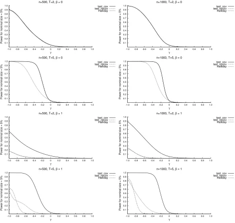
Figure 1 depicts the power curves resulting from the simulation study illustrated in the

previous section for the proposed Wald test based on statistic W defined in (12); and that proposed by Halliday (2007) and based on statistic S defined in (4). For a better comparison with the Halliday’s test (see Section 2.3), we estimated model QE2 on which

our test is based, including the covariatexitand without this covariate. All rejection rates

are displayed for a nominal size α = 0.05 and considering the null hypothesisH0 :γ = 0

against the bidirectional alternative hypothesis H1 : γ 6= 0. For the Wald test statistic,

the curve labelled by “test cov” refers to the situation in which xit is included in the

model specification; the curve is labelled by “test nocov” when this covariate is ignored.

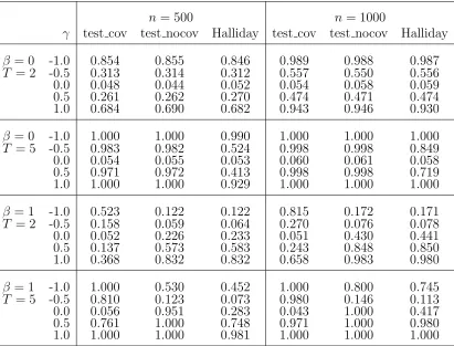
For certain relevant values of γ, Table 1 displays the rejection rate of this bidirectional test.

[Figure 1 about here.]

[Table 1 about here.]

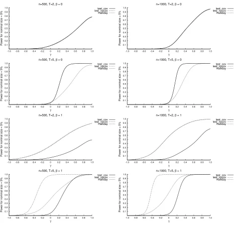
For each approach, we also considered both lower and upper tailed tests (Figures 2 and

(21)

[Figure 3 about here.]

The top panels of Figures 1–3 show that the proposed test has size equal to the

nominal level α when β = 0 and T = 2 and with both sample sizes, whereas a sample size of at least 1000 is needed to exhibit satisfactory power properties. In these scenarios,

Halliday’s test statistic presents a behavior very similar to the proposed test. WithT = 5 and β = 0, the rejection rate for the proposed test sensibly increases (see the second–row panels of Figures 1–3) reaching almost 100% for _|γ_| = 0.6 (with n = 500) and _|γ_| = 0.4 (with n = 1000). On the contrary, the generalization of Halliday’s test statistic to cases with T > 2 leads to a remarkable power loss: with n = 500 and _|γ_| = 0.5 the rejection rate is about one half of that of the proposed test (see Table 1).

The third and fourth row–panels of Figures 1–3 provide an illustration of the simulation

results withβ= 1. While the proposed “test cov” maintains its size properties, Halliday’s test over-rejects the null hypothesis of absence of state dependence when this hypothesis

is true. Moreover, the test size bias grows with the sample size: when T = 2, for example, it rises from 23% withn = 500 to 44% withn= 1000 (see Table 1). As expected, ignoring the presence of the covariate xitin testing for state dependence leads to mistakenly detect

a significant persistence in the dependent variable. This result is also confirmed by the

rejection rates of “test nocov” that exhibit the same behavior as Halliday’s. Regarding

the power, it decreases for all the three tests when β = 1 rather thanβ = 0. Nevertheless, our test shows a better performance in the case γ <0. On the other hand, forγ >0 and

T = 2 this test has less power than Halliday’s, which, however, confounds the positive autocorrelation in the covariate with a positive state dependence.

In conclusion, the above simulation results confirm our conjecture that in absence

of individual covariates and when T = 2, the proposed Wald test for state dependence performs similarly, in terms of size and power, to the test proposed by Halliday (2007).

Furthermore, in all other situations, our test is superior to the other one, mainly due to

(22)

individual covariates.

A final point concerns performing a Wald test for state dependence which is based

on the initial quadratic exponential model QE1 defined in (2). We recall that the main

difference with the model here adopted for the test (QE2) is in the way the association

between the response variables is accounted for. In this regard, Table 2 shows the Monte

Carlo results for the test based on model QE1 and in particular on the estimator of ψ

coming from the maximization of conditional likelihood (3).

As expected, the power properties of the test based on the initial QE1 model are less

satisfactory compared to those of the proposed test. This is due to an information loss:

model QE1 only considers the information concerning pairs of consecutive observations

such that (yi,t−1 = 1, yit = 1). Nevertheless, this test shows a better size with respect to

Halliday’s, in particular for β = 1.

5 Empirical application

In this section, we illustrate an application of the proposed testing procedure based on

a dataset derived from the Panel Study of Income Dynamics2_{. Our example closely}

resembles the empirical analyses in Hyslop (1999) and in Bartolucci and Farcomeni (2009)

that focus on the effect of fertility on women’s employment and on the magnitude of the

state dependence effect in both variables.

For the purposes of the present article, we restrict the analysis to testing for state

dependence for women’s employment and fertility. The dataset concernsn= 1446 married women between 18 and 46 years of age followed for T = 5 time occasions, from 1987 to 1992 (the first year of observation is taken as initial condition). The covariates in the

model specification are: number of children in the family between 1 and 2 years of age

(23)

“child 1-2” and, similarly, “child 3-5”, “child 6-14”, “child 14-”, “income” of the husband

in dollars, time-dummies, “lagged employment”, and “lagged fertility”.

We computed the proposed Wald test statistic for H0 : γ = 0, which is based on the

modified the quadratic exponential model QE2 defined in (8), and the Halliday’s test

statistic defined in (4) for each triple (yi,t−1, yit, yi,t+1), t = 1, . . . , T −1, applying the

Bonferroni corrected nominal size (see Section 4).

In the case the null hypothesis of no state dependence is rejected, it is necessary to

estimate the model parameters in a dynamic framework. As illustrated in Section 2.2,

suitable approaches are based on the conditional estimator of Honor´e and Kyriazidou

(2000), the PCML estimator (Bartolucci and Nigro, 2012), or biased-corrected

fixed-effects estimators (Carro, 2007). If the null hypothesis is not rejected, we simply estimate

a static logit model.

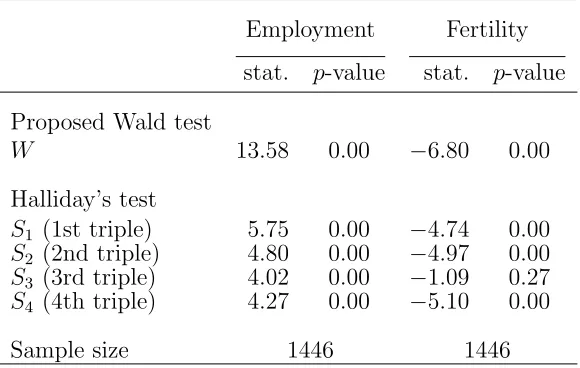
For the dataset here considered, Table 3 reports the test statistics computed by the

different approaches using the complete sample of n = 1446 women. The proposed test strongly rejects the null hypothesis of absence of state dependence for both response

variables employment and fertility. The signs of Halliday’s test statistics also indicate

positive state dependence for employment and negative for fertility. The values of these

statistics are such that the null hypothesis is rejected: in both cases there is at least one

p–value lower than the Bonferroni corrected nominal size.

Since the null hypothesis of absence of state dependence is rejected, we estimated the

dynamic logit model by the PCML estimator. The estimation results, reported in Table 4,

confirm a strong positive state dependence for employment with an estimated coefficient

ˆ

γ close to 1.5 and a negative state dependence for fertility with ˆγ equal to₋0.9. However, in the second case, the value of the Wald test statistic based on this estimate is closer to

zero than the value of the proposed Wald test statistic. The difference is that the PCML

(24)

and then it leads to a less powerful test with respect to the proposed approach based on

model QE2.

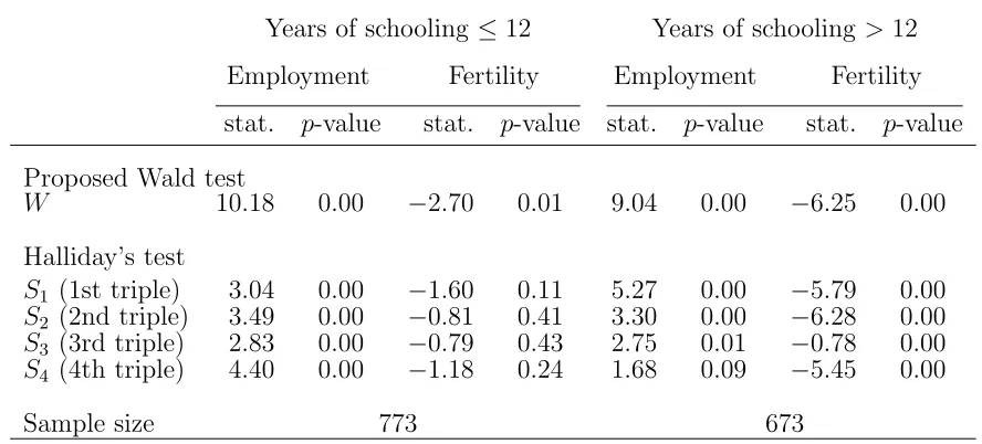
As discussed in Section 2.3, in order for Halliday’s procedure to take into account

observed heterogeneity in terms of individual covariates, the test must be performed

sep-arately for different configurations of such covariates. As an illustration, we performed

this test for two different groups of women created on the basis of the covariate

“educa-tion”: we grouped observations of women with at most 12 years of schooling and those of

women with more than 12 years of schooling (12 is the education median value). Table 5

shows the test statistics for the two groups: in both cases the positive state dependence

in employment is detected by all the test statistics, as they reject H0.

On the contrary, Halliday’s test does not seem to detect the negative state dependence

in fertility for less educated women; this is an important difference with respect to our

approach. For this subsample, the PCML estimate of the state dependence parameter

is negative (equal to ₋0.14; see Table 6) but not significantly different form 0. Overall, in this case the higher power of the proposed testing approach emerges over both the

Halliday’s approach and the approach based on the PCML estimator.

Finally, for women with more than 12 years of schooling, there is agreement between

all the tests which reject the null hypothesis of absence of state dependence in fertility.

For this subsample, the PCML estimate of γ is equal to₋1.3 (see Table 7).

(25)

6 Conclusions

In this paper, we propose a test for state dependence under the dynamic logit model with

individual covariates. The test is based on a modified version of the quadratic exponential

model proposed in Bartolucci and Nigro (2010) in order to exploit more information

about the association between the response variables. We show that this model correctly

identifies the presence of state dependence regardless of whether individual covariates are

present or not.

Our test directly compares with the one proposed by Halliday (2007), which, however,

cannot be easily applied in a panel with more than two periods (further to the initial

observation) and does not allow for individual covariates. In the special case of two time

periods and no covariates, the proposed test employs the same information on the response

variables as Halliday’s.

We studied the finite–sample properties of the Wald test for state dependence proposed

in this paper by means of a comprehensive Monte Carlo experiment in which we also

compare it with the test proposed by Halliday (2007). Simulation results show that the

proposed test attains the nominal size even with not large samples (500 sample units),

while it exhibits satisfactory power properties with large sample sizes. As expected,

ignoring the presence of time-varying covariates in testing for state dependence leads to

mistakenly detect a significant persistence in the response variable: the proposed test

maintains its size properties, whereas Halliday’s test over-rejects the true null hypothesis

of absence of state dependence. Moreover, when state dependence is negative and the

covariate positively affects the response variable, Halliday’s test shows a remarkable power

loss.

This result is confirmed by our empirical study based on a dataset derived from the

Panel Study of Income Dynamics: when using either the whole sample or different

subsam-ples, the proposed test always rejects the null hypothesis of absence of state dependence

(26)

the state dependence.

Overall, the main advantages of the proposed test are the simplicity of use and its

flexibility. In fact, it can be very simply performed and does not require to formulate

any parametric assumption on the distribution of the individual-specific intercepts (or on

the correlation between these intercepts and the covariates) as random-effects approaches

instead require. Moreover, it may be used even with only two time occasions (further

to an initial observations) and with individual covariates of any nature (time-constant or

time-varying), including time-dummies. It is also worth noting that, as in typical

fixed-effects approaches, how the time-constant covariates affect the response variables needs

not to be specified, as their effect is absorbed into to the individual-specific intercepts.

Finally, it is worth noting that the proposed test, being based on a modified quadratic

exponential model, is more powerful than a Wald test based on more traditional quadratic

exponential models or on the pseudo conditional likelihood estimator of Bartolucci and

Nigro (2012). We noticed this aspect in the simulation study and in the empirical

appli-cation.

Acknowledgments

Francesco Bartolucci and Claudia Pigini acknowledge the financial support from the grant

RBFR12SHVV of the Italian Government (FIRB project “Mixture and latent variable

models for causal inference and analysis of socio-economic data”).

Appendix: the standard error of conditional maximum

likelihood estimator

In order to derive an expression for the standard error used in the Wald test statistic, we

(27)

in (10), the variance covariance matrix of ˜θ is

˜

V(˜θ) = ˜J(˜θ)−1H˜(˜θ)[ ˜J(˜θ)−1]′,

where

˜

H(θ) =X

i

1_{0< yi+ < T}s˜i(θ) ˜si(θ)′

and ˜J(θ) is the information matrix defined in (11). Once the matrix ˜V(˜θ) has been

computed as above, the standard error for ˜ψ may be obtained in the usual way from the main diagonal of this matrix.

References

Bartolucci, F. and Farcomeni, A. (2009). A multivariate extension of the dynamic logit

model for longitudinal data based on a latent markov heterogeneity structure. Journal

of the American Statistical Association, 104(486):816–831.

Bartolucci, F. and Nigro, V. (2010). A dynamic model for binary panel data with

unob-served heterogeneity admitting a √n-consistent conditional estimator. Econometrica, 78:719–733.

Bartolucci, F. and Nigro, V. (2012). Pseudo conditional maximum likelihood estimation of

the dynamic logit model for binary panel data. Journal of Econometrics, 170:102–116.

Carro, J. (2007). Estimating dynamic panel data discrete choice models with fixed effects.

Journal of Econometrics, 140:503–528.

Chamberlain, G. (1985). Heterogeneity, omitted variable bias, and duration dependence.

In Heckman, J. J. and Singer, B., editors, Longitudinal analysis of labor market data.

Cambridge University Press: Cambridge.

Chamberlain, G. (1993). Feedback in panel data models. Technical report, Department

(28)

Cox, D. (1972). The analysis of multivariate binary data. Applied statistics, 21:113–120.

Feller, W. (1943). On a general class of ”contagious” distributions.Annals of Mathematical

Statistics, 14:389–400.

Fernandez-Val, I. (2009). Fixed effects estimation of structural parameters and marginal

effects in panel probit model. Journal of Econometrics, 150:71–85.

Hahn, J. and Kuersteiner, G. (2011). Bias reduction for dynamic nonlinear panel models

with fixed effects. Econometric Theory, 27:1152–1191.

Hahn, J. and Newey, W. (2004). Jackknife and analytical bias reduction for nonlinear

panel models. Econometrica, 72:1295–1319.

Halliday, T. H. (2007). Testing for state dependence with time-variant transition

proba-bilities. Econometric Reviews, 26:685–703.

Heckman, J. (1981). Heterogeneity and state dependence. In Rosen, S., editor, Studies

in labor markets, pages 91–140. Chicago University Press: Chicago.

Hochberg, Y. and Tamhane, A. (1987). Multiple comparison procedures. Wiley series in

probability and mathematical statistics: Applied probability and statistics. Wiley.

Honor´e, B. E. and Kyriazidou, E. (2000). Panel data discrete choice models with lagged

dependent variables. Econometrica, 68:839–874.

Hsiao, C. (2005). Analysis of Panel Data. Cambridge University Press, New York, 2nd

edition.

Hyslop, D. R. (1999). State dependence, serial correlation and heterogeneity in

intertem-poral labor force participation of married women. Econometrica, 67(6):1255–1294.

(29)

[image:29.612.86.557.107.552.2]

Figure 1: Power plots for Wald (QE2) and Halliday’s tests: bidirectional (H1 :γ 6= 0) 0.1 0.2 0.3 0.4 0.5 0.6 0.7 0.8 0.9 1.0

-1.0 -0.8 -0.6 -0.4 -0.2 0 0.2 0.4 0.6 0.8 1.0

Power for nominal size = 5%

γ n=500, T=2, β = 0

test_cov test_nocov Halliday 0.1 0.2 0.3 0.4 0.5 0.6 0.7 0.8 0.9 1.0

-1.0 -0.8 -0.6 -0.4 -0.2 0 0.2 0.4 0.6 0.8 1.0

γ

n=1000, T=2, β = 0

-1.0 -0.8 -0.6 -0.4 -0.2 0 0.2 0.4 0.6 0.8 1.0

γ n=500, T=5, β = 0

-1.0 -0.8 -0.6 -0.4 -0.2 0 0.2 0.4 0.6 0.8 1.0

γ n=1000, T=5, β = 0

-1.0 -0.8 -0.6 -0.4 -0.2 0 0.2 0.4 0.6 0.8 1.0

γ n=500, T=2, β = 1

-1.0 -0.8 -0.6 -0.4 -0.2 0 0.2 0.4 0.6 0.8 1.0

γ n=1000, T=2, β = 1

-1.0 -0.8 -0.6 -0.4 -0.2 0 0.2 0.4 0.6 0.8 1.0

γ n=500, T=5, β = 1

-1.0 -0.8 -0.6 -0.4 -0.2 0 0.2 0.4 0.6 0.8 1.0

γ n=1000, T=5, β = 1

test_cov test_nocov Halliday

(“test cov” refers to the case in which the covariate xit is included in the QE2 model; “test nocov” is

(30)

[image:30.612.87.558.170.617.2]

Figure 2: Power plots for Wald (QE2) and Halliday’s tests: lower tailed (H1 :γ <0) 0.1 0.2 0.3 0.4 0.5 0.6 0.7 0.8 0.9 1.0

-1.0 -0.8 -0.6 -0.4 -0.2 0 0.2 0.4 0.6 0.8 1.0

γ n=500, T=2, β = 0

-1.0 -0.8 -0.6 -0.4 -0.2 0 0.2 0.4 0.6 0.8 1.0

γ n=1000, T=2, β = 0

-1.0 -0.8 -0.6 -0.4 -0.2 0 0.2 0.4 0.6 0.8 1.0

γ n=500, T=5, β = 0

-1.0 -0.8 -0.6 -0.4 -0.2 0 0.2 0.4 0.6 0.8 1.0

γ n=1000, T=5, β = 0

-1.0 -0.8 -0.6 -0.4 -0.2 0 0.2 0.4 0.6 0.8 1.0

γ n=500, T=2, β = 1

-1.0 -0.8 -0.6 -0.4 -0.2 0 0.2 0.4 0.6 0.8 1.0

γ n=1000, T=2, β = 1

-1.0 -0.8 -0.6 -0.4 -0.2 0 0.2 0.4 0.6 0.8 1.0

γ

n=500, T=5, β = 1

-1.0 -0.8 -0.6 -0.4 -0.2 0 0.2 0.4 0.6 0.8 1.0

γ

n=1000, T=5, β = 1

(31)

[image:31.612.87.557.162.614.2]

Figure 3: Power plots for Wald (QE2) and Halliday’s tests: upper tailed (H1 :γ >0) 0.1 0.2 0.3 0.4 0.5 0.6 0.7 0.8 0.9 1.0

-1.0 -0.8 -0.6 -0.4 -0.2 0 0.2 0.4 0.6 0.8 1.0

γ n=500, T=2, β = 0

-1.0 -0.8 -0.6 -0.4 -0.2 0 0.2 0.4 0.6 0.8 1.0

γ n=1000, T=2, β = 0

-1.0 -0.8 -0.6 -0.4 -0.2 0 0.2 0.4 0.6 0.8 1.0

γ n=500, T=5, β = 0

-1.0 -0.8 -0.6 -0.4 -0.2 0 0.2 0.4 0.6 0.8 1.0

γ n=1000, T=5, β = 0

-1.0 -0.8 -0.6 -0.4 -0.2 0 0.2 0.4 0.6 0.8 1.0

γ n=500, T=2, β = 1

-1.0 -0.8 -0.6 -0.4 -0.2 0 0.2 0.4 0.6 0.8 1.0

γ n=1000, T=2, β = 1

-1.0 -0.8 -0.6 -0.4 -0.2 0 0.2 0.4 0.6 0.8 1.0

γ n=500, T=5, β = 1

-1.0 -0.8 -0.6 -0.4 -0.2 0 0.2 0.4 0.6 0.8 1.0

γ n=1000, T=5, β = 1

(32)

[image:32.612.109.520.96.409.2]

Table 1: Simulation results for Wald (QE2) and Halliday’s test statistics: bidirectional

n = 500 n= 1000

γ test cov test nocov Halliday test cov test nocov Halliday

β = 0 -1.0 0.854 0.855 0.846 0.989 0.988 0.987

T = 2 -0.5 0.313 0.314 0.312 0.557 0.550 0.556

0.0 0.048 0.044 0.052 0.054 0.058 0.059

0.5 0.261 0.262 0.270 0.474 0.471 0.474

1.0 0.684 0.690 0.682 0.943 0.946 0.930

β = 0 -1.0 1.000 1.000 0.990 1.000 1.000 1.000

T = 5 -0.5 0.983 0.982 0.524 0.998 0.998 0.849

0.0 0.054 0.055 0.053 0.060 0.061 0.058

0.5 0.971 0.972 0.413 0.998 0.998 0.719

1.0 1.000 1.000 0.929 1.000 1.000 1.000

β = 1 -1.0 0.523 0.122 0.122 0.815 0.172 0.171

T = 2 -0.5 0.158 0.059 0.064 0.270 0.076 0.078

0.0 0.052 0.226 0.233 0.051 0.430 0.441

0.5 0.137 0.573 0.583 0.243 0.848 0.850

1.0 0.368 0.832 0.832 0.658 0.983 0.980

β = 1 -1.0 1.000 0.530 0.452 1.000 0.800 0.745

T = 5 -0.5 0.810 0.123 0.073 0.980 0.146 0.113

0.0 0.056 0.951 0.283 0.043 1.000 0.417

0.5 0.761 1.000 0.748 0.971 1.000 0.980

1.0 1.000 1.000 0.981 1.000 1.000 1.000

(33)

[image:33.612.162.466.132.310.2]

Table 2: Simulation results for Wald test (QE1) test statistic: bidirectional

n = 500 n= 1000

γ test cov test nocov test cov test nocov

β = 0 -1.0 0.709 0.710 0.935 0.933

T = 2 -0.5 0.195 0.191 0.351 0.354

0.0 0.045 0.050 0.050 0.056

0.5 0.130 0.130 0.220 0.222

1.0 0.268 0.268 0.483 0.480

β = 1 -1.0 0.347 0.102 0.600 0.149

T = 2 -0.5 0.110 0.058 0.169 0.062

0.0 0.039 0.148 0.045 0.246

0.5 0.091 0.311 0.136 0.525

1.0 0.158 0.448 0.308 0.772

referred to the case in which the covariate is not included)

Table 3: Tests for state dependence (H1 : γ 6= 0): proposed Wald test (QE2) and

Halli-day’s test statistics for the overall PSID dataset

Employment Fertility

stat. p-value stat. p-value Proposed Wald test

W 13.58 0.00 ₋6.80 0.00 Halliday’s test

S1 (1st triple) 5.75 0.00 −4.74 0.00

S2 (2nd triple) 4.80 0.00 −4.97 0.00

S3 (3rd triple) 4.02 0.00 −1.09 0.27

S4 (4th triple) 4.27 0.00 −5.10 0.00

Sample size 1446 1446

[image:33.612.169.459.483.667.2]

(34)

[image:34.612.91.562.152.337.2]

Table 4: Estimation results based on the PCML approach (Bartolucci and Nigro, 2012): overall PSID dataset

coeff. s.e. Wald-stat. p-value coeff. s.e. Wald-stat. p-value

Child 1–2 -0.675 0.13 -5.10 0.00 -0.719 0.15 -4.72 0.00

Child 3–5 -0.312 0.12 -2.52 0.01 -1.085 0.21 -5.05 0.00

Child 6–13 -0.032 0.12 -0.25 0.40 -1.055 0.26 -4.08 0.00

Child 14– -0.010 0.14 -0.07 0.47 -0.800 0.43 -1.86 0.03

Income/1000 -0.007 0.00 -1.68 0.05 -0.000 0.00 -0.13 0.45

1989 0.089 0.14 -1.12 0.13 0.402 0.15 4.64 0.00

1990 0.317 0.13 0.65 0.26 0.445 0.19 2.64 0.00

1991 0.089 0.13 2.49 0.01 0.397 0.24 2.31 0.01

1992 0.001 0.13 0.67 0.25 0.448 0.29 1.66 0.05

Lag fertility -0.185 0.17 0.01 0.50 -0.906 0.21 1.56 0.06

Lag employment 1.550 0.11 13.93 0.00 0.801 0.17 -4.35 0.00

Table 5: Tests for state dependence (H1 : γ 6= 0): proposed Wald test (QE2) and

Halli-day’s test statistics for the PSID dataset

Years of schooling _≤12 Years of schooling >12

Employment Fertility Employment Fertility

stat. p-value stat. p-value stat. p-value stat. p-value Proposed Wald test

W 10.18 0.00 ₋2.70 0.01 9.04 0.00 ₋6.25 0.00 Halliday’s test

S1 (1st triple) 3.04 0.00 −1.60 0.11 5.27 0.00 −5.79 0.00

S2 (2nd triple) 3.49 0.00 −0.81 0.41 3.30 0.00 −6.28 0.00

S3 (3rd triple) 2.83 0.00 −0.79 0.43 2.75 0.01 −0.78 0.00

S4 (4th triple) 4.40 0.00 −1.18 0.24 1.68 0.09 −5.45 0.00

Sample size 773 673

[image:34.612.90.534.473.674.2]

(35)

[image:35.612.91.561.156.341.2]

Table 6: Estimation results based on the PCML approach (Bartolucci and Nigro, 2012): PSID dataset for the subsample with years of schooling _≤12

Child 1–2 -0.419 0.20 -2.12 0.02 -0.726 0.24 -2.96 0.00

Child 3–5 0.055 0.17 0.32 0.33 -0.750 0.33 -2.26 0.02

Child 6–13 0.127 0.16 0.77 0.22 -0.524 0.38 -1.36 0.17

Child 14– 0.067 0.17 0.38 0.35 -0.757 0.69 -1.10 0.27

Income/1000 -0.018 0.01 -2.47 0.01 -0.004 0.01 -0.27 0.78

1989 0.153 0.19 0.13 0.45 0.328 0.23 3.99 0.00

1990 0.193 0.17 0.82 0.20 0.189 0.29 1.41 0.16

1991 0.341 0.18 1.13 0.13 0.004 0.36 0.66 0.51

1992 -0.102 0.18 1.92 0.03 -0.516 0.46 0.01 0.99

Lag fertility 0.031 0.25 -0.57 0.28 -0.145 0.32 -1.13 0.26

Lag employment 1.529 0.15 10.10 0.00 1.090 0.27 -0.45 0.65

Table 7: Estimation results based on the PCML approach (Bartolucci and Nigro, 2012): PSID dataset for the subsample with years of schooling >12

Child 1–2 -0.932 0.19 -0.86 0.19 -0.763 0.20 -3.89 0.00

Child 3–5 -0.690 0.19 -0.64 0.19 -1.350 0.29 -4.68 0.00

Child 6–13 -0.220 0.21 -4.95 0.00 -1.438 0.36 -3.99 0.00

Child 14– -0.154 0.25 -3.59 0.00 -0.811 0.61 -1.34 0.09

Income/1000 -0.001 0.00 -1.05 0.15 -0.000 0.00 -0.02 0.49

1989 0.038 0.29 -0.61 0.27 0.529 0.21 2.99 0.00

1990 0.505 0.20 -0.24 0.41 0.670 0.26 2.57 0.01

1991 -0.139 0.21 -1.43 0.08 0.694 0.33 2.53 0.01

1992 0.208 0.21 0.18 0.43 1.071 0.39 2.10 0.02

Lag fertility -0.325 0.23 2.57 0.01 -1.275 0.28 2.71 0.00

[image:35.612.92.560.495.679.2]