Distributed Memory Parallel Algorithms for
Minimum Spanning Trees
Vladmir Lonˇcar, Srdjan ˇSkrbi´c and Antun Balaˇz
Abstract—Finding a minimum spanning tree of a graph is
a well known problem in graph theory with many practical applications. We study serial variants of Prim’s and Kruskal’s algorithm and present their parallelization targeting message passing parallel machine with distributed memory. We consider large graphs that can not fit into memory of one process. Experimental results show that Prim’s algorithm is a good choice for dense graphs while Kruskal’s algorithm is better for sparse ones. Poor scalability of Prim’s algorithm comes from its high communication cost while Kruskal’s algorithm showed much better scaling to larger number of processes.
Index Terms—Minimum spanning tree, parallel algorithms,
message passing, distributed memory computer.
I. INTRODUCTION
A
MINIMUM spanning tree (MST) of a weighted graph G= (V, E)is a subset ofEthat forms a spanning tree of Gwith minimum total weight. MST problem has many applications in computer and communication network design, as well as indirect applications in fields such as computer vision and cluster analysis [1].In this paper we implement two parallel algorithms for finding MST of a graph, based on classical algorithms of Prim [2] and Kruskal [3]. Algorithms target message passing parallel machine with distributed memory. Primary characteristic of this architecture is that the cost of inter-process communication is high in comparison to cost of computation. Our goal was to develop algorithms which minimize communication, and to measure the impact of com-munication on the performance of algorithms. Our primary interest were graphs which have significantly larger number of vertices than processors involved in computation. Since graphs of this size cannot fit into the memory of a single process, we use a partitioning scheme to divide the input graph among processes. We consider both sparse and dense graphs.
First algorithm is a parallelization of Prim’s serial algo-rithm. Each process is assigned a subset of vertices and in each step of computation, every process finds a candidate minimum-weight edge connecting one of its vertices to MST.
Manuscript received March 7, 2013; revised March 30, 2013. Authors are partially supported by Ministry of Education and Science of the Republic of Serbia, through projects no. ON174023: “Intelligent techniques and their integration into wide-spectrum decision support”, and ON171017: “Modeling and numerical simulations of complex many-body systems”, as well as European Commission through FP7 projects PRACE-2IP and PRACE-3IP.
V. Lonˇcar is with the Department of Mathematics and Informat-ics, Faculty of Science, University of Novi Sad, Serbia, e-mail: [email protected].
S. ˇSkrbi´c (corresponding author) is with the Department of Mathematics and Informatics, Faculty of Science, University of Novi Sad, Serbia, e-mail: [email protected].
A. Balaˇz is with the Institue of Physics, University of Belgrade, Serbia, e-mail: [email protected]
The root process collects those candidates and selects one with minimum weight which it adds to MST and broadcasts result to other processes. This step is repeated until every vertex is in MST.
Second algorithm is based on Kruskal’s approach. Pro-cesses get a subset ofGin the same way as in first algorithm, and then find local minimum spanning tree (or forest). Next, processes merge their MST edges until only one process remains, which holds edges that form MST ofG.
Implementations of these algorithms are done using C programming language and MPI (Message Passing Interface) and tested on a parallel cluster PARADOX using up to 256 cores and 256 GB of distributed memory.
Next section contains references to the most important related papers. In section III we continue with the description and analysis of algorithms - both serial and parallel versions, and their implementation. In the last section we describe experimental results, analyze them and draw our conclusions.
II. RELATEDWORK
A
LGORITHMS for MST problem have mostly been based on one of three approaches, that of Boruvka [4], Prim [2] and Kruskal [3], however, a number of new algorithms has been developed. Gallager et al. presented an algorithm where processor exists at each node of the graph (thusn=p), useful in computer network design [5]. Katriel and Sanders designed an algorithm exploiting cycle property of a graph targeting dense graph, [6], while Ahrabian and Nowzari-Dalini’s algorithm relies on depth first search of the graph [7].Due to its parallel nature, Boruvka’s algorithm (also known as Sollin’s algorithm) has been the subject to most research related to parallel MST algorithms. Examples of algorithms based on Boruvka’s approach include Chung and Condon [8], Wang and Gu [9] and Dehne and G¨otz [10].
Parallelization of Prim’s algorithm has been presented by Deo and Yoo [11]. Their algorithm targets shared memory computers. Improved version of Prim’s algorithm has been presented by Gonina and Kale [12]. Their algorithm adds multiple vertices per iteration, thus achieving significant speedups. Another approach targeting shared memory com-puters presented by Setia et al. [13] uses the cut property of a graph to grow multiple trees in parallel. Hybrid approach, combining both Boruvka’s and Prim’s approaches has been developed by Bader and Cong [14].
Bulk of the research into parallel MST algorithms has tar-geted shared memory computers like PRAM, i.e. computers where entire graph can fit into memory. Our algorithms target distributed memory computers and use partitioning scheme to divide the input graph evenly among processors. Because no process contains info about partition of other processes, we designed our algorithms to use predictable communication patterns, and not depend on the properties of input graph.
III. THEALGORITHMS
L
ET us assume that graph G = (V, E), with vertex set V and edge set E is connected and undirected. Without loss of generality, it can be assumed that each weight is distinct, thus G is guaranteed to have only one MST. This assumption simplifies implementation, otherwise a numbering scheme can be applied to edges with same weight, at the cost of additional implementation complexity. Letn be the number of vertices, mthe number of edges (|V|=n,|E|=m), andpthe number of processes involved in computation of MST. Letw(v, u)denote weight of edge connecting verticesvandu. Input graphGis represented as n×n adjacency matrixA= (ai,j)defined as:ai,j=
(
w(vi, vj) if(vi, vj)∈E
0 otherwise (1)
A. Prim’s Algorithm
Prim’s algorithm starts from an arbitrary vertex and then grows the MST by choosing a new vertex and adding it to MST in each iteration. Vertex with an edge with lightest weight incident on the vertices already in MST is added in every iteration. The algorithm continues until all the vertices have been added to the MST. This algorithm requiresO(n2)
time. Implementations of Prim’s algorithm commonly use auxiliary arraydof lengthnto store distances (weight) from each vertex to MST. In every iteration a lightest weight edge indis added to MST anddis updated to reflect changes.
Parallelizing the main loop of Prim’s algorithm is difficult [17], since after adding a vertex to MST lightest edges incident on MST change. Only two steps can be parallelized: selection of the minimum-weight edge connecting a vertex not in MST to a vertex in MST, and updating arraydafter a vertex is added to MST. Thus, parallelization can be achieved in the following way:
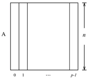
1) Partition the input set V into p subsets, such that each subset containsn/pconsecutive vertices and their edges, and assign each process a different subset. Each process also contains part of arraydfor vertices in its partition. LetVi be the subset assigned to process pi,
anddipart of arraydwhichpi maintains. Partitioning
of adjacency matrix is illustrated in Fig. 1.
2) Every processpi finds minimum-weight edgeei
(can-didate) connecting MST with a vertex inVi.
3) Every processpi sends itsei edge to the root process
using all-to-one reduction.
4) From the received edges, the root process selects one with a minimum weight (called global minimum-weight edgeemin), adds it to MST and broadcasts it
[image:2.595.353.497.54.187.2]to all other processes.
Fig. 1. Partitioning of adjacency matrix amongpprocesses
5) Processes mark vertices connected byemin as
belong-ing to MST and update their part of arrayd. 6) Repeat steps 2-5 until every vertex is in MST.
Finding a minimum-weight edge and updating ofdiduring
each iteration costsO(n/p). Each step also adds a communi-cation cost of all-to-one reduction and all-to-one broadcast. These operations complete in O(logp). Combined, cost of one iteration isO(n/p+ logp). Since there areniterations, total parallel time this algorithm runs in is:
Tp=O
n2
p
+O(nlogp) (2)
Prim’s algorithm is better suited for dense graphs and works best for complete graphs. This also applies to its parallel formulation presented here. Ineffectiveness of the algorithm on sparse graphs stems from the fact that Prim’s algorithm runs inO(n2), regardless of the number of edges.
A well-known modification [18] of Prim’s algorithm is to use binary heap data structure and adjacency list representation of a graph to reduce the run time toO(mlogn). Furthermore, using Fibonacci heap asymptotic running time of Prim’s algorithm can be improved to O(m+nlogn). Since we use adjacency matrix representation, investigating alternative approaches for Prim’s algorithm was out of the scope of this paper.
B. Kruskal’s Algorithm
Unlike Prim’s algorithm which grows a single tree, Kruskal’s algorithm grows multiple trees in parallel. Algo-rithm first creates a forestF, where each vertex in the graph is a separate tree. Next step is to sort all edges inE based on their weight. Algorithm then chooses minimum-weight edge emin (i.e. first edge in sorted set). If emin connects
two different trees in F, it is added to the forest and two trees are combined into a single tree, otherwise emin is
algorithm runs in O(mα(n)), where α(n) is the inverse of the Ackerman function.
Our parallel implementation of Kruskal’s algorithm uses the same partitioning scheme of adjacency matrix as in Prim’s approach and is thus bounded by O(n2) time to
find all edges in matrix. Having that in mind, our parallel algorithm proceeds through the following steps:
1) Every process pi first sorts edges contained in its
partitionVi.
2) Every processpi finds a local minimum spanning tree
(or forest, MSF) Fi using edges in its partition Vi
applying the Kruskal’s algorithm.
3) Processes merge their local MST’s (or MSF’s). Merg-ing is performed in the followMerg-ing manner. Letaandb denote two processes which are to merge their local trees (or forests), and let Fa and Fb denote their
respective set of local MST edges. Process a sends setFa tob, which forms a new local MST (or MSF)
from Fa∪Fb. After merging, process a is no longer
involved in computation and can terminate.
4) Merging continues until only one process remains. Its MST is the end result.
Creating a new local MSF during merge step can be performed in a number of different ways. Our approach is to perform Kruskal’s algorithm again onFa∪Fb. Computing the
local MST takes O(n2/p). There is a total oflogpmerging
stages, each costingO(n2logp). During one merge step one
process transmits maximum ofO(n)edges for a total parallel time of:
Tp=O(n2/p) +O(n2logp) (3)
Based on speedup and efficiency metrics, it can be shown that this parallel formulation is efficient forp=O(n/logn), same as the first algorithm.
C. Implementation
Described algorithms were implemented using ANSI C and Message Passing Interface (MPI). Fixed communication patterns in parallel formulation of the algorithms map di-rectly to MPI operations. Complete source code can be found in [21].
IV. EXPERIMENTAL RESULTS
I
MPLEMENTATIONS of algorithms were tested on a cluster of up to 32 computing nodes. Each computer in the cluster had two Intel Xeon E5345 2.33 GHz quad-core CPUs and 8 GB of memory, with Scientific Linux 6 operating system installed. We used OpenMPI v1.6 implementation of the MPI standard. The cluster nodes are connected to the network with a throughput of 1 Gbit/s. Both implementations were compiled using GCC 4.4 compiler. This cluster has enabled testing algorithms with up to 256 processes as shown in Table I.We tested graphs with densities of 1%, 5%, 10%, 15% and 20% with number of vertices ranging from 10,000 to 100,000, and number of edges from 500,000 to 1,000,000,000. Distribution of edges in graphs was uniformly random, and all edge weights were unique. Due to the high memory requirements of large graphs, not every input graph could be partitioned in a small number of cluster nodes, as can be seen in Table I.
TABLE I TESTING PARAMETERS
Processes Nodes Processes per node No. of vertices
4 4 1 10k - 50k
8 8 1 10k - 60k
16 16 1 10k - 80k
32 32 1 10k - 100k
64 32 2 10k - 100k
128 32 4 10k - 100k
256 32 8 10k - 100k
TABLE III
CPUTIME(IN SECONDS)FOR ALGORITHMS WITH INCREASING DENSITY
1% 5% 10% 15% 20%
Kruskal 0.607 2.603 5.342 8.164 10.663 Prim 30.189 30.007 30.382 30.518 30.589
A. Results
Due to the large amount of obtained test results, we only present the most important ones here. Complete set of results can be found in [21].
In the Table II we show the behavior of algorithms with increasing number of processes on input graph of 50,000 vertices and density of 10%:
Results show poor scalability of Prim’s algorithm, due to its high communication cost. Otherwise, computation phase of Prim’s algorithm is faster than that of Kruskal’s. Due to the usage of adjacency matrix graph representation, Prim’s algorithm performs almost the same regardless of the density of the input graph. This can be seen from the results of input graph with 50,000 vertices and 32 processes with varying density shown at Table III.
On the other hand, Kruskal’s algorithm shows degradation of performance with increasing density. Results of Kruskal’s algorithm show that majority of local computation time is spent sorting the edges of input graph, which grows with larger density. Increasing the number of processes makes local partitions smaller and faster to process, thus allowing this algorithm to achieve good scalability. If the edges of input graph were already sorted, Kruskal’s algorithm would be significantly faster than other MST algorithms.
B. Impact of communication overhead
Cost of communication is much greater than the cost of computation, so it is important to analyse the time spent in communication routines. During tests we measured the time spent waiting for the completion of the communication operations. In case of Prim’s algorithm, we measured the time that the root process spends waiting for the completion of MPI Reduce and MPI Bcast operations. Communication in Kruskal’s algorithm is measured as total time spent waiting for messages received over MPI Recv operation in the last active process (which will contain the MST after last iteration of the merge operation). This gives us a good insight into the duration of communication routines because the last active process will have to wait the most.
TABLE II
CPUTIME(IN SECONDS)FOR ALGORITHMS WITH INCREASING NUMBER OF PROCESSES
4 8 16 32 64 128 256
Kruskal 38.468 19.94 10.608 5.342 2.958 1.796 1.382 Prim 16.703 15.479 25.201 30.382 30.824 32.661 39.737
TABLE IV
COMMUNICATION VERSUS COMPUTATION TIME(IN SECONDS)
Processes 4 8 16 32 64 128 256
Prim’s algorithm
Total 16.703 15.479 25.201 30.382 30.824 32.661 39.737
Communication 8.188 11.183 23.009 29.248 30.237 32.322 39.467 Kruskal’s algorithm
Total 38.468 19.94 10.608 5.342 2.958 1.796 1.382 Communication 0.171 0.356 0.371 0.288 0.317 0.253 0.256
4 8 16 32 64 128 256 0
5 10 15 20 25 30 35 40 45
Total Communication
Fig. 2. Communication in Kruskal’s algorithm
When comparing communication time with a total com-putation time it can be noted that the Prim’s algorithm spends most of time in communication operations, and by increasing number of processes almost all the running time of the algorithm is spent on communication operations. A bottleneck in Prim’s algorithm is the cost of MPI Reduce and MPI Bcast communication operations. These operations require communication between all processes, and are much more expensive than local computation within each pro-cess, because all processes must wait until the operation is completed, or until the data are transmitted over the network. This prevents Prim’s algorithm from achieving substantial speedup of running time with increasing number of processes. Therefore, this algorithm is most efficient on the fewest number of processes that the partitioned input graph can fit.
On the other hand Kruskal algorithm spends much less time in communication operations, but instead spends most of the time in local computation. These differences are illustrated in Figures 2 and 3. The diagrams show that com-munication in Prim’s algorithm rises sharply with increasing number of processes, while execution time slowly reduces. In Kruskal’s algorithm, the situation is reversed.
C. Analysis of results
The experimental results confirmed some of the assump-tions made during the development and analysis of al-gorithms, but also made a couple of unexpected results. Results of these experiments gave us directions for further improvement of the described algorithms.
4 8 16 32 64 128 256 0
5 10 15 20 25 30 35 40 45
Total Communication
Fig. 3. Communication in Prim’s algorithm
Prim’s algorithm has shown excellent performance in computational part of the algorithm, but a surprisingly high cost of communication operations spoils its final score. Finding candidate edges for inclusion in MST can be further improved by using techniques described in [18], but it will not significantly improve the total time of the algorithm, as communication routines will remain the same. Unfortunately, the communication can not be further improved by changing the algorithm. The only way to reduce the cost of communi-cation is to use a cluster that has a better quality network, or to rely on the semantics of the implementation of the MPI operation MPI Allreduce.
REFERENCES
[1] R. L. Graham and P. Hell, “On the history of the minimum spanning tree problem,” IEEE Ann. Hist. Comput., vol. 7, no. 1, pp. 43–57, Jan. 1985. [Online]. Available: http://dx.doi.org/10.1109/MAHC.1985.10011
[2] R. C. Prim, “Shortest connection networks and some generalizations,”
Bell System Technology Journal, vol. 36, pp. 1389–1401, 1957.
[3] J. B. Kruskal, “On the Shortest Spanning Subtree of a Graph and the Traveling Salesman Problem,” Proceedings of the American
Mathematical Society, vol. 7, no. 1, pp. 48–50, Feb. 1956. [Online].
Available: http://www.jstor.org/stable/2033241
[4] O. Boruvka, “ O Jist´em Probl´emu Minim´aln´ım (About a Certain Min-imal Problem) (in Czech, German summary),” Pr´ace Mor. Pr´ırodoved.
Spol. v Brne III, vol. 3, 1926.
[5] R. G. Gallager, P. A. Humblet, and P. M. Spira, “A distributed algorithm for minimum-weight spanning trees,” ACM Trans. Program.
Lang. Syst., vol. 5, no. 1, pp. 66–77, Jan. 1983. [Online]. Available:
http://doi.acm.org/10.1145/357195.357200
[6] I. Katriel, P. Sanders, J. L. Trff, and J. L. Tra, “A practical minimum spanning tree algorithm using the cycle property,” in In 11th European
Symposium on Algorithms (ESA), number 2832 in LNCS. Springer, 2003, pp. 679–690.
[7] H. Ahrabian and A. Nowzari-Dalini, “Parallel algorithms for minimum spanning tree problem,” International Journal of Computer
Mathemat-ics, vol. 79, no. 4, pp. 441–448, 2002.
[8] S. Chung and A. Condon, “Parallel implementation of borvka’s minimum spanning tree algorithm,” in Proceedings of the 10th
International Parallel Processing Symposium, ser. IPPS ’96. Washington, DC, USA: IEEE Computer Society, 1996, pp. 302–308. [Online]. Available: http://dl.acm.org/citation.cfm?id=645606.661036 [9] W. Guang-rong and G. Nai-jie, “An efficient parallel minimum
span-ning tree algorithm on message passing parallel machine,” Journal of
Software, vol. 11, no. 7, pp. 889–898, 2000.
[10] F. Dehne and S. Gtz, “Practical parallel algorithms for minimum span-ning trees,” in In Workshop on Advances in Parallel and Distributed
Systems, 1998, pp. 366–371.
[11] Y. Y. B. Deo, Narsingh, “Parallel algorithms for the minimum spanning tree problem.” in Proceedings of the International Conference on
Parallel Processing, 1981, pp. 188–189.
[12] E. Gonina and L. V. Kale, “Parallel prim’s algorithm on dense graphs with a novel extension,” PPL Technical Report, October 2007. [13] A. N. R. Setia and S. Balachandran, “A new parallel algorithm for
minimum spanning tree problem,” in Proc.International Conference
on High Performance Computing (HiPC), 2009, pp. 1–5.
[14] D. A. Bader and G. Cong, “Fast shared-memory algorithms for computing the minimum spanning forest of sparse graphs,” J. Parallel
Distrib. Comput., vol. 66, no. 11, pp. 1366–1378, Nov. 2006.
[Online]. Available: http://dx.doi.org/10.1016/j.jpdc.2006.06.001 [15] M. Jin and J. W. Baker, “Two graph algorithms on an associative
computing model,” in Proceedings of the International Conference
on Parallel and Distributed Processing Techniques and Applications, PDPTA 2007, Las Vegas, Nevada, USA, June 25-28, 2007, Volume 1,
2007, pp. 271–277.
[16] V. Osipov, P. Sanders, and J. Singler, “The filter-kruskal minimum spanning tree algorithm,” in ALENEX’09, 2009, pp. 52–61. [17] A. Grama, G. Karypis, V. Kumar, and A. Gupta, Introduction to
Parallel Computing (2nd Edition), 2nd ed. Addison Wesley, Jan. 2003. [Online]. Available: http://www.worldcat.org/isbn/0201648652 [18] T. H. Cormen, C. Stein, R. L. Rivest, and C. E. Leiserson, Introduction
to Algorithms, 2nd ed. McGraw-Hill Higher Education, 2001. [19] D.-Z. Pan, Z.-B. Liu, X.-F. Ding, and Q. Zheng, “The application
of union-find sets in kruskal algorithm,” in Proceedings of the 2009
International Conference on Artificial Intelligence and Computational Intelligence - Volume 02, ser. AICI ’09. Washington, DC, USA: IEEE Computer Society, 2009, pp. 159–162. [Online]. Available: http://dx.doi.org/10.1109/AICI.2009.155
[20] Z. Galil and G. F. Italiano, “Data structures and algorithms for disjoint set union problems,” ACM Comput. Surv.,
vol. 23, no. 3, pp. 319–344, Sep. 1991. [Online]. Available: http://doi.acm.org/10.1145/116873.116878