Algoritma Paralel untuk Distribusi Spasial Curah Hujan
Arnida L Latifah∗, Adi NurhadiyatnaResearch Center for Informatics Indonesian Institute of Sciences Komplek LIPI, Jl Cisitu No 21/154D Bandung
Indonesia
Abstract
This paper proposes parallel algorithms for precipitation of flood modelling, especially applied in spatial rainfall distribution. As an important input in flood modelling, spatial distribution of rainfall is always needed as a pre-conditioned model. In this paper two interpolation methods, Inverse distance weighting (IDW) and Ordinary kriging (OK) are discussed. Both are developed in parallel algorithms in order to reduce the computational time. To measure the computation efficiency, the performance of the parallel algorithms are compared to the serial algorithms for both methods. Findings indicate that: (1) the computation time of OK algorithm is up to23%longer than IDW; (2) the computation time of OK and IDW algorithms is linearly increasing with the number of cells/ points; (3) the computation time of the parallel algorithms for both methods is exponentially decaying with the number of processors. The parallel algorithm of IDW gives a decay factor of 0.52, while OK gives 0.53; (4) The parallel algorithms perform near ideal speed-up.
keywords: rainfall, Inverse distance weighting, Ordinary kriging, parallel algorithm
Abstrak
Tulisan ini menyajikan mengenai algoritma paralel untuk presipitasi dalam model banjir, khususnya diaplikasikan dalam distribusi spasial untuk data curah hujan. Sebagai salah satu masukan penting dalam pemodelan banjir, distribusi spasial dari presipitasi selalu diperlukan sebagai pre-model banjir. Dalam paper ini, dua metode interpolasi yaitu Inverse Distance Weighting (IDW) dan Ordinary Kriging (OK) akan dibahas. Kedua metode tersebuat akan dikembangkan dalam algoritma paralel dengan tujuan untuk mengurangi waktu komputasi. Untuk mengukur efisiensi komputasi, hasil komputasi dengan algoritma paralel akan dibandingkan dengan versi serial algoritma. Tulisan ini menyimpulkan bahwa (1) waktu komputasi
algoritma OK lebih lama hingga23% daripada IDW; (2) waktu komputasi dari kedua algoritma tersebut meningkat secara
linier terhadap jumlah titik; (3) algoritma paralel dari kedua metode menurunkan waktu komputasi secara exponential terhadap jumlah prosessor yang digunakan dengan faktor penurunan 0.52 untuk IDW and 0.53 untuk OK; (4) Kedua algoritma paralel menunjukkan speed-up yang hampir ideal.
kata kunci: Curah hujan, Inverse distance weighting, Ordinary kriging, Algoritma paralel
1. INTRODUCTION
The spatial distribution of precipitation is one key input data for hydrological model, such as flood model. In flood modelling, precipitation plays an important role as the source term ([1], [2]). The radar measurement and rain gauge measurement may present the precipitation data at some locations, but the full data of the spatial distribution of the
∗Corresponding Author. Tel: +62 22 2504711
Email: [email protected]
Received: 22 Mar 2014; revised: 1 May 2014; accepted: 22 May 2014
Published online: 30 May 2014 c
2014 INKOM 2014/14-NO383
precipitation in a large area is still limited. There are two ways to produce the spatial distribution of the precipitation by interpolation of the limited measured data; conventional method and geo-statistical method. Spatial data often face a problem in the numerical computation. To compute the spatial distribution of the precipitation in a large area or in a fine grid, huge data will be produced and a high computing power must be needed. One potential way to deal with it is executing the algorithm of the methods in parallel architecture, which should increase the computation efficiency. According to [3], the parallel architecture may be one of SIMD (Single Instruction Multiple Data), MISD (Multiple Instruction Single Data), MIMD
(Multiple Instruction Multiple Data), and SIMD-MIMD architectures.
In this paper we discuss two interpolators to compute the spatial distribution of the precipitation, one conventional method namely Inverse Distance Weighting and one geo-statistical method namely Ordinary Kriging. Implementation of these interpolators can be found in the studies of ([4], [5], [6]). In addition, we implement the methods for data of rainfall measurements at some rain gauges in Jakarta area and surroundings.
Recent study of [7] also implements IDW method in parallel algorithm. The paper measures the speed up of the algorithm performance in GPU versus CPU. References [8], [9] and [10] implement Kriging method on high performance computing. The paper of [8] analyze the computation time of the parallel Kriging algorithm according to the size of the known points and to the size of the target spatial area. It is quite similar to the study of [9] that the parallel performance was conducted because of the huge size of the known points. Different from these studies, we aim to compare the parallel and the serial algorithms and we analyze the computation time of the parallel algorithms according to the increasing number of computer cores. Study of [11] proposed a parallel algorithm of IDW using MIMD parallel processing environment. In this paper the algorithms are written via scripts in the Python language and we propose SIMD construction in Message Passage Interface program for Python. Some applications of parallel computing using SIMD environment can be found in many subjects ([12], [13], [14]).
The outline of this paper is divided into five sections, started by Introduction which covers the motivation and background. Second section presents the materials and methods used in this paper. There is also brief description about Inverse Distance Weighting and Ordinary Kriging. An overview about the methods are presented for the benefit for the readers who are not familiar with the methods. The serial algorithm for both methods are also presented. In the third section, the proposed parallel algorithms are discussed. Results and analysis are presented in the fourth section. Finally, the last section delivers conclusion and some recommendations.
2. MATERIAL AND METHODS 2.1 Data set
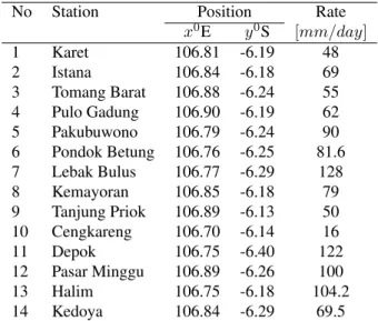
We chose area of Jakarta, the capital of Indonesia and surrounding as the study case with area approximately 900[km2]. The data of the rainfall rate measurement were taken from 14 rain gauge stations on 13 January 2014 as presented in Table I. The first eleven data in Table I were collected from the Buletin BMKG, January 2014 [15]. The last
three data (Pasar Minggu, Halim, Kedoya) are cited from the official website of BMKG [16].
Table I. Sample data of rainfall rate
No Station Position Rate
x0 E y0 S [mm/day] 1 Karet 106.81 -6.19 48 2 Istana 106.84 -6.18 69 3 Tomang Barat 106.88 -6.24 55 4 Pulo Gadung 106.90 -6.19 62 5 Pakubuwono 106.79 -6.24 90 6 Pondok Betung 106.76 -6.25 81.6 7 Lebak Bulus 106.77 -6.29 128 8 Kemayoran 106.85 -6.18 79 9 Tanjung Priok 106.89 -6.13 50 10 Cengkareng 106.70 -6.14 16 11 Depok 106.75 -6.40 122 12 Pasar Minggu 106.89 -6.26 100 13 Halim 106.75 -6.18 104.2 14 Kedoya 106.84 -6.29 69.5 2.2 Hardware
The parallel algorithms were conducted in a computer cluster provided by Research Center for Informatics, Indonesian Institute of Sciences, with the following specifications;
—16 nodes
—2 processors per node, 4 cores per processor —Dual Intel Xeon E5-2609 2,4 GHz
—8 GB RAM DDR3-1600 —500 GB HD SATA
—Dual Gigabit interconnection —NVIDIA Tesla M2075 GPGPU —Linux (CentOS)
Moreover we only investigate the numerical computation with the working nodes up to 4 as the computation needs 25 cores.
2.3 Inverse Distance Weigthing
Inverse distance weighting (IDW) is one simplest conventional interpolator to estimate the precipitation distribution. This interpolator assumes that the nearby values will contribute more to the estimated (unknown) values than the distant observations [17]. Consequently, the measured points are always maximum than the surrounding (the intensity of rainfall around the measured points is always larger); this behaviour is known as a bull eye’s effect . Furthermore we will work on the algorithm of IDW power 2 under assumption that all the measured data give influences to the unknown points, even though the measured data are far away from the unknown points. Basically, IDW works
by a weight function that is functioned of distance between the unknown points and the measured points (square of distance is used for IDW power 2). For given a set of N measured points,
(x1,x2,· · · ,xN), with corresponding precipitation
data, (u1, u2,· · · , uN), IDW estimates the
precipitation at the unknown points y by the following algorithm: for each y λj(y) = 1 |y−xj|2 u∗(y) = 1 PN j=1λj(y) N X j=1 (λj(y)uj)
The variable λj(y) denotes the weight function,
whileu∗(y)is the estimated precipitation at points
y 6= xj. The term of
1 PN
j=1λj(y)
is generally functioned to normalize the weight function, so that the weight function will be restricted in[0,1].
2.4 Ordinary Kriging
The best known geo-statistical interpolator is Ordinary Kriging [18]. This method is commonly used in geophysics community. It involves a stochastic pre-model to estimate the precipitation distribution. This interpolator is also based on weighted linear combination of the measured data as in IDW. In Ordinary kriging (OK), the weight function depends on the stochastic pre-model, so-called semivariogram model. The semivariogram model is chosen according to the experimental semivariogram computed from the measured data. It is a function of distance between two points. The best fit model is chosen as the empirical semivariogram. It could be one of the spherical, exponential or gaussian function. Meanwhile, the experimental semivariogram,γij, is
defined mathematically by the following expression:
γij = 1 2N(h) N(h) X n=1 E |un−un+h|2 (1)
in which N(h) denotes the number of points separated by the same distance h. If the empirical semivariogram has been chosen, we first compute the pre-model as below,
˜ γij = ˜γ(|xi−xj|) M= ˜ γ11 · · · γ˜1N 1 .. . . .. ... ... ˜ γN1 · · · γ˜N N 1 1 · · · 1 0
then the estimation of the precipitation is then computed by the following algorithm:
for each y ˜ γi0 = ˜γ(xi−y) λ(y) = λ1(y) .. . λN(y) µ =M−1· ˜ γ10 .. . ˜ γN0 1 u∗(y) = N X j=1 (λj(y)uj)
The function˜γijis a function chosen as the empirical
semivariogram model. The variableµinside matrix
M denotes the estimation error for each unknown point, which we will not discuss further in this paper.
3. PARALLEL ALGORITHMS
We propose two parallel algorithms of precipitation distribution based on Inverse distance weighting and Ordinary Kriging. The proposed parallel algorithms use single instruction multiple data (SIMD) construction. Spatial data is arranged in 2D manner. Let us assume the algorithms usesℓ = p2
cores. Then, the spatial domain is subdivided into
ℓ2D-subarea. Each core is given an index numberi
from0toℓ−1as shown in Figure 5 and computes the precipitation for subarea i. To simplify the parallel algorithms we divide the grid of the x−coordinate and y−coordinate with the same value. In other words, the area is divided quadratically, so we choose square numbers for the number of cores. We executed the parallel algorithms for both methods with 1, 4, 9, 16, and 25 cores.
Basically the parallel algorithms for IDW and OK are similar. The first step of the parallel algorithms for both methods is sharing the measured points and its precipitation data. Then, each core computes locally the estimated data of the unknown points. One additional step in parallel version for OK is that it needs pre-computation for computing matrix
M−1 before the local computation. As the matrix
is a function of distance between two measured points, there will be problematic when the number of measured points are getting larger. The numerical computation of the inverse matrix will be very costly, then it should be in parallel computing as suggested by [9]. Nevertheless, in this paper we do not apply a
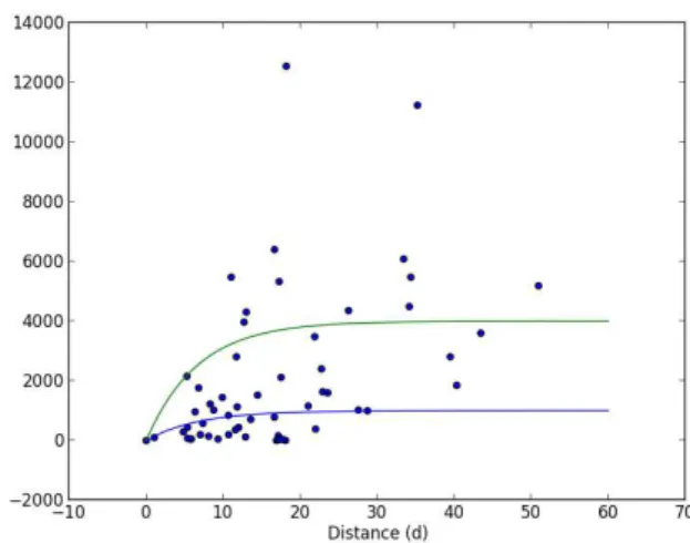
Figure 2. The experimental semivariogram model (dots) and empirical semivariogram models (solid line). The blue line
shows the exponential model withS = 1000andR = 20. The green line shows the exponential model withS = 4000and
R= 20.
Figure 1. The 2D spatial data is subdivided intoℓ = p2
subareas indexed by0toℓ−1.
parallel algorithm in computing the inverse matrix as our measured points are few. We use a numpy library in Python for computing the inverse matrix.
4. RESULTS AND ANALYSIS
We computed the semivariogram model from the measured data and then we find the best fit empirical
model. The experimental semivariogram is shown in Figure 2 together with the empirical semivariogram. According to the plots the covariance between the measured points are quite robust. Consequently, it is difficult to choose the best empirical model which represents the behaviour of the sample data. Nevertheless, we choose exponential model as the empirical semivariogram with the sill S = 4000
and the range R = 20. Sill is the maximum variance and range is the distance after which the correlation is zero. The empirical semivariogram model is formulated by ˜ γ(d) =S 1−exp −3d R
withdis the distance in [km].
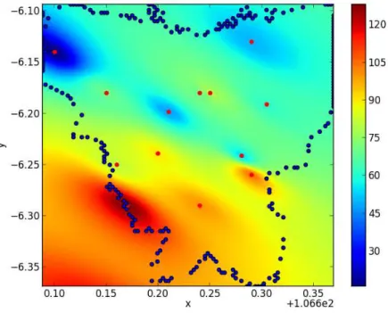
Both methods generally give similar spatial rainfall distribution. We show the results in the density plots in Figure 4. The bull’s eye effect could be observed in the spatial rainfall distribution by IDW.
We compare the time consumption for the numerical computation of IDW and OK. We also observe the time consumption of the algorithms with increasing number of the points/ cells. It is also presented in Table II.
Tabel II shows that the computation time for OK is longer than IDW approximately up to23%. This
Figure 3. The upper plot is the spatial rainfall distribution computed by Ordinary Kriging and the lower plot is the spatial rainfall distribution computed by Ordinary Kriging. The red-dots show the measured points and the blue-dots form the boundary of Jakarta area.
Table II. Computation time using serial algorithm of IDW and OK
Cell size [m2
] Number of cells Computation time[s]
IDW OK 1000x1000 2.85E+3 0.61 0.74 500x500 1.14E+4 2.39 2.93 250x250 4.56E+4 9.85 11.66 100x100 2.85E+5 59.46 73.23 50x50 1.14E+6 244.83 295.23 10x10 2.85E+7 5994.36 7191.68
is understandable as the weight function for OK’s algorithm is not as simple as IDW. It needs a
prior computation for the functionγ˜i0 in each loop.
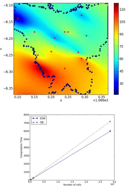
In addition we observe that the computation time (Comp.time) is linearly increasing with the number of the cells ans is inversely proportional to the cell size (see Figure 4);
Comp.time∼#cells∼ 1 cell size
In the parallel computations, we analyze the time consumption for IDW and OK’s algorithms with increasing number of cores (see Table III). As we do the computation in multi-cores we average the computation time from all cores. The result
Figure 4. Comparison of the computation time of the serial algorithm of IDW and OK.
is described in Figure 5. From the five different numbers of cores, the computation time shows an exponential decay, therefore we approximate their behaviour by exponential fitting (see Figure 5).
Table III. Computation time using parallel algorithm of IDW and OK with cell size of
100x100[m2 ]
#cores Computation time[s] Speed up
IDW OK IDW OK 1 59.46 73.23 1.00 1.00 4 15.09 18.14 3.94 3.98 9 6.72 8.07 8.84 8.94 16 3.78 4.55 15.71 15.88 25 2.56 3.05 23.21 23.65
From the exponential fitting, the time consumption (denoted byT(ℓ)) for IDW’s algorithm computation is decaying exponentially by the following formula;
T(ℓ) = 93.68e−0.52ℓ+ 3.96
Meanwhile OK’s algorithm decays by the formula below;
T(ℓ) = 116.63e−0.53ℓ+ 4.77
The values of 0.52 in IDW and 0.53 in OK are their decay factor. The larger the factor, the faster the computation time decreases.
Moreover we also evaluate the performance of the parallel algorithms by measuring speed up of both algorithms (see Table III). Speedup of a parallel computation is defined as the ratio between the sequential time and the parallel time to solve the same problem. We present the speed up curve in Figure 5. The speed up of both IDW and OK parallel algorithms are approximately the same. They are near ideal (linear) speed-up. It shows that
Figure 5. The blue lines represent the computation time and the red lines present the speed up of both parallel algorithms with respect to the number of computer cores. The solid line corresponds to IDW and the dashed-line corresponds to OK.
the additional computer cores are effectively used by both algorithms in the SIMD environment. The inefficiency must be caused by the inter-processor communication and synchronization in the computer cluster. This result agrees well to the study of [11] which also obtained near linear speed-up.
5. CONCLUSIONS
This paper investigated the parallel algorithms of Inverse Distance Weighting and Ordinary Kriging. These two algorithms were implemented to compute the spatial rainfall distribution. The computation time of Ordinary Kriging takes longer time up to 23% than Inverse Distance Weighting. This is understandable as the weight function of Ordinary Kriging needs a multiplication matrix in the algorithm. Nevertheless, our proposed parallel algorithms efficiently reduce the computational time and the additional computer cores in the computation is effectively used by the parallel algorithms in the SIMD architecture. One limitation of our proposed parallel algorithms is that the number of cores are restricted by square numbers.
The time consumption for the parallel algorithms are exponentially decaying with the number of working cores. The decay factor is 0.52 for IDW and 0.53 for OK. This concludes that the parallel algorithm of OK reduces a little faster than IDW. For a large measured data, the computation of inverse matrix in the algorithm of OK might be very costly. Consequently, the parallel algorithm of OK presented in this paper might need to be improved.
Acknowledgment
We acknowledge to Research Center for Informatics, Indonesian Institute of Sciences (LIPI) for the high performance computing facilities, http://grid.lipi.go. id.
Daftar Pustaka
[1] M. C. Acreman, “A simple stochastic model of
hourly rainfall for farnborough, england,”Hydrological
Sciences, vol. 35, no. 2, pp. 119–148, 1990.
[2] K. J. Beven, “On hypothesis testing in hydrology,”
Hydrological Process, vol. 15, no. 9, pp. 1655–1657, 2001.
[3] S. H. Roosta, Parallel Processing and Parallel
Algorithm, Theory and Computation. Springer-Verlag, 2000.
[4] N. Khorsandi, M. H. Mahdian, E. Pazira, D. Nikkami,
and H. Chamheidar, “Comparison of different
interpolation methods for investigating spatial
variability of rainfall erosivity index,”Pol. J. Environ. Stud., vol. 21, no. 6, pp. 1659–1666, 2012.
[5] A. D. Piazza, F. L. Conti, L. Noto, F. Viola, and G. L. Loggia, “Comparative analysis of different techniques for spatial interpolation of rainfall data to create a serially complete monthly time series of precipitation for sicily, italy,”International Journal of Applied Earth Observation and Geoinformation, vol. 13, no. 3, pp. 396–408, 2011.
[6] Z. P. Liu, M. A. Shao, and Y. Q. Wang, “Large-scale spatial interpolation of soil ph across the loess plateau,
china,”Environment Earth Sci, vol. 69, pp. 2731–2741,
2013.
[7] G. Mei, “Evaluating the power of gpu acceleration
for idw interpolation algorithm,” The Scientific World
Journal, 2014.
[8] K.E.Kerry and K.A.Hawick, “Kriging interpolation on
high-performance computers,” in Proceeding of the
International Conference and Exhibition on
High-Performance Computing and Networking Europe, 1998, pp. 429–438.
[9] W. Zhuo, Prabhat, C. Paciorek, C. Kaufman, and W. Bethel, “Parallel kriging analysis for large spatial
datasets,” in IEEE 11th International Conference on
Data Mining Workshop, 2011, pp. 38–44.
[10] J. Morrison, “Kriging in a parallel environment,”
Geomatics for informed decisions:GEOIDE, 2000. [11] M. Armstrong and R. Marciano, “Parallel spatial
interpolation,” in In Proceedings of the 11th
International Symposium on Computer Assisted Cartography, 1993, pp. 414–423.
[12] e. S.M.Bhandarkar, “Parallel computing of physical maps–a comparative study in simd and mimd parallelism,”J. Compu. Biol., vol. 3, no. 4, pp. 503–28, 1996.
[13] L. H. Jamieson, P. T. Mueller, and H. J. Siegel, “Fft algorithms for simd parallel processing systems,”
Journal of Parallel and Distributed Computing, vol. 3, pp. 48–71, 1986.
[14] R. H. Andrea Di Bias, Arun Jagota, “Optimizing
neural networks on simd parallel computers,”Parallel
Computing, vol. 31, no. 1, pp. 97–115, 2005.
[15] “Buletin BMKG, Analisis Hujan Bulan Januari 2014,” Stasiun Klimatologi Pondok Betung, Jl. Raya Kodam Bintaro no.82 Jakarta Selatan 12070, Tech. Rep., 2014.
[16] A. Zakir and M. Budiarti, Mungkinkah banjir besar
lagi di Jakarta. Available: http://bmkg.go.id/bmkg pusat/lain lain/artikel, 2014.
[17] M. Azpurua and K. D. Ramos, “A comparison of spatial interpolation methods for estimation of
average electromagnetic field magnitude,”Progress In
Electromagnetics Research M, vol. 14, pp. 135–145, 2010.
[18] U. Haberlandt, Flood Risk Assessment and
Management. Springer Science+Business Media B.V., 2011, ch. Interpolation of Precipitation for Flood Modelling, pp. 35–52.