Large Scale Decipherment for Out-of-Domain Machine Translation
Qing Dou and Kevin Knight Information Sciences Institute Department of Computer Science University of Southern California
{qdou,knight}@isi.edu
Abstract
We apply slice sampling to Bayesian de-cipherment and use our new dede-cipherment framework to improve out-of-domain machine translation. Compared with the state of the art algorithm, our approach is highly scalable and produces better results, which allows us to decipher ciphertext with billions of tokens and hundreds of thousands of word types with high accuracy. We decipher a large amount of monolingual data to improve out-of-domain translation and achieve significant gains of up to 3.8 BLEU points.
1 Introduction
Nowadays, state of the art statistical machine trans-lation (SMT) systems are built using large amounts of bilingual parallel corpora. Those corpora are used to estimate probabilities of word-to-word trans-lation, word sequences rearrangement, and even syntactic transformation. Unfortunately, as paral-lel corpora are expensive and not available for ev-ery domain, performance of SMT systems drops significantly when translating out-of-domain texts (Callison-Burch et al., 2008).
In general, it is easier to obtain in-domain mono-lingual corpora. Is it possible to use domain specific monolingual data to improve an MT system trained on parallel texts from a different domain? Some re-searchers have attempted to do this by adding a do-main specific dictionary (Wu et al., 2008), or mining unseen words (Daum´e and Jagarlamudi, 2011) us-ing one of several translation lexicon induction tech-niques (Haghighi et al., 2008; Koehn and Knight,
2002; Rapp, 1995). However, a dictionary is not al-ways available, and it is difficult to assign probabil-ities to a translation lexicon.
(Ravi and Knight, 2011b) have shown that one can use decipherment to learn a full translation model from non-parallel data. Their approach is able to find translations, and assign probabilities to them. But their work also has certain limitations. First of all, the corpus they use to build the translation sys-tem has a very small vocabulary. Secondly, although their algorithm is able to handle word substitution ciphers with limited vocabulary, its deciphering ac-curacy is low.
The contributions of this work are:
• We improve previous decipherment work by in-troducing a more efficient sampling algorithm. In experiments, our new method improves de-ciphering accuracy from 82.5% to 88.1% on (Ravi and Knight, 2011b)’s domain specific data set. Furthermore, we also solve a very large word substitution cipher built from the English Gigaword corpus and achieve 92.2% deciphering accuracy on news text.
• With the ability to handle a much larger vocab-ulary, we learn a domain specific translation ta-ble from a large amount of monolingual data and use the translation table to improve out-of-domain machine translation. In experiments, we observe significant gains of up to 3.8 BLEU points. Unlike previous works, the translation table we build from monolingual data do not only contain unseen words but also words seen in parallel data.
2 Word Substitution Ciphers
Before we present our new decipherment frame-work, we quickly review word substitution decipher-ment.
Recently, there has been an increasing interest in decipherment work (Ravi and Knight, 2011a; Ravi and Knight, 2008). While letter substitution ciphers can be solved easily, nobody has been able to solve a word substitution cipher with high accuracy.
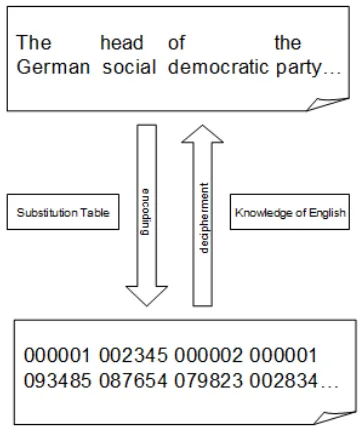
[image:2.612.94.274.336.551.2]As shown in Figure 1, a word substitution cipher is generated by replacing each word in a natural lan-guage (plaintext) sequence with a cipher token ac-cording to a substitution table. The mapping in the table is deterministic – each plaintext word type is only encoded with one unique cipher token. Solv-ing a word substitution cipher means recoverSolv-ing the original plaintext from the ciphertext without know-ing the substitution table. The only thknow-ing we rely on is knowledge about the underlying language.
Figure 1: Encoding and Decipherment of a Word Substi-tution Cipher
How can we solve a word substitution cipher? The approach is similar to those taken by cryptana-lysts who try to recover keys that convert encrypted texts to readable texts. Suppose we observe a large cipher stringfand want to decipher it into Englishe. We can follow the work in (Ravi and Knight, 2011b) and assume that the cipher stringf is generated in the following way:
• Generate English plaintext sequence e =
e1, e2...enwith probability P(e).
• Replace each English plaintext tokenei with a cipher tokenfiwith probabilityP(fi|ei).
Based on the above generative story, we write the probability of the cipher stringf as:
P(f)θ =
∑
e
P(e)·
n
∏
i
Pθ(fi|ei) (1)
We use this equation as an objective function for maximum likelihood training. In the equation,P(e)
is given by an ngram language model, which is trained using a large amount of monolingual texts. The rest of the task is to manipulate channel prob-abilitiesPθ(fi|ei) so that the probability of the ob-served textsP(f)θ is maximized.
Theoretically, we can directly apply EM, as pro-posed in (Knight et al., 2006), or Bayesian decipher-ment (Ravi and Knight, 2011a) to solve the prob-lem. However, unlike letter substitution ciphers, word substitution ciphers pose much greater chal-lenges to algorithm scalability. To solve a word sub-stitution cipher, the EM algorithm has a computa-tional complexity of O(N ·V2 ·R) and the com-plexity of Bayesian method isO(N ·V ·R), where V is the size of plaintext vocabulary, N is the length of ciphertext, and R is the number of iterations. In the world of word substitution ciphers, both V and N are very large, making these approaches impracti-cal. (Ravi and Knight, 2011b) propose several mod-ifications to the existing algorithms. However, the modified algorithms are only an approximation of the original algorithms and produce poor decipher-ing accuracy, and they are still unable to handle very large scale ciphers.
To address the above problems, we propose the following two new improvements to previous deci-pherment methods.
• We apply slice sampling (Neal, 2000) to scale up to ciphers with a very large vocabulary.
The new improvements allow us to solve a word substitution cipher with billions of tokens and hun-dreds of thousands of word types. Through better approximation, we achieve a significant increase in deciphering accuracy. In the following section, we present details of our new approach.
3 Slice Sampling for Bayesian Decipherment
In this section, we first give an introduction to Bayesian decipherment and then describe how to use slice sampling for it.
3.1 Bayesian Decipherment
Bayesian inference has been widely used in natural language processing (Goldwater and Griffiths, 2007; Blunsom et al., 2009; Ravi and Knight, 2011b). It is very attractive for problems like word substitution ciphers for the following reasons. First, there are no memory bottlenecks as compared to EM, which has anO(N ·V2)space complexity. Second, priors encourage the model to learn a sparse distribution.
The inference is usually performed using Gibbs sampling. For decipherment, a Gibbs sampler keeps drawing samples from plaintext sequences accord-ing to derivation probabilityP(d):
P(d) =P(e)·
n
∏
i
P(ci|ei) (2)
In Bayesian inference, P(e) is still given by an ngram language model, while the channel probabil-ity is modeled by the Chinese Restaurant Process (CRP):
P(ci|ei) =
α·prior+count(ci, ei)
α+count(ei)
(3)
Whereprioris the base distribution (we set prior to C1 in all our experiments, whereCis the number of word types in ciphertext), and count, also called “cache”, records events that occurred in the history. Each sampling operation involves changing a plain-text tokenei, which has V possible choices, where
V is the plaintext vocabulary size, and the final sam-ple is chosen with probability ∑VP(d)
n=1P(d) .
3.2 Slice Sampling
With Gibbs sampling, one has to evaluate all possi-ble plaintext word types (10k—1M) for each sam-ple decision. This become intractable when the vo-cabulary is large and the ciphertext is long. Slice sampling (Neal, 2000) can solve this problem by au-tomatically adjusting the number of samples to be considered for each sampling operation.
Suppose the derivation probability for current sample isP(current s). Then slice sampling draws a sample in two steps:
• Select a thresholdT uniformly from the range {0, P(current s)}.
• Draw a new sample new s uniformly from a pool of candidates:{new s|P(new s)> T}.
From the above two steps, we can see that given a thresholdT, we only need to consider those samples whose probability is higher than the threshold. This will lead to a significant reduction on the number of samples to be considered, if probabilities of the most samples are belowT. In practice, the first step is easy to implement, while it is difficult to make the second step efficient. An obvious way to collect can-didate samples is to go over all possible samples and record those with probabilities higher thanT. How-ever, doing this will not save any time. Fortunately, for Bayesian decipherment, we are able to complete the second step efficiently.
According to Equation 1, the probability of the current sample is given by a language modelP(e)
and a channel model P(c|e). The language model is usually an ngram language model. Suppose our current sample current s contains English tokens
X,Y, andZ at positioni−1,i, andi+ 1 respec-tively. Letci be the cipher token at positioni. To obtain a new sample, we just need to change token
Y toY′. Since the rest of the sample stays the same, we only need to calculate the probability of any tri-gram1:P(XY′Z)and the channel model probabil-ity: P(ci|Y′), and multiply them together as shown in Equation 4.
P(XY′Z)·P(ci|Y′) (4)
1
In slice sampling, each sampling operation has two steps. For the first step, we choose a thresh-oldTuniformly between0andP(XY Z)·P(ci|Y). For the second step, there are two cases.
First, we notice that two types of Y′ are more likely to pass the thresholdT: (1) Those that have a very high trigram probability , and (2) those that have high channel model probability. To find can-didates that have high trigram probability, we build sorted lists ranked byP(XY′Z), which can be pre-computed off-line. We only keep the top K En-glish words for each of the sorted list. When the last itemYKin the list satisfiesP(XYkZ)·prior <
T, We draw a sample in the following way: set
A = {Y′|P(XY′Z) ·prior > T} and set B =
{Y′|count(ci, Y′) >0}, then we only need to sam-ple Y′ uniformly from A∪ B until Equation 4 is greater thanT.2
Second, what happens when the last item YK in the list does not satisfy P(XYkZ) ·prior < T? Then we always choose a wordY′randomly and ac-cept it as a new sample if Equation 4 is greater than
T.
Our algorithm alternates between the two cases. The actual number of choices the algorithm looks at depends on theK and the total number of possible choices. In different experiments, we find that when
K = 500, the algorithm only looks at 0.06% of all possible choices. WhenK = 2000, this further re-duces to 0.007%.
3.3 Deciphering with Bigrams
Since we can decipher with a bigram language model, we posit that a frequency list of ciphertext bigrams may contain enough information for deci-pherment. In our letter substitution experiments, we find that breaking ciphertext into bigrams doesn’t hurt decipherment accuracy. Table 1 shows how full English sentences in the original data are broken into bigrams and their counts.
Instead of doing sampling on full sentences, we treat each bigram as a full “sentence”. There are
2It is easy to prove that all other candidates that are not in
the sorted list and withcount(ci, Y′) = 0have a upper bound
probability: P(XYkZ)·prior. Therefore, they are ignored
whenP(XYkZ)·prior < T.
man they took our land . they took our arable land .
took our 2 they took 2
land . 2
man they 1 arable land 1
Table 1: Converting full sentences to bigrams
two advantages to use bigrams and their counts for decipherment.
First of all, the bigrams and counts are a much more compact representation of the original cipher-text with full sentences. For instance, after breaking a billion tokens from the English Gigaword corpus, we find only 29m bigrams and 58m tokens, which is only 1/17 of the original text. In practice, we fur-ther discard all bigrams with low frequency, which makes the ciphertext even shorter.
Secondly, using bigrams significantly reduces the number of sorted lists (from|V|2to2|V|) mentioned in the previous section. The number of lists reduces from|V|2 to2|V|because words in a bigram only
have one neighbor. Therefore, for any word W in a bigram, we need only2|V|lists (“words to the right of W” and “words to the left of W”) instead of|V|2
lists (“pairs of words that surround W”).
3.4 Iterative Sampling
Although we can directly apply slice sampling on a large number of bigrams, we find that gradually including less frequent bigrams into a sampling pro-cess saves deciphering time – we call this iterative sampling:
• Break the ciphertext into bigrams and collect their counts
• Keep bigrams whose counts are greater than a threshold α. Then initialize the first sample randomly and use slice sampling to perform maximum likelihood training. In the end, ex-tract a translation table T according to the final sample.
ci-pher token f, choose a plaintext token e whose
P(e|f)is the largest). Perform sampling again.
• Repeat untilα= 1.
3.5 Parallel Sampling
Inspired by (Newman et al., 2009), our parallel sam-pling procedure is described below:
• Collect bigrams and their counts from cipher-text and split the bigrams into N parts.
• Run slice sampling on each part for 5 iterations independently.
• Combine counts from each part to form a new count table and run sampling again on each part using the new table.3
4 Decipherment Experiments
In this section, we evaluate our new sampling algo-rithm in two different experiments. In the first ex-periment, we compare our method with (Ravi and Knight, 2011b) on their data set to prove correct-ness of our approach. In the second experiment, we scale up to the whole English Gigaword corpus and achieve a much higher deciphering accuracy.
4.1 Deciphering Transtac Corpus
4.1.1 Data
We split the Transtac corpus the same way it was split in (Ravi and Knight, 2011b). The data used to create ciphertext consists of 1 million tokens, and 3397 word types. The data for language model training contains 2.7 million tokens and 25761 word types.4 The ciphertext is created by replacing each English word with a cipher word.
We use a bigram language model for decipher-ment training. When the training terminates, a trans-lation table with probabilityP(c|e)is built based on the counts collected from the final sample. For de-coding, we employ a trigram language model using full sentences. We use Moses (Koehn et al., 2007)
3
Except for combining the counts to form a new count table, other parameters remain the same. For instance, each part i has its own prior set to C1
i, whereCiis the number of word types
in that part of ciphertext.
4
In practice, we replaced singletons with a “UNK” symbol, leaving around 16904 word types.
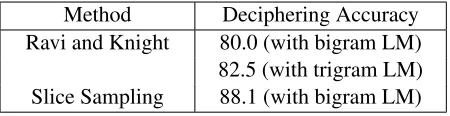
Method Deciphering Accuracy Ravi and Knight 80.0 (with bigram LM)
[image:5.612.315.540.57.115.2]82.5 (with trigram LM) Slice Sampling 88.1 (with bigram LM)
Table 2: Decipherment Accuracy on Transtac Corpus from (Ravi and Knight, 2011b)
Gold Decoded
man i’ve come to file a complaint against some people .
man i’ve come to hand a telephone lines some people .
man they took our land .
man they took our farm .
they took our arable land .
they took our slide door .
okay man . okay man . eighty donums . miflih donums .
Table 3: Sample Decoding Results on Transtac Corpus from (Ravi and Knight, 2011b)
to perform the decoding. We set the distortion limit to 0 and cube the translation probabilities. Essen-tially, Moses tries to find an English sequence e that maximizesP(e)·P(c|e)3
4.1.2 Results
We evaluate the performance of our algorithm by decipherment accuracy, which measures the per-centage of correctly deciphered cipher tokens. Table 2 compares the deciphering accuracy with the state of the art algorithm.
Results show that our algorithm improves the de-ciphering accuracy to 88.1%, which amounts to 33% reduction in error rate. This justifies our claim: do-ing better approximation usdo-ing slice sampldo-ing im-proves decipherment accuracy.
Table 3 shows the first 5 decoding results and compares them with the gold plaintext. From the ta-ble we can see that the algorithm recovered the ma-jority of the plaintext correctly.
4.2 Deciphering Gigaword Corpus
and has a much larger vocabulary compared with the Transtac corpus.
4.2.1 Data
We split the corpus into two parts chronologically. Each part contains approximately 1.2 billion tokens. We uses the first part to build a word substitution cipher, which is 10k times longer than the one in the previous experiment, and the second part to build a bigram language model.5
4.2.2 Results
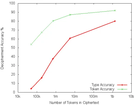
We first use a single machine and apply iterative sampling to solve a 68 million token cipher. Then we use the result from the first step to initialize our parallel sampling process, which uses as many as 100 machines. For evaluation, we calculate deci-phering accuracy over the first 1000 sentences (33k tokens).
[image:6.612.73.299.422.598.2]After 2000 iterations of the parallel sampling pro-cess, the deciphering accuracy reaches 92.2%. Fig-ure 2 shows the learning curve of the algorithm. It can be seen from the graph that both token and type accuracy increase as more and more data becomes available.
Figure 2: Learning curve for a very large word substitu-tion cipher: Both token and type accuracy rise as more and more ciphertext becomes available.
5
Before building the language model, we replace low fre-quency word types with an ”UNK” symbol, leaving 129k unique word types.
5 Improving Out-of-Domain Machine Translation
Domain specific machine translation (MT) is a chal-lenge for statistical machine translation (SMT) sys-tems trained on parallel corpora. It is common to see a significant drop in translation quality when trans-lating out-of-domain texts. Although it is hard to find parallel corpora for any specific domain, it is relatively easy to find domain specific monolingual corpora. In this section, we show how to use our new decipherment framework to learn a domain specific translation table and use it to improve out-of-domain translations.
5.1 Baseline SMT System
We build a state of the art phrase-based SMT system using Moses (Koehn et al., 2007). The baseline sys-tem has 3 models: a translation model, a reordering model, and a language model. The language model can be trained on monolingual data, and the rest are trained on parallel data. By default, Moses uses the following 8 features to score a candidate translation:
• direct and inverse translation probabilities • direct and inverse lexical weighting • phrase penalty
• a language model • a re-ordering model • word penalty
Each of the 8 features has its own weight, which can be tuned on a held-out set using minimum error rate training. (Och, 2003). In the following sections, we describe how to use decipherment to learn do-main specific translation probabilities, and use the new features to improve the baseline.
5.2 Learning a New Translation Table with
Decipherment
From a decipherment perspective, machine transla-tion is a much more complex task than solving a word substitution cipher and poses three major chal-lenges:
• Re-ordering of words
• Insertion and deletion of words
Fortunately, our decipherment model does not as-sume deterministic mapping and is able to discover multiple translations. For the reordering problem, we treat Spanish as a simple word substitution for French. Despite the simplification in the assump-tion, we still expect to learn a useful word-to-word lexicon via decipherment and use the lexicon to im-prove our baseline.
Problem formulation: By ignoring word
re-orderings, we can formulate MT decipherment prob-lem as word substitution decipherment. We view source languagef as ciphertext and target language
eas plaintext. Our goal is to decipherf into eand estimate translation probabilities based on the deci-pherment.
Probabilistic decipherment: Similar to solving
a word substitution cipher, all we have to do here is to estimate the translation model parametersPθ(f|e) using a large amount of monolingual data inf and
erespectively. According to Equation 5, our objec-tive is to estimate the model parameters so that the probability of source text P(f) is maximized.
arg max
θ
∑
e
P(e)·
n
∏
i
Pθ(fi|ei) (5)
Building a translation table: Once the sampling
process completes, we estimate translation probabil-ity P(f|e) from the final sample using maximum likelihood estimation. We also decipher from the re-verse direction to estimateP(e|f). Finally, we build a phrase table by taking translation pairs seen in both decipherments.
5.3 Combining Phrase Tables
We now have two phrase tables: one learnt from par-allel corpus and one learnt from non-parpar-allel mono-lingual corpus through decipherment. The phrase ta-ble learnt through decipherment only contains word to word translations, and each translation option only has two scores. Moses has a function to decode with multiple phrase tables, so we just need to add the newly learnt phrase table and specify two more weights for the scores in it. During decoding, if a source word only appears in the decipherment table,
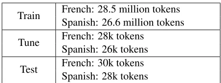
Train French: 28.5 million tokens Spanish: 26.6 million tokens
Tune French: 28k tokens Spanish: 26k tokens
[image:7.612.313.539.55.140.2]Test French: 30k tokens Spanish: 28k tokens
Table 4: Europarl Training, Tuning, and Testing Data
that table’s translation will be used. If a source word exists in both tables, Moses will create two separate decoding paths and choose the best one after taking other features into account. If a word is not seen in either of the tables, it is copied literally to the output.
6 MT Experiments and Results
6.1 Data
In our MT experiments, we translate French into Spanish and use the following corpora to learn our translation systems:
• Europarl Corpus (Koehn, 2005): The Europarl parallel corpus is extracted from the proceed-ings of the European Parliament and includes versions in 11 European languages. The cor-pus contains articles from the political domain and is used to train our baseline system. We use the 6th version of the corpus. After clean-ing, there are 1.3 million lines left for training. We use the last 2k lines for tuning and testing (1k for each), and the rest for training. Details of training, tuning, and testing data are listed in Table 4.
• EMEA Corpus (Tiedemann, 2009): EMEA is a parallel corpus made out of PDF documents from the European Medicines Agency. It con-tains articles from the medical domain, which is a good test bed for out-of-domain tasks. We use the first 2k pairs of sentences for tuning and testing (1k for each), and use the rest (1.1 million lines) for decipherment training. We split the training corpus in ways that no parallel sentences are included in the training set. The splitting methods are listed in Table 5.
ini-Comparable EMEA :
French: Every odd line, 8.7 million tokens Spanish: Every even line, 8.1 million tokens
Non-parallel EMEA:
French: First 550k sentences, 9.1 million tokens Spanish: Last 550k sentences, 7.7 million to-kens
Table 5: EMEA Decipherment Training Data
tialize our sampling process.
6.2 Results
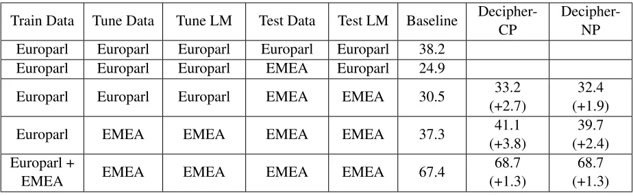
BLEU (Papineni et al., 2002) is used as a standard evaluation metric. We compare the following 3 sys-tems in our experiments, and present the results in Table 6.
• Baseline:Trained on Europarl
• Decipher-CP:Trained on Europarl +
Compa-rable EMEA
• Decipher-NP: Trained on Europarl +
Non-Parallel EMEA
Our baseline system achieves 38.2 BLEU score on Europarl test set. In the second row of Table 6, the test set changes to EMEA, and the baseline BLEU score drops to 24.9. In the third row, the base-line score rises to 30.5 with a language model built from EMEA corpus. Although it is much higher than the previous baseline, we further improve it by including a new phrase table learnt from domain specific monolingual data. In a real out-of-domain task, we are unlikely to have any parallel data to tune weights for the new phrase table. Therefore, we can only set it manually. In experiments, each score in the new phrase table has a weight of 5, and the BLEU score rises up to 33.2. In the fourth row of the table, we assume that there is a small amount of domain specific parallel data for tuning. With better weights, our baseline BLEU score increases to 37.3, and our combined systems increase to 41.1 and 39.7 respectively. In the last row of the table, we compare the combined systems with an even better baseline. This time, the baseline is given half of the EMEA tuning set for training and uses the other half
French Spanish P(f r|es) P(es|f r)
< < 0.32 1.00 h´epatique hep´atico 0.88 0.08 hep´atica 0.76 0.85 injectable inyectable 0.91 0.92
dl dl 1.00 0.70
> > 0.32 1.00 ribavirine ribavirina 0.40 1.00 olanzapine olanzapina 0.57 1.00 clairance aclaramiento 0.99 0.64 pellicul´ess recubiertos 1.00 1.00
pharmaco-cin´etique
farmaco-cin´etico 1.00 1.00
Table 7: 10 most frequent OOV words in the table learnt from non-parallel EMEA corpus
for weight tuning. Results show that our combined systems still outperform the baseline.
The phrase table learnt from monolingual data consists of both observed and unknown words. Ta-ble 7 shows the top 10 most frequent OOV words in the table learnt from non-parallel EMEA corpus. Among the 10 words, 9 have correct translations. It is interesting to see that our algorithm finds mul-tiple correct translations for the word “h´epatique”. The only mistake in the table is sensible as French word “pellicul´es” is translated into “recubiertos con pel´ıcula” in Spanish.
7 Conclusion and Future Work
Train Data Tune Data Tune LM Test Data Test LM Baseline Decipher-CP
Decipher-NP Europarl Europarl Europarl Europarl Europarl 38.2
Europarl Europarl Europarl EMEA Europarl 24.9
Europarl Europarl Europarl EMEA EMEA 30.5 33.2
(+2.7)
32.4 (+1.9)
Europarl EMEA EMEA EMEA EMEA 37.3 41.1
(+3.8)
39.7 (+2.4) Europarl +
EMEA EMEA EMEA EMEA EMEA 67.4
68.7 (+1.3)
[image:9.612.75.537.56.199.2]68.7 (+1.3)
Table 6: MT experiment results: The table shows how much the combined systems outperform the baseline system in different experiments. Each row has a different set of training, tuning, and testing data. Baseline is trained on parallel data only. Tune LM and Test LM specify language models used for tuning and testing respectively. Decipher-CP and Decipher-NP use a phrase table learnt from comparable and non-parallel EMEA corpus respectively.
8 Acknowledgments
This work was supported by NSF Grant 0904684. The authors would like to thank Philip Koehen, David Chiang, Jason Riesa, Ashish Vaswani, and Hui Zhang for their comments and suggestions.
References
Phil Blunsom, Trevor Cohn, Chris Dyer, and Miles Os-borne. 2009. A Gibbs sampler for phrasal syn-chronous grammar induction. In Proceedings of the Joint Conference of the 47th Annual Meeting of the ACL and the 4th International Joint Conference on Natural Language Processing of the AFNLP. Associa-tion for ComputaAssocia-tional Linguistics.
Chris Callison-Burch, Cameron Fordyce, Philipp Koehn, Christof Monz, and Josh Schroeder. 2008. Further meta-evaluation of machine translation. In Proceed-ings of the Third Workshop on Statistical Machine Translation. Association for Computational Linguis-tics.
Hal Daum´e, III and Jagadeesh Jagarlamudi. 2011. Do-main adaptation for machine translation by mining un-seen words. InProceedings of the 49th Annual Meet-ing of the Association for Computational LMeet-inguistics: Human Language Technologies. Association for Com-putational Linguistics.
Sharon Goldwater and Tom Griffiths. 2007. A fully Bayesian approach to unsupervised part-of-speech tag-ging. InProceedings of the 45th Annual Meeting of the Association of Computational Linguistics. Association for Computational Linguistics.
Aria Haghighi, Percy Liang, Taylor Berg-Kirkpatrick, and Dan Klein. 2008. Learning bilingual lexicons
from monolingual corpora. In Proceedings of ACL-08: HLT. Association for Computational Linguistics. Kevin Knight, Anish Nair, Nishit Rathod, and Kenji
Ya-mada. 2006. Unsupervised analysis for decipher-ment problems. InProceedings of the COLING/ACL 2006 Main Conference Poster Sessions. Association for Computational Linguistics.
Philipp Koehn and Kevin Knight. 2002. Learning a translation lexicon from monolingual corpora. In Pro-ceedings of the ACL-02 Workshop on Unsupervised Lexical Acquisition. Association for Computational Linguistics.
Philipp Koehn, Hieu Hoang, Alexandra Birch, Chris Callison-Burch, Marcello Federico, Nicola Bertoldi, Brooke Cowan, Wade Shen, Christine Moran, Richard Zens, Chris Dyer, Ondˇrej Bojar, Alexandra Con-stantin, and Evan Herbst. 2007. Moses: open source toolkit for statistical machine translation. In Proceed-ings of the 45th Annual Meeting of the ACL on Interac-tive Poster and Demonstration Sessions. Association for Computational Linguistics.
Philipp Koehn. 2005. Europarl: A parallel corpus for sta-tistical machine translation. InIn Proceedings of the Tenth Machine Translation Summit, Phuket, Thailand. Asia-Pacific Association for Machine Translation. Radford Neal. 2000. Slice sampling. Annals of
Statis-tics, 31.
David Newman, Arthur Asuncion, Padhrai Smyth, and Max Welling. 2009. Distributed algorithms for topic models.Journal of Machine Learning Research, 10. Franz Josef Och. 2003. Minimum error rate training
Kishore Papineni, Salim Roukos, Todd Ward, and Wei-Jing Zhu. 2002. Bleu: a method for automatic eval-uation of machine translation. InProceedings of the 40th Annual Meeting on Association for Computa-tional Linguistics. Association for Computational Lin-guistics.
Reinhard Rapp. 1995. Identifying word translations in non-parallel texts. InProceedings of the 33rd annual meeting on Association for Computational Linguistics. Association for Computational Linguistics.
Sujith Ravi and Kevin Knight. 2008. Attacking deci-pherment problems optimally with low-order n-gram models. InProceedings of the Conference on Empiri-cal Methods in Natural Language Processing. Associ-ation for ComputAssoci-ational Linguistics.
Sujith Ravi and Kevin Knight. 2011a. Bayesian infer-ence for Zodiac and other homophonic ciphers. In
Proceedings of the 49th Annual Meeting of the Asso-ciation for Computational Linguistics: Human Lan-guage Technologies. Association for Computational Linguistics.
Sujith Ravi and Kevin Knight. 2011b. Deciphering for-eign language. In Proceedings of the 49th Annual Meeting of the Association for Computational Linguis-tics: Human Language Technologies. Association for Computational Linguistics.
J¨org Tiedemann. 2009. News from OPUS – a collection of multilingual parallel corpora with tools and inter-faces. InRecent Advances in Natural Language Pro-cessing V, volume 309 ofCurrent Issues in Linguistic Theory. John Benjamins.
Hua Wu, Haifeng Wang, and Chengqing Zong. 2008. Domain adaptation for statistical machine translation with domain dictionary and monolingual corpora. In