Wave of chaos in a spatial eco-epidemiological system: Generating
realistic patterns of patchiness in rabbit-lynx dynamics
Ranjit Kumar Upadhyay
∗, P. Roy
†, C. Venkataraman
‡and A. Madzvamuse
§September 7, 2016
Abstract
In the present paper, we propose and analyse an eco-epidemiological model with diffusion to study the dynamics of rabbit populations which are consumed by lynx populations. Existence, boundedness, stability and bifurcation analyses of solutions for the proposed rabbit-lynx model are performed. Results show that in the presence of diffusion the model has the potential of exhibiting Turing instability. Numerical results (finite difference and finite element methods) reveal the existence of the wave of chaos and this appears to be a dominant mode of disease dispersal. We also show the mechanism of spatiotemporal pattern formation resulting from the Hopf bifurcation analysis, which can be a potential candidate for understanding the com-plex spatiotemporal dynamics of eco-epidemiological systems. Implications of the asymptotic transmission rate on disease eradication among rabbit population which in turn enhances the survival of Iberian lynx are discussed.
Keywords: Eco-epidemiological model, bifurcations analysis, diffusion-driven instability, Turing patterns
∗Corresponding author’s Email: [email protected], Phone No.: +91 326 2235482, Fax: +91 326 2296563. Department of Applied Mathematics, Indian School of Mines, Dhanbad, India.
†Department of Applied Mathematics, Indian School of Mines, Dhanbad, India.
‡University of Sussex, School of Mathematical and Physical Sciences, Department of Mathematics, University of Sussex, Brighton, BN1 9QH, United Kingdom
1
Introduction
European rabbit and Iberian lynx are closely associated species at broad spatial and temporal scales. Both originated in the Iberian peninsula and are linked to the Mediterranean environment of south-western Europe [6, 33, 49]. A long term monitoring program in Spain shows a remarkable decline in rabbit numbers in 2013. A similar trend has also been observed in the main areas inhabited by Iberian lynx [16]. The Iberian lynx, a vertebrate predator, has suffered severe population reduction in the 20th century and is now on the verge of extinction [20, 46]. The major decline of Iberian lynx is closely associated with sharp reduction in European rabbit (Oryctolagus cuniculus) abundance [52], caused by myxomatosis virus in 1950s and more recently Rabbit Hemorrhagic disease (RHD) [15]. European rabbit is a multifunctional species of the Iberian Mediterranean ecosystem, where it serves as prey for more than 28 predatory animals, alters the vegetation structure through seed dispersal and grazing. It also alters plant species composition, its urine have an effect on plant growth and soil fertility. It provides feeding resources for invertebrates and shelter for different species [15]. Continuous decline in biodiversity status and an acceleration of extinction rates have occurred in recent decades, leading to a growing international commitment toward conservation [61]. As species disappear and ecosystems are destroyed, our health, peace and security, jobs and economic prosperity are also hurt and very much affected. Saving species means a better world. The number of extinction and endangered species are growing but our understanding of the causes and dynamics of the extinction is still incomplete. This study is a small step towards understanding the extinction dynamics of lynx population due to the loss of its prey rabbit population. In our study, we will consider the interaction between Iberian lynx and European rabbits as unidirectional model, because lynx are extremely rare and rabbits are abundant and widely distributed [15]. Rabbits consistently account for more than 80% of the consumed biomass in the lynx diet and hence it shows that lynx is a rabbit specialist by necessity [19]. A specialist predator dies out when its favorite food is absent or is in short supply while the generalist predator switches to an alternate food option as when it faces difficulty to find its favorite preys [62]. Therefore, the specialist predator is more prone to extinction as compared to the generalist predator. The dramatic decline in rabbit populations, caused by RHD in 1980s, had a direct impact on lynx numbers. The Iberian lynx is currently at the edge of extinction because RHDV has wiped out the rabbits on which it depends. A new variant of RHDV has been detected since 2012 in most rabbit farms and in several wild population in Spain and Portugal [2, 13] suggesting that it has rapid spread throughout Iberian peninsula. Escaping through this extinction vortex is not possible using passive conservation measures and waiting for self recovery of populations. Recently, the issues and challenges for conserving the Iberian lynx population in Europe have been studied [54] and found that if the value of the disease transmission coefficient is reduced, the predator population (Iberian lynx) which is on the verge of extinction is saved.
In the field of eco-epidemiology, transmissible diseases are known to induce major behavioural changes in ecological systems. As a result, many models have been proposed and studied to investigate the mechanism of disease transmission [3, 11, 45, 54, 71]. Roy and Upadhyay [54] designed a spatial eco-epidemiological model with simple law of mass action and Holling type II functional response to understand the extinction dynamics of endangered lynx cat species. Fordham et al. [20] provided a framework for a next-generation model which simultaneously incorporates demography, dispersal, and biotic interactions into estimates of extinction risk under projected climate change. They used ecological niche models coupled to metapopulation simulations with source-sink dynamics to directly investigate the combined effects of climate change, prey availability and management intervention on the persistence of the Iberian lynx. Calvete [8] showed the impact of RHD on the dynamics of different classes of rabbit population (susceptible, infected, chronically infected and recovered class). Reddiex et al. [50] studied the impact of predation and RHD on population dynamics of rabbits. The results of such modelling efforts are helpful to predict the developmental tendencies of infectious diseases, to determine the key factors of the spread of infectious diseases and to deduce the optimum strategies for controlling and preventing the spread of diseases. Diffusion and transmission rates which are related to the reproduction rate
R0, have a great influence on the spread of the epidemics. Recent studies have shown that the incorporation
of spatial structure is crucial to eco-epidemiological modelling and theory [40]. Both population and disease dynamics exhibit similar properties with regards to pattern formation in space and time. Motivated from these facts we have studied the spatiotemporal pattern formation in a lynx-rabbit eco-epidemic system.
man-aging disease threats to animals and human populations. Recently Delibes-Mateos [16] studied the ecosystem effects of new variant RHDV on Iberia peninsula and show how this virus could threaten the conservation of endangered predators. In this work, we propose a new eco-epidemiological model considering disease in prey population (rabbit), which is consumed by predator population (Iberian lynx) and discuss the role of asymptotic transmission rate in the context of eco-epidemiology. Eco-epidemic research deals with diseases that spreads among interacting population, where epidemic and demographic aspects are merged together in one model. Apart from considering a different transmission function, we have included spatial variations while constructing the model. Spatial component of ecological interactions has been identified as an important factor of how the ecological communities are shaped. Very little attention has been paid so far to study the spatial three species eco-epidemiological model. Eco-epidemiological modelling using reaction-diffusion models can help us to un-derstand the distribution of species in both space and time. The main objective of this article is to study the bidirectional spread of epidemics through the wave of chaos phenomenon as well as studying the spatiotemporal epidemic dynamics. We also underpin the parameters that have important contributions to the dynamics and pattern formation of a realistic diffusive eco-epidemiological system. We also try to understand the spatial distribution of Iberian lynx population affected by deadly rabbit disease in prey population. We emphasize that the force of infection has an important contribution to the dynamics of this designed eco-epidemiological system. In this paper, we explore the value for predator conservation by addressing the bio-geographical relationship between a species of great conservation concern, the Iberian lynx, and its staple prey, the European rabbit. We have also tried to find major issues that can guide conservation action, and prioritize conservation-oriented research lines for the future.
Hence, the structure of this paper is as follows. In Section 2, we introduce the model system and its development. In Section 3, we present the detailed analysis of the non-spatial eco-epidemiological model. In this section, we study the boundedness of its solutions and characterise the equilibrium states thereby obtaining conditions under which the equilibrium states exist and are locally stable. It also contains the global stability and bifurcation analysis for the non-spatial model system. In Section 4, the conditions for diffusion-driven instability for the spatiotemporal model are derived and discussed. In Section 5, we present numerical simulation results in support of the theoretical findings in 1- and 2-dimensions. We conclude and discuss the results of our studies in Section 6. It is in this section that we interpret the ecological implications of our findings.
2
Model development: The eco-epidemiological system
In this paper, we design an eco-epidemiological model consisting of two populations:
1. The prey population, European rabbit, whose population density is denoted byN, the number of rabbit per unit designated area.
2. The predator population, Iberian lynx, whose population density is denoted byP, the number of lynx per unit designated area.
The following assumptions are made for formulating the basic differential equations:
Assumption 1. In the absence of the infective (I(t)) and predation (P(t)), the rabbit population grows according to a logistic law with intrinsic growth rate r ∈ ℜ+ and carrying capacity K ∈ ℜ+ such that dN
dt =
rN 1−N K
.
Assumption 2. In the presence of Infection, the total rabbit population is divided into two classes namely, susceptible rabbit population, denoted by S, and infected rabbit population, denoted byI. Therefore, at any time t, the total prey (i.e., rabbit) density is N(t) =S(t) +I(t) which is not constant but varies according to some growth law. For simplicity, we assume that the birth and death rate depends on the population size i.e.,
b(N) =rN and d(N) = rN2
K respectively and have logistic form [7]. Then the total population size satisfies
the logistic differential equation dN
dt =b(N)−d(N) =rN − rN2
K =rN 1− N K
,whereK >0 is the carrying capacity.
of the population and/or limitation of time [18]. c represents half saturation constant (see the derivation of a Holling type II functional response in prey-predator models). Biologically this constant lowers the infection rate due to spatial or social distribution and limitation of time. We assume that disease spreads among the prey only. Up to 90% of affected rabbits may die from the disease which progresses rapidly (death occurs approximately 1−3 days after infection (http://www.peteducation.com/article.cfm?c=18+1803&aid=1625)). Therefore we have considered no birth terms from I class. A typicalSI model with an open system of variable size can be written as:
dS dt =
S
N (b(N)−d(N))− βSI
N+c =rS 1− S+I
K
−SβSI+I+c =F(S, I), dI
dt = βSI
S+I+c−aI =G(S, I), (2.1)
where b, d: [0,∞)→(0,∞) are continuously differentiable functions. In this case, whenP = 0, no predation, the total rabbit population will satisfy the equation dN
dt =rS 1− S+I
K
−aI,whereadenotes the total death rate of the infected population due to disease-induced mortality and also due to natural death. The infected rabbits die after catching the infection and before they can reproduce as it is an extremely contagious and often fatal viral. Almost all adult die due to this disease while some young rabbits less than eight weeks old are less likely to become ill or die which are not capable of reproduction [68]. Therefore, we considered that only S
contributes to the net linear growth of the population.
Assumption 4. It is assumed that predators are not smart enough to distinguish between infected and susceptible rabbits, so that predator consumes the prey species (susceptible as well as infected) according to the Holling type II functional response [4]. If predators feed upon both susceptible rabbit (S) and infected rabbit (I) of a single species, then selectivity or preference of the predators to susceptible and infected preys plays significant role in the system dynamics [23]. In this case traditional type II functional response should be replaced by multiple-prey type II, which can be mathematically represented by ω1S/(S+b1I +c1) and
ω2S/(S+b1I+c1) for susceptible and infected rabbits, respectively [3, 9, 12]. The parameterb1measures the
selectivity/preference of the predator to infected rabbit over the susceptible one or vice-versa. If b1 >1, then
predators prefer infected preys. b1= 1 implies equal preference to susceptible and infected preys and 0< b1<1
means that predator prefer susceptible preys. However, in the absence of prey, the predator population die out exponentially. Assuming that predators (lynx) feed upon both the susceptible and infected preys with some preference to infected over the susceptible or vice-versa, and combining this with the systems (2.1), we formulate the required model given in (2.2). The model is basically a combination ofSImodel and Rosenzweig-MacArthur type predator-prey model
dS
dt =rS 1− S+I
K
−S+βSII+c− ω1SP
S+b1I+c1 :=Sg1(S, I, P),
dI dt =
βSI S+I+c−
ω2IP
S+b1I+c1 −aI :=Ig2(S, I, P),
dP dt =
ω3IP
S+b1I+c1 +
ω4SP
S+b1I+c1 −δP :=P g3(S, I, P),
(2.2)
with initial conditions S(0) > 0, I(0) > 0 and P(0) > 0. The interaction functions gi (i = 1,2,3) of the
model system (2.2) are continuous and have continuous partial derivatives on R3+:={(S, I, P)∈R3: S(0)>
0, I(0)>0, P(0)>0}.
All the model parametersr, K, β, c, c1, b1, ω1, ω2, ω3, ω4, aandδ are positive constants. The infected
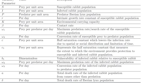
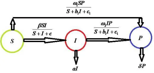
class also suffers loss through disease induced mortality apart from its natural death. Virus transmission causes loss of susceptible (S) and gain in infected (I) population (see Fig. 1). A brief description about variables and parameters used in the model system (2.2) is presented below in Table 2.
To proceed, we next introduce spatial variations to the model system (2.2). We assume that both prey and predator populations perform active movement inxandydirections which has been ignored in previous studies and is biologically relevant. Random movement of animals occurs because of various requirements like, search for better food, better opportunity for social interactions such as finding mates, etc [44]. Food availability and living conditions demand that these animals migrate to other spatial locations. In the proposed model, we have included diffusion terms to model the fact that the animal movements are random and uniformly distributed in all directions. We also assume that the three species diffuse with constant diffusion rates DS, DI and DP,
Variable/ Units Description Parameter
S Prey per unit area Susceptible rabbit population
I Prey per unit area Infected rabbit population
P Predator per unit area Predator Iberian lynx population
r Per day Intrinsic growth rate constant of susceptible rabbit population
K Prey per unit area Environmental carrying capacity
β Per day Contact rate
ω1 Prey per predator per day Maximum predation rate/search rate of the susceptible
rabbit population
ω4 Per day Conversion rate of susceptible prey to predator population
c Prey per unit area Half saturation constant which lowers the infection rate due to spatial or social distribution and limitation of time.
c1 Prey per unit area Represents the half saturation constant that measures
the extent to which the environment provides protection to susceptible and infected rabbit population.
b1 Dimensionless Vulnerability of infected rabbit relative to susceptible rabbit
ω2 Prey per predator per day Maximum predation rate of the infected rabbit population
ω3 Per day Conversion rate of the infected rabbit population
to predator population
a Per day Total death rate of the infected rabbit population
from causes other than predation
[image:5.595.85.554.146.423.2]δ Per day Total death rate of Iberian lynx population
Table 1: Model parameter values and their biological meanings.
concentration where the diffusion is no longer constant. If the predator and prey are confined to a fixed bounded domain Ω in R2, we led to consider the following reaction-diffusion system:
∂S
∂t −DS∇
2S =Sg
1(S, I, P), z∈Ω, t >0,
∂I
∂t−DI∇
2I =Ig
2(S, I, P), z∈Ω, t >0,
∂P
∂t −DP∇
2P =P g
3(S, I, P), z∈Ω, t >0,
(2.3)
with boundary conditions
(n· ∇)S= (n· ∇)I= (n· ∇)P= 0, for z∈∂Ω, t >0, (2.4)
and initial conditions
S(z,0) =S(0)>0, I(z,0) =I(0)>0, P(z,0) =P(0)>0,
(2.5)
wherez= (x, y)∈Ω = [0, L]×[0, L] and the kinetic functionsgi(S, I, P),i= 1,2,3 are defined in (2.2). In the
above, the vectornis an outward unit normal vector to the boundary∂Ω of the habitat Ω and the homogeneous
Figure 1: Schematic diagram for the eco-epidemic model (2.2).
3
Analysis of the Eco-epidemiological model
3.1
Analysis of non-spatial model system
It is necessary to investigate the temporal dynamics of the model system (2.2) before studying the spatiotemporal model system (2.3)-(2.5).
3.1.1 Boundedness of the system
The importance of boundedness in eco-epidemic system is not only interesting for mathematical reasons but also important from an ecological point of view. This result implies that none of the interacting species grow abruptly or exponentially for a long-time interval. The number/abundance of each species is bounded due to limited resources. We will now show that system (2.2) is uniformly bounded.
Theorem 3.1. If the following condition
ω2ω4−ω1ω3≥0 (3.1)
holds, all the non-negative solutions of model system (2.2)that start inR3
+ are uniformly bounded.
Proof. We define a function
h(t) =S(t) +I(t) +ω1
ω4
P(t). (3.2)
Then the time-derivative ofh(t) along the solutions of (2.2) is given by
dh dt =
dS dt +
dI dt +
ω1
ω4
dP
dt . (3.3)
Now for eachη >0, by substitutingS(t) andI(t) into equations (3.2) and (3.3) we obtain
dh
dt +ηh=S
η+r
1−KS
−
ω2−ω3
ω1
ω4
IP
S+b1I+c1 −
rSI
K −(a−η)I− ω1
ω4
(δ−η)P. (3.4)
Hence, it is easy to verify that under condition (3.1) we obtain
dh
dt +ηh≤S
η+r
1−KS
−(a−η)I−ωω1
4
(δ−η)P
≤K(r+η)
2
4r −(a−η)I− ω1
ω4
(δ−η)P. (3.5)
Now defining η <min(a, δ), then the right-hand side of the above inequality is bounded by K(r4+rη)2. We can thus findφ >0 such that dh
dt +ηh≤φ, which implies that
h(t)≤e−ηth(0) +φ
η(1−e
−ηt)≤max
h(0),φ
η
Moreover, for a suitable M independent of the initial conditions, we have limt→∞suph(t) ≤ φη =M. Thus
h(t) = S(t) +I(t) + ω1
ω4P(t) ≤M, hence all the species are uniformly bounded for any initial value in
R3
+ =
{(S, I, P) : 0< S≤η1, 0< I ≤η1, 0< P ≤η3}.
3.2
Linear stability analysis
In order to investigate the linear stability of the equilibrium points of system (2.2), first, we consider that system (2.2) can be separated into two independent subsystems. The first system is obtained by assuming the absence of the predators and can be written in the following form
dS dt =rS
1−SK+I
−S+βSII+c =Sg11(S, I), (3.7)
dI dt =
βSI
S+I+c −aI =Ig12(S, I). (3.8)
The second subsystem is obtained in the absence of the infected prey and takes the form
dS dt =rS
1−KS
−Sω1+SPc
1
:=Sg13(S, P), (3.9)
dP dt =
ω4SP
S+c1 −
δP :=P g14(S, P). (3.10)
Clearly, the interaction functions of systems (3.7)-(3.8) and (3.9)-(3.10) are continuous and have continuous partial derivatives on the state spaceR+. All the solutions of systems (3.7)-(3.8) and (3.9)-(3.10) which initiate
in a nonnegative domain are uniformly bounded as shown in Theorem 3.1.
It is well known that the Kolmogorov theorem is applicable to a two component dynamical system and guarantees the existence of either a stable equilibrium point or a stable limit cycle behaviour in the positive quadrant of the phase space of the system provided certain conditions are satisfied [62]. The amplitude and the period of the stable limit cycle oscillation depend on the values of the system parameters and strongly suggest that those natural systems which seem to exhibit a persistent pattern of reasonably regular oscillations possess a stable limit cycle [36]. When the Kolmogorov conditions are violated; one gets a repeller in the phase space.
Now we observe that the subsystem (3.7)-(3.8) is a Kolmogorov system under the condition
R01= βK
a(K+c) >1, (3.11)
and the subsystem (3.9)-(3.10) is a Kolmogorov system under the condition
R02= ω4K
δ(K+c1)
>1. (3.12)
From now on, we assume that subsystem (3.7)-(3.8) satisfies condition (3.11) and subsystem (3.9)-(3.10) satisfies condition (3.12). By applying the local stability analysis to the Kolmogorov systems (3.7)-(3.8) and (3.9)-(3.10) the following results are obtained.
3.2.1 Uniform steady states for the reduced two component systems
Let us consider theSIsystem given by (3.7)-(3.8). The first subsystem (3.7)-(3.8) has three nonnegative uniform steady states. The trivial uniform steady state is given by ¯E11 = (0,0). The disease-free equilibrium can be
shown to be given by ¯E12 = (K,0). The nontrivial equilibrium ¯E13= ( ¯S,I¯) which exists if and only if there is
a positive solution to the following set of equations
r
1−S¯+ ¯I
K
− ¯ βI¯
S+ ¯I+c = 0 = βS¯
¯
Solving the above system results in
¯
S=
a−p
(a−β)2B+ (a−β) (cr+K(a−β+r))
2(a−β)βr , (3.14)
¯
I= −(a−β)
2K
−(β(c−K) +a(c+K))r+ (a−β)√B
2βr , (3.15)
where
B=(a−β)2K2+ 2Kβ(c−K) +a(c+K)r+ (c+K)2r2.
Case 1: Whena−β >0, then
¯
S= a
−√B+ (cr+K(a−β+r))
2βr , (3.16)
¯
I= −(a−β)
2K−(β(c−K) +a(c+K))r+ (a−β)√B
2βr . (3.17)
The equilibrium point ¯E13 = ( ¯S,I¯) does not exist since there is no valid condition such that ¯S becomes
positive.
Case 2: Whena−β <0, then
¯
S=a
√
B+ (cr+K(a−β+r))
2βr , (3.18)
¯
I= −(a−β)
2K−(β(c−K) +a(c+K))r+ (a−β)√B
2βr . (3.19)
The existence criterion of the steady state population demands thatR01= a(βKK+c)>1.
Similarly, the uniform steady states corresponding to theSPsubsystem (3.9)-(3.10) are given by ˆE21= (0,0),
ˆ
E22= (K,0), and ˆE23= ( ˆS,Pˆ), where
ˆ
S= c1δ
ω4−δ and
ˆ
P = rω4c1(Kω4−δ(c1+K))
Kω1(δ−ω4)2 =
r Kω1(K−
ˆ
S)( ˆS+c1). (3.20)
Clearly, ˆE23 = ( ˆS,Pˆ) exists in the interior of the positive quadrant of the SP-plane provided the following
conditions are satisfied ifω4> δ andR02= (c1Kω+K4)δ >1.
3.2.2 Linear stability analysis of the non-spatial two component SI system
First, we study the local stability of the subsystem (3.7)-(3.8). The trivial equilibrium point ¯E11= (0,0) always
exists. For ¯E11 = (0,0), the eigenvalues are given by λ1 = r > 0 and λ2 = −a < 0. There is an unstable
manifold along the S-direction and a stable manifold along theI-direction. Therefore, the equilibrium point ¯
E11is a saddle point. The disease-free equilibrium point ¯E12= (K,0) exists on the boundary of the first octant.
For ¯E12, the eigenvalues are given by λ1=−r <0 andλ2 = βKK+−ca <0 if and only ifβK < a. Therefore the
equilibrium point ¯E12 is locally asymptotically stable providedβK < a, otherwise, it is a saddle point.
Let us consider the stability of the nontrivial equilibrium ¯E13 = ( ¯S,I¯). The variational matrix around the
endemic equilibrium point ¯E13 is given by
J∗=
J∗
11 J12∗
J∗ 21 J22∗
J11∗ =r
1−S¯+ ¯I
K
−rS¯
K −
βI¯(c+ ¯I) (c+ ¯I+ ¯S)2, J
∗ 12=−
rS¯ K −
βS¯(c+ ¯S) (c+ ¯I+ ¯S)2,
J21∗ =
βI¯(c+ ¯I) (c+ ¯I+ ¯S)2, J
∗
22=−a+
βS¯(c+ ¯S) (c+ ¯I+ ¯S)2,
and
Tr(J) = (J11∗ +J22∗) =−a−rS¯
K +
β( ¯S−I¯)
c+ ¯I+ ¯S +r
1−S¯K+ ¯I
,
Det(J) =J11∗J22∗ −J21∗J12∗ = βrS¯( ¯I
2
−I¯S¯+(K−2 ¯S)(c+ ¯S))+a(βI¯(c+ ¯I)K+r(c+ ¯I+ ¯S)2( ¯
I−K+2 ¯S))
K(c+ ¯I+ ¯S)2 .
If ¯E13 = ( ¯S,I¯) exists, i.e. if R01= a(KβK+c) >1 holds, then the eigenvalues of J have negative real parts and
hence the equilibrium point ¯E13 is stable.
Lemma 3.1. The equilibrium point E¯13= ( ¯S,I¯)is locally asymptotically stable in the interior of theSI-plane
whenever it exists.
3.2.3 Linear stability analysis of the non-spatial two component SP system
Similarly, the stability of the second subsystem (3.9)- (3.10) can be carried out as follows. The variational matrices of the subsystem (3.9)- (3.10) at ˆE21 and ˆE22 can be written as
J|ˆ
E21 =
r 0 0 −δ
and J|ˆ
E22 =
"
−r −Kω1
c1+K 0 −δ+ Kω4
c1+K
# .
Clearly ˆE21is a saddle point sincer >0 and−δ <0. Hence there is a locally stable manifold in theP-direction
and with a locally unstable manifold in the S-direction. Similarly, the eigenvalues of ˆE22 are −r < 0 and
−δ+ Kω4
c1+K. So, ˆE22 is locally asymptotically stable if and only if
Kω4
c1+K < δ. Finally, the variational matrix of the subsystem (3.9)-(3.10) at the positive equilibrium point ˆE23can be written in the form
J|ˆ
E23=
J11 J12
J21 J22
,
where
(
J11= ωδr4
1−c1
K
ω4+δ
ω4−δ
, J12=−δωω41,
J21= −δ(c1+KωK)r1+Krω4, and J22= 0.
Therefore, it is easy to verify that the eigenvalues ofJ satisfy the relations
ˆ
λ1+ ˆλ2=
δr ω4
1−c1
K ω
4+δ
ω4−δ
, and ˆλ1λˆ2=
δr ω4
−δ(c1+K) +Kω4
K . (3.21) Thus, if K c1
< ω4+δ ω4−δ
, (3.22)
holds then both eigenvalues have negative real parts and hence ˆE23is locally asymptotically stable in the interior
of the positive quadrant of theSP-plane, otherwise its an unstable point.
3.2.4 Uniform steady states for the three component non-spatial SIP system
In this section, the existence of the equilibrium points and local stability of the model system (2.2) are discussed. The system has five possible non-negative equilibrium points. The trivial equilibrium point E0 = (0,0,0)
always exists. The equilibrium point E1 = (K,0,0) exists on the boundary of the first octant. The
predator-free equilibrium point E2 = ( ¯S,I,¯ 0), where ¯S and ¯I are given by equations (3.18)-(3.19), exists provided
provided the condition (3.12) is satisfied. The nontrivial equilibrium (S∗, I∗, P∗) exists if and only if there is a
positive solution to the following set of equations
g1(S, I, P) =r
1−SK+I
−S+βII+c −S+ωb1P
1I+c1
= 0, (3.23)
g2(S, I, P) =
βS S+I+c−
ω2P
S+b1I+c1 −
a= 0, (3.24)
g3(S, I, P) =
ω3I
S+b1I+c1
+ ω4S
S+b1I+c1 −
δ= 0. (3.25)
Now, from equation (3.24), solving for P we have
P = (c1+b1I+S)(βS−a(c+I+S)) (c+I+S)ω2
. (3.26)
Substituting equation (3.26) into equation (3.23) and simplifying equation (3.25), we obtain the following system of nonlinear algebraic equations
f(S, I) =K(a(c+I+S)−Sβ)ω1−(r(c+I+S)(I−k+S) +IKβ)ω2= 0, (3.27)
g(S, I) = (c1+b1I+S)δ−Sω4−Iω3= 0. (3.28)
From equation (3.27) we note the following: whenI(t)−→0 thenS(t)−→Sa ast−→ ∞, where Sa is the
positive root of the quadratic polynomial
p2S2+p1S+p0= 0, (3.29)
with coefficients
p0=cK(aω1+rω2)>0, p1=K(a−β)ω1+ (−c+K)rω2, p2=−rω2<0.
This implies that there is exactly one positive root for the quadratic equation (3.29) irrespective of the sign of
p1. From equation (3.27) we have that
dS dI =−
∂f ∂I ∂f ∂S
=A1
B1
, (3.30)
where
A1=−aKω1+ (r(c+ 2I−K+ 2S) +Kβ)ω2, (3.31)
B1=K(a−β)ω1−rω2(c+ 2I−K+ 2S). (3.32)
It is clear that
dS
dI >0 if eitherA1>0 andB1>0 orA1<0 andB1<0 holds. (3.33)
Also from (3.28), we note that when I(t)−→0 then S(t)−→Sb ast−→ ∞, whereSb= ωc31−δδ.We note that
Sb>0 if the first inequality given byω3> δholds. We also have
dS dI =−
∂g ∂I ∂g ∂S
=−A2
B2
(3.34)
where
A2=b1δ−ω3, and B2=δ−ω4. (3.35)
It follows then that
dS
dI <0 if either A2>0 andB2>0 orA2<0 andB2<0 holds. (3.36)
From the above analysis we note that two isoclines (3.27) and (3.28) intersect at a unique equilibrium point (S∗, I∗) if in addition to conditions (3.12), (3.33) and (3.36), the inequalityS
Knowing the values ofS∗ andI∗, the value ofP∗can be calculated from
P∗=(c1+b1I∗+S∗)(βS∗−a(c+I∗+S∗))
(c+I∗+S∗)ω2 . (3.37)
It must be noted that for P∗ to be positive, we must haveβS∗> a(S∗+I∗+c). This completes the existence
of E∗(S∗, I∗, P∗). From the above analysis the following preposition can be proved.
Proposition 3.1. If the following conditions holds
1. A1>0andB1>0 or A1<0 andB1<0.
2. A2>0andB2>0 or A2<0 andB2<0.
3. Sa< Sb, whereA1, B1;A2, B2 andSa, Sb are defined above.
Then the nontrivial equilibrium E∗(S∗, I∗, P∗)exists if (β−a)S∗−a(I∗+c)>0.
3.2.5 Linear stability analysis of the non-spatial three componentSIP system
Now, in order to investigate the local behaviour of the model system (2.2) around each of the equilibrium point, the variational matrixJ evaluated at each point (S, I, P) is computed as follows
J(E) =
a11 a12 a13
a21 a22 a23
a31 a32 a33
.
The entries of the matrix are
a11= r(K−I−2S)
K −
βI(c+I) (c+I+S)2 −
ω1P(c1+b1I)
(c1+b1I+S)2
,
a12=S
b1ω1P
(c1+b1I+S)2−Kr −(c(+c+I+S)Sβ)2
,
a13=−
Sω1
c1+b1I+S
, a21=I
β(c+I)
(c+I+S)2 +
P ω2
(c1+b1I+S)2
,
a22=−a+ βS(c+S)
(c+I+S)2 −
ω2P(c1+S)
(c1+b1I+S)2, a23=−
ω2I
c1+b1I+S,
a31=
P((c1+b1I)ω4−Iω3)
(c1+b1I+S)2
, a32=
P(−b1ω4S+ (c1+S)ω3)
(c1+b1I+S)2
,
a33=
Sω4+Iω3−(c1+b1I+S)δ
c1+b1I+S
.
We denote J(Ek) = J(E) valued atEk and a[k]
ij =aij withi = 1,2,3,j = 1,2,3 and k= 0,1,2,3. Now, in
order to study the local stability of system (2.2), the variational matrix of system (2.2) is computed at each of the above equilibrium points and then the eigenvalues are determined.
The variational matrix atE0 is
J(E0) =
r 0 0
0 −a 0
0 0 −δ
.
ForE0, the eigenvalues arer,−a,−δ. There is an unstable manifold along theS-direction and a stable manifold
along theIP-direction. Therefore, the equilibrium pointE0 is a saddle point.
The variational matrix atE1 is
J(E1) =
−r −cβK+K −r − Kω1
c1+K 0 −a+cβK+K 0
0 0 −δ+ Kω4
c1+K
The corresponding eigenvalues are−a+cβK+K, −r, −δ+ ω4K
K+c1. Therefore, the equilibrium pointE1 is locally asymptotically stable providedR01<1 andR02<1. AlsoE1 is a saddle point if at least one of the conditions
R01>1 orR02>1 holds.
The variational matrix at the predator-free equilibrium pointE2= ( ¯S,I,¯ 0) can be written as
J(E2) =
r(K−2 ¯S−I¯)
K −
βI¯(c+ ¯I) (c+ ¯I+ ¯S)2 S¯
h
−r K −
β(c+ ¯S) (c+ ¯I+ ¯S)2
i
− ω1S¯
(c1+ ¯S+b1I¯)
βI¯(c+ ¯I)
(c+ ¯I+ ¯S)2 −a+
βS¯(c+ ¯S)
(c+ ¯I+ ¯S)2 −
ω2I¯
c1+ ¯S+b1I¯
0 0 −δ+ ω3I¯+ω4S¯
c1+ ¯S+b1I¯
.
Clearly the equilibrium point E2 = ( ¯S,I,¯ 0) has the same stability properties as ¯E13 = ( ¯S,I¯) in the interior
positive coordinate of the SI-plane. However, the stability of the point E2 = ( ¯S,I,¯0) is determined by the
positive direction orthogonal to the SI-plane, i.e, theP-direction, depending on whether the eigenvalue
¯
λp=−δ+
ω3I¯+ω4S¯
c1+ ¯S+b1I¯
(3.38)
is negative or positive, respectively.
According to Lemma 3.1, both eigenvalues ¯λS and ¯λI have negative real parts, while the eigenvalue ¯λP will
be negative if and only if
ω3I¯+ω4S¯
c1+ ¯S+b1I¯
< δ. (3.39)
Therefore,E2= ( ¯S,I,¯ 0) is locally asymptotically stable provided condition (3.39) holds.
The variational matrix at the disease-free equilibrium pointE3= ( ˆS,0,Pˆ) is
J(E3) =
r−2rSˆ K −
c1ω1Pˆ
(c1+ ˆS)2 − ˆ
S−r K −
β c+ ˆS +
b1P ωˆ 1
(c1+ ˆS)2
−ω1Sˆ
c1+ ˆS
0 −a− ω2Pˆ
ˆ
S+c1 +
βSˆ
c+ ˆS 0
ω4c1Pˆ
(c1+ ˆS)2
ˆ
P((c1+ ˆS)ω3−b1Sωˆ 4)
(c1+ ˆS)2 0
.
Then the eigenvalues of J(E3) satisfy the relations ˆλS+ ˆλP = ˆλ1+ ˆλ2 and ˆλSλˆP = ˆλ1λˆ2, where ˆλ1 and ˆλ2
represent the eigenvalues ofJ( ˆE23) and satisfy (3.21). However, ˆλI =−a− ω2Pˆ
ˆ
S+c1 +
βSˆ
c+ ˆS, where ˆλS, ˆλI and ˆλP
represents the eigenvalues of J(E3) in the S, I and P directions respectively. Therefore, it is clear that the
eigenvalues ˆλS and ˆλP have negative real parts if and only if condition (3.22) holds. However the eigenvalue ˆλI
is negative if and only if the following condition holds respectively
R0=
βSˆ( ˆS+c1)
(a(c1+ ˆS) +ω2Pˆ)(c+ ˆS)
<1. (3.40)
Following Hsieh and Hsiao [31], the termR0= β ˆ
S( ˆS+c1)
(a(c1+ ˆS)+ω2Pˆ)(c+ ˆS) gives the disease basic reproduction number of the system. R0is defined as the expected number of offsprings a typical individual produces in its life-time or
in epizootiology, as the expected number of secondary infections produced by a single infective individual in a completely susceptible population during its entire infectious period [17]. IfR0<1, it implies that the infected
prey will become extinct and consequently the disease will be eradicated from the system. Actually,R0<1 is
a necessary condition for local stability ofE3 = ( ˆS,0,Pˆ). Thus,E3 = ( ˆS,0,Pˆ) is asymptotically stable if and
only if conditions (3.22) and (3.40) hold. WhenR0= 1 one of the eigenvalue ofE3becomes zero and it exhibit
Theorem 3.2. The constant positive steady state E∗(S∗, I∗, P∗)of system (2.2) is locally asymptotically stable
provided the following conditions hold
r≤(cI+∗(cI∗++I∗S)∗β)2, a≥
S∗(c+S∗)β
(c+I∗+S∗)2, (3.41)
b1<
(c1+S∗)ω3
S∗ω4 ,
ω3
ω4 ≤
b1, (3.42)
P∗<(c1+b1I∗+S∗)
2 r(c+I∗+S∗)2+K(c+S∗)β
b1K(c+I∗+S∗)2ω1
, (3.43)
a≥KS
∗(c+S∗)βω1+I∗ r(c+I∗+S∗)2+K(c+S∗)β ω2
K(c+I∗+S∗)2ω 1
, (3.44)
ω2≥ω1, a≥
S∗β((c+I∗)ω
1+ (c+S∗)ω2)
(c+I∗+S∗)2ω 2
. (3.45)
Proof. The model system (2.2) is linearised at E∗(S∗, I∗, P∗) to yield the stability matrix
J(E∗) =
a∗11 a∗12 a∗13
a∗21 a∗22 a∗23
a∗31 a∗32 a∗33
.
The entries of the matrix are
a∗ 11=
r(−I+K−2S∗)
K −
I∗(c+I∗)β
(c+I∗+S∗)2 −
(c1+b1I∗)P∗ω1
(c1+b1I∗+S∗)2
,
a∗12=S∗
−Kr −(c+(c+I∗S+∗)Sβ∗)2 +
b1P∗ω1
(c1+b1I∗+S∗)2
,
a∗13=−
S∗ω1
c1+b1I∗+S∗
, a21=I∗
(c+I∗)β
(c+I∗+S∗)2 +
P∗ω2
(c1+b1I∗+S∗)2
,
a∗22=−a+
S∗(c+S∗)β
(c+I∗+S∗)2 −
P∗(c
1+S∗)ω2
(c1+b1I∗+S∗)2
, a23=−
I∗ω 2
c1+b1I∗+S∗
,
a∗31=
P∗((c1+b1I∗)ω4−I∗ω3)
(c1+b1I∗+S∗)2 , a ∗ 32=
P∗(−b1S∗ω4+ (c1+S∗)ω3)
(c1+b1I∗+S∗)2 , a33= 0.
The characteristics equation ofE∗(S∗, I∗, P∗) is given by
λ3+A1λ2+A2λ+A3= 0, (3.46)
where
A1=−(a11+a22), (3.47)
A2= (a11a22−a12a21)−(a23a32+a13a31), (3.48)
A3= (a13a22−a12a23)a31+ (a11a23−a13a21)a32, (3.49)
A1A2−A3=A1(a11a22−a12a21) +a31(a11a13+a12a23) +a32(a22a23+a13a21). (3.50)
Now according to Routh-Hurwitz criterion E∗ is locally asymptotically stable if
A1>0, A3>0, A1A2−A3>0. (3.51)
Clearly from condition (3.41) we obtain that a11 < 0, a22 <0 and hence A1 >0. Now, if (3.42) and (3.43)
holds a31>0 ,a32>0 anda12<0, therefore the second term of A3 is positive. Moreover, it is easy to verify
that the first term A3 i.e. (a13a22−a12a23) will be positive if condition (3.44) holds. It can be easily shown
that the first and the second terms of A1A2−A3 are positive. However the third term ofA1A2−A3 will be
positive if (a22a23+a13a21) >0, which is satisfied provided condition (3.45) holds. Hence the model system
Example 3.1. For the following set of biologically realistic parameter values (used in numerical simulation)
r = 6.1, K = 100, β = 7.69, b1 = 3, ω1 = 0.5, c = 10, c1 = 48, ω2 = 4.5, a = 0.19008, ω3 = 0.9, and
ω4= 0.12, andδ= 0.14 the positive equilibrium pointE∗ = (48.003797,16.000168,153.545549) settles down to
an asymptotic state which is confirmed by the Routh-Hurwitz criterion (A1= 1.15116>0,A2= 6.42556>0,
A3= 0.592248>0,andA1A2−A3= 6.80459>0).
Biologically, it means that the equilibriumE∗will act as sink and will attracts nearby solutions att→ ∞.
3.3
Global stability of the
SI P
non-spatial model system
Theorem 3.3. Assuming that the positive equilibrium point E∗ = (S∗, I∗, P∗) is locally asymptotically stable.
Then it is a globally stable in the interior of the positive octant (i.e., Int R3+) provided that
3r
2K +
β(S∗+c)
2(η1+η2+c)(S∗+I∗+c) >
P∗
2
ω1(b1+ 2) +ω2k1
c1(S∗+b1I∗+c1)+
βI∗(k
1+ 2) +k1c
2c(S∗+I∗+c) , (3.52)
and
r
2K +
β(3S∗+c)
2(η1+η2+c)(S∗+I∗+c)
> βk1(I∗+c)
2c(S∗+I∗+c)+
P∗(ω
1b1+ω2k1+ 2ω2b1)
2c1(S∗+b1I∗+c1)
. (3.53)
where η1,η2 andη3 are defined inR3+={(S, I, P) : 0< S≤η1, 0< I ≤η1, 0< P ≤η3}
Proof. Consider the following positive definite Lyapunov function about the equilibrium point
V(t) =
S−S∗−S∗ln S
S∗
+k1
I−I∗−I∗lnI∗
I
+k2
P−P∗−P∗lnP∗
P
, (3.54)
where k1 andk2 are positive constants to be chosen suitably later on. Obviously, V is a continuous function
in the interior of R3+. Now, in order to investigate the global dynamics of the non-negative equilibrium point
E∗ = (S∗, I∗, P∗) of the model system, the derivative ofV with respect to time along the solution of the system
is computed as
dV dt = dV1 dt + dV2 dt + dV3 dt .
Simple algebraic manipulations yield
dV dt =−
r K−
βI∗
(S∗+I∗+c)(S+I+c)−
ω1P∗
(S+b1I+c1)(S∗+b1I∗+c1)
(S−S∗)2
+−r K −
β((S∗+c)−k
1(I∗+c))
(S+I+c)(S∗+I∗+c) +
P∗(ω
1b1+ω2k1)
(S+b1I+c1)(S∗+b1I∗+c1)
(S−S∗)(I−I∗)
−k1
βS∗
(S+I+c)(S∗+I∗+c)−
ω2b1P∗
(S∗+b1I∗+c1)(S+b1I+c1)
(I−I∗)2
+ k2((S∗+c1)ω3−ω4b1S∗)
(S+b1I+c1)(S∗+b1I∗+c1)−
ω2k1
(S+b1I+c1)
(I−I∗)(P−P∗)
+k2((ω4b1−ω3)I∗+ω4c1)−ω1(S∗+b1I∗)
(S∗+b1I∗+c1)(S+b1I+c1)
(S−S∗)(P−P∗).
Choosing k2= ω1(S
∗+b
1I∗)
(ω4b1−ω3)I∗+ω4c1 andk1=
k2((S∗+c1)ω3−ω4b1S∗)
ω2(S∗+b1I∗+c1) we have
dV dt ≤ −
r K −
βI∗
(S∗+I∗+c)(S+I+c)−
ω1P∗
(S+b1I+c1)(S∗+b1I∗+c1)
(S−S∗)2
−k1
βS∗
(S+I+c)(S∗+I∗+c)−
ω2b1P∗
(S∗+b1I∗+c1)(S+b1I+c1)
(I−I∗)2
+
−Kr −(βS((+S∗I++cc))(−Sk∗1+(II∗∗++c))c)+ P∗(ω1b1+ω2k1) (S+b1I+c1)(S∗+b1I∗+c1)
(S−S∗)2+ (I−I∗)2
2
=−
3r
2K +
β((S∗+c)−I∗(k1+ 2)−k1c)
2(S∗+I∗+c)(S+I+c) −
(ω1(b1+ 2) +ω2k1)P∗
2(S+b1I+c1+)(S∗+b1I∗+c1)
(S−S∗)2
−k1
r
2K+
β((3S∗+c)−k
1(I∗+c))
2(S+I+c)(S∗+I∗+c)−
(ω2(k1+ 2b1) +ω1b1)P∗
2(S+b1I+c1)(S∗+b1I∗+c1)
Sufficient conditions for dV
dt to be negative definite require that conditions (3.52) and (3.53) hold. This proves
the result.
3.4
Bifurcation analysis
Theorem 3.4. Assume that condition (3.40)holds, then system (2.2)has a Hopf bifurcation near the disease-free equilibrium point E3( ˆS,0,Pˆ)as the parameter value K passes through the critical valueKcr= c1ω(δ4+−ωδ4).
Proof. According to the variational matrix J(E3) at the disease-free equilibrium pointE3( ˆS,0,Pˆ), the
eigen-values for the equilibrium pointE3( ˆS,0,Pˆ) can be written as ˆλS,P =−B±
√
B2−4A
2 and ˆλI =−a−
ω2Pˆ
ˆ
S+c1 +
βSˆ c+ ˆS,
where
B= ˆλS+ ˆλP =
δr(K(ω4−δ)−c1(δ+ω4))
K(ω4−δ)ω4 ,
and
A=rδ
1−(c1Kω+K)δ
4
>0.
Now it has been shown that λI <0 if and only if condition (3.40) holds. However, the eigenvaluesλS and λP
are pure imaginary numbers forB= 0 orK=Kcr, so there is a neighbourhood aroundK=Kcrsuch thatλS
andλP can be written asλS,P =θ(K)±iθ1(K),whereθ(K) =δr(K(ωK4(−ωδ4)−−δc)1ω(4δ+ω4)) represents the real part of
λS andλP. Now since
h
dθ(K)
dK
i
K=Kcr
= c1δr(δ+ω4)
K2(ω
4−δ)ω4 6= 0. Therefore, system (2.2) has Hopf bifurcation near the disease-free equilibrium point at K=Kcr. This completes the proof.
Now since the predator-free equilibrium point E2 has two eigenvalues with negative real parts while the
third that is given by (3.38) is real and is negative depending on condition (3.39). Then, there is no possibility to have a Hopf bifurcation near this point.
Theorem 3.5. When β =β∗, then the equilibrium E3 will be transformed into a non-hyperbolic equilibrium,
and the system attains neither a saddle-node bifurcation nor a pitchfork bifurcation, but exhibits a transcritical bifurcation.
Proof. One of the eigenvalues ofJ(E3) will be zero if and only if detJ(E3) =−a[3]13a[3]22a[3]31 = 0,i.e. a[3]22 = 0,
since (a[3]13, a[3]31) 6= (0,0). This gives β = β∗ = (c+ ˆS)(a(c1+ ˆS)+ ˆP ω2)
ˆ
S(c1+ ˆS) . The other two eigenvalues are given by ˆ
λ± = a [3] 11 2 ± 1 2 q
(a[3]11)2+ 4a [3] 13a
[3]
31.We will denote ˆλ+ = ˆλ2 and ˆλ− = ˆλ3. Since a[3]13 <0 and a [3]
31 >0, the real
parts of ˆλ2 and ˆλ3 will be of the same sign as that ofa11[3]. Now, ifK < Kcr= c(1ω(δ4+−ωδ4)), thena[3]11 >0 and two
eigenvalues ofJ(E3) will be positive; hence the proof follows from Sotomayor [58].
Again if K > Kcr then a[3]11 < 0. In this case, Ω = (θ1, θ2, θ3)T, Υ = (0, ξ,0)T, where Ω and Υ
are the eigenvectors corresponding to the eigenvalue ˆλ1 = 0 of the matrices J(E3) and J(E3)T,
respec-tively, and θ1 = − ~2a[3]32
a[3]31
, θ2 = ~2, θ3 = ~2(a[3]32a
[3] 11−a
[3] 31a
[3] 12)
a[3]13a [3] 31
and ~2, and ξ are any two non-zero real numbers
[24, 58]. Now, ΥT[F
β(E3, β∗)] = 0, so the system does not experience any saddle-node bifurcations. Again,
ΥT[DF
β(E3, β∗)Ω] = ˆS2~2θ2 6= 0 and ΥT[D2Fβ(E3, β∗)(Ω,Ω)] 6= 0 where [DFβ(E3, β∗)] = (bij)3×3, with
b11 = 0, b12 = −Sˆ, b13 = 0, b21 = 0, b22 = ˆS, b23 = 0, b31 = 0, b32 = 0 and b33 = 0. D2F(E3, β∗) is
a 3×3×3 tensor. Thus, by the same theorem the system possesses a transcritical bifurcation [58]. Again, ΥT[D2F
β(E3, β∗)(Ω,Ω)]6= 0. Therefore, the system does not experience a pitchfork bifurcation.
Theorem 3.6. Assume that the conditions (3.41)-(3.44) hold. Then, system (2.2)exhibits a Hopf bifurcation near the positive equilibrium point E∗ as the parameter r passes through the critical valuerc provided that the
S∗ b1P∗ω1
(c1+b1I∗+S∗)2
− r
K −(c+S
∗)T
!
× I∗ (c+I∗)T+ P∗ω2 (c1+b1I∗+S∗)2
!
Q−I∗P∗ω2(−I∗ω3+ (c1+b1I∗)ω4)
(c1+b1I∗+S∗)3
!
< I∗P∗((c1+S∗)ω3−b1S∗ω4)
(c1+b1I∗+S∗)3
S∗ω1 (c+I∗)T+
P∗ω2
(c1+b1I∗+S∗)2
!
+ω2Q
!
(3.55)
where T =(S∗+Iβ∗+c)2 andQ=−a+S∗(c+S∗)T −
P∗(c1+S∗)ω2
(c1+b1I∗+S∗)2.
Proof. The characteristic equation of J(E∗) is given by λ3+A1λ2+A2λ+A3= 0, whereAi′s; i= 1,2,3 are
given in Theorem 3.2. It had been observed that conditions (3.41)-(3.44) guarantee thatAi>0;i= 1,2,3 for
all values of r.
Since the Hopf bifurcation near the positive equilibrium pointE∗of system (2.2) occurs if and only ifJ(E∗)
has two complex conjugate eigenvalues with the third eigenvalue real and negative such that there exists a constant parameter value, say rc, the necessary and sufficient conditions for Hopf bifurcation at r = rc are
A1>0, A3>0,ψ(rc) =A1(rc)A2(rc)−A3(rc) = 0 and dRe(drλ(r))
r=rc
6
= 0; whereλis a complex eigenvalue of
J(E∗).
So, by simplifyingψ(rc) =A1(rc)A2(rc)−A3(rc) and then equating it to zero we geta∗22(a∗11)2−N1a∗11−N2=
0 whereN1=a∗13a∗31+a∗12a∗21−a∗22
2 andN
2=a∗12(a∗21a∗22+a∗23a∗31) +a∗32(a∗22a∗23+a∗21a13∗ ), anda∗ij;i, j= 1,2,3
represents the elements ofJ(E∗). ObviouslyN
1<0 , while condition (3.55) guarantees thatN2<0. Therefore,
by solving the above second order equation we first obtain a∗ 11 = 2Na∗1
22 +
1 2a∗
22
p N2
1+ 4a∗22N2. Substituting
the value of a∗
11 in this equation and then solving for r we get that r=rc. Accordingly, for r =rc we have
A1A2=A3 and then the above characteristic equation can be written as
(λ2+A2)(λ+A1) = 0. (3.56)
For allλ, the roots are generally of the formλ1(r) =η1(r) +iη2(r),λ2(r) =η1(r)−iη2(r), andλ3(r) =−A1(r).
Now we shall prove the transversality condition dRe(λj(r))
dr
r=rc
6
= 0, j= 1, 2.
Substituting λ1(r) =η1(r) +iη2(r) into the characteristic equation and calculating the derivative, we have
K(r)η1′(r)−L(r)η2′(r) +M(r) = 0, and L(r)η1′(r) +K(r)η2′(r) +N(r) = 0,
where
K(r) = 3η12(r) + 2A1(r)η1(r) +A2(r)−3η22(r),
L(r) = 6η1(r)η2(r) + 2A1(r)η2(r),
M(r) =η12(r)A1′(r) +A2′(r)η1(r) +A3′(r)−A1′(r)η22(r),
N(r) = 2η1(r)η2(r)A1′(r) +A2′(r)η2(r).
Since L(rc)N(rc) +K(rc)M(rc) 6= 0, we have drd (Reλj(r))
r=rc =
h
LN+KM K2+L2
i
r=rc
6
= 0 and λ3 = −A1 6= 0.
Therefore, the transversality condition holds. This implies that a Hopf bifurcation occurs atr=rc and is
4
Analysis of spatial model system
4.1
Linear stability analysis of the
SI P
spatial model system
For the linear stability analysis of the spatiotemporal model system (2.3), it is perturbed with the following 2-dimensional spatiotemporal perturbations of the form
S =S∗+ǫ
1exp(λkt+i(kxx+kyy)) =S∗+ǫ1s1,
I=I∗+ǫ2exp(λkt+i(kxx+kyy)) =I∗+ǫ2i1,
P =P∗+ǫ
3exp(λkt+i(kxx+kyy)) =P∗+ǫ3p1,
(4.1)
where ǫ1,ǫ2 and ǫ3 are sufficiently small constants,kx and ky are the components of the wavenumberkalong
xandy directions respectively, andλk is the wavelength.
Theorem 4.1. Assume that the parameters in model system (2.3) satisfy conditions (3.41)-(3.45). Then the constant positive steady state E∗(S∗, I∗, P∗)of the spatiotemporal system is locally asymptotically stable.
Proof. The system is linearized about the non-trivial interior equilibrium pointE∗(S∗, I∗, P∗). The
character-istic equation of the linearized version of the spatiotemporal model system (2.3) is given by
(J−Dk2−λkI) s1, i1, p1T = 0, (4.2)
with
J =
a11 a12 a13
a21 a22 a23
a31 a32 a33
, and D=
DS 0 0
0 DI 0
0 0 DP
(4.3)
wherekis the wavenumber given byk2=k2
x+ky2andI is a 3×3 identity matrix. The entries of the variational
matrixJ are the same as those defined in Theorem 3.2. From (4.2) and (4.3), we get the characteristic equation
of the form
det(J−Dk2−λkI) =λ3
k+ρ1(k2)λ2k+λkρ2(k2) +ρ3(k2) (4.4)
where
ρ1(k2) =−tr(J−Dk2) =k2(DS+DI+DP) +A1,
ρ2(k2) =k4(DSDI +DSDP+DPDI)−k2(DS(a33+a22) +DI(a11+a33)
+DP(a11+a22)) +A2,
ρ3(k2) =−det(J−Dk2) =k6(DSDIDP) +k4(−DSDIa33−a22DSDP−a11DIDP)
+k2(D
S(a33a22−a23a32) +DI(a11a33−a13a31) +DP(a11a22−a12a21)) +A3.
(4.5)
In the above A1, A2 and A3 are as defined in (3.47)-(3.49). From assumptions (3.41)-(3.45), it follows that
ρ1(k2)>0, ρ2(k2)>0 andρ3(k2)>0. Algebraic manipulation of the expressionρ1(k2)ρ2(k2)−ρ3(k2) yields
B1k6+B2k4+B3k2+A1A2−A3, (4.6)
where
B1= (DS+DI)(DS+DP)(DI+DP)>0,
B2=−a11(DI+DP)(DI + 2DS+DP)−a22(DS+DP)(2DI+DS+DP)
−a33(DI+DS)(DI+DS+ 2DP)>0,
B3= (−(a22+a33)A1+ (a11a22−a12a21)−a31a13+a33a11)DS
+(−(a11+a33)A1+ (a11a22−a12a21)−a23a32+a33a22)DI)
+(−(a22+a11)A1+ (a11+a22)a33−a23a32+a13a31)DP)>0.
An application of the Routh-Hurwith criteria gives ℜ(λ(k)) < 0 if and only if ρ3(k2) > 0, ρ1(k2) > 0 and
ρ1(k2)ρ2(k2)−ρ3(k2)>0. Thus the constant positive steady stateE∗(S∗, I∗, P∗) of the spatiotemporal system
Remark 4.1. As a consequence of Theorem 3.2, under conditions (3.41)-(3.45), diffusion cannot destabilize the constant coexistence steady state E∗(S∗, I∗, P∗) of the system (2.3) and Turing instability cannot occur
in the vicinity of E∗(S∗, I∗, P∗). Hence system (2.3) will not have a non-constant positive steady state in
some neighborhood of E∗(S∗, I∗, P∗) under conditions (3.41)-(3.45). However, if any one of the conditions
(3.41)-(3.45) fails there is a possibility for the occurrence of Turing instability.
Example 4.1. For illustrative purposes, let us take the data set r= 6.1,K= 100,β= 7.69,ω1= 0.5,c= 10,
c1 = 48,ω2 = 4.5, a = 0.19008, ω3 = 0.9, and ω4 = 0.12,δ = 0.14. It can be shown that for this data set,
condition (3.41) fails since a22 = 0.520863>0 but condition (3.51) (A1 = 1.15116>0, A3 = 0.592248 >0,
A1A2−A3= 6.80459) still holds andE∗(S∗, I∗, P∗) is temporally stable. Furthermore,ρ3(k2) changes its sign
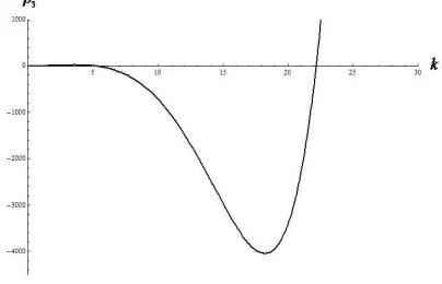
[image:18.595.217.419.322.452.2]as the wavenumber k varies as shown in Figure 2. In this case, Turing instability is possible. Accordingly, the system may eventually go to a non-constant positive steady state. Thus, the existence of a non-constant positive steady state may be possible when some of the conditions (3.41)-(3.45) fail.
Figure 2: The occurrence of Turing instability as the coefficient (ρ3) of the dispersion relation (4.4) becomes
negative for some range of wavenumberk.
4.2
Characterization of the diffusion-driven instability
The spatially homogeneous state will be unstable provided that at least one eigenvalue of the characteristic Eq. (4.4) is positive. It is clear that the homogeneous steady state E∗ is asymptotically stable if and only if
ρ1(0)>0,ρ3(0)>0 andρ1(0)ρ2(0)−ρ3(0)>0. But it will be driven to an unstable state by diffusion if any
of the conditions
ρ1(k2)>0, ρ3(k2)>0 and ρ1(k2)ρ2(k2)−ρ3(k2)>0, (4.7)
fail to hold. However, it can be easily seen that diffusion-driven instability cannot occur by contradicting
ρ1(k2)>0. SinceDS,DI,DP andk2are all positive, the inequalityρ1(k2)>0 always holds sinceA1>0 from
the stability condition of the interior equilibrium point in homogeneous state. Thus, the system is stable in the absence of diffusion, as a resultA1is always positive. Hence, we have to look for conditions which reverse the
sign of the other two conditions in Eq. (4.7). The expressions for ρ3(k2) and ρ1(k2)ρ2(k2)−ρ3(k2) are both
cubic functions ofk2 of the form
G(k2) =G3k6+G2k4+G1k2+G0, such that G3>0, G0>0.
The coefficient Gi (i = 0,1,2,3) for expression of ρ3(k2)>0 and ρ1(k2)ρ2(k2)−ρ3(k2)>0 are the same as
those given in the third Eq. of (4.5) and (4.6), respectively. For G(k2) to be negative for some positive real
number k26= 0, the minimum must be negative. This minimum occurs atk2=k2
c =
−G2+√G22−3G1G3
3G3 . Nowk
2
c
is real and positive if
Hence
Gmin=G(Kc2) =
2G3
2−9G1G2G3−2(G22−3G1G3)
3
2 + 27G2
3G0
27G2 3
.
Thus
G(kc2)<0, if 2G32−9G1G2G3−2(G22−3G1G3)
3
2 + 27G2
3G0<0. (4.9)
The conditions given in equations (4.8) and (4.9) are sufficient for the occurrence of diffusion-driven instability. The above results are summarised in the following theorem.
Theorem 4.2. The spatial model system (2.3) will undergo diffusion-driven instability at the homogeneous steady stateE∗ provided the following conditions are satisfied
G1<0 or (G2<0 and G22>3G1G3),
and
(G32+
27 2 G
2 3G0−
9
2G1G2G3)
2<(G2
2−3G1G3)3.
Proof. The proof directly follows from the above derivation.
4.3
Global stability of the
SI P
spatiotemporal model system
To establish the global stability of the positive steady stateE∗, first we recall the following result which can be
found in Wang [67].
Lemma 4.1. Let aandb be positive constants. Assume thatϕ, ψ∈C1[a,∞), ψ(t)≥0 andϕis bounded from
below. If ϕ′
≤ −bψ(t)andψ′
≤K∈[a,∞)for some constant K, then lim
t→∞ψ(t) = 0.
Hence, we can state the following result whose proof is given in Appendix A.
Theorem 4.3. The constant positive steady state E∗(S∗, I∗, P∗) of the spatial model system (2.3) is globally
asymptotically stable if the conditions for global stability for the non-spatial model (2.2) hold.
5
Numerical simulations
5.1
In the absence of diffusion
In this section, we present detailed numerical simulations of the model system (2.2) in the absence of diffusion. Our aim is to support our theoretical findings resulting from the study of the dynamic behavior of the model system.
The model system (2.2) is integrated using fourth-order Runge-Kutta method under different sets of pa-rameter values and different sets of initial conditions. It is observed that for the following hypothetical set of parameter values r = 6.1, K = 100, β = 7.69, b1 = 3, ω1 = 0.5, c = 10, c1 = 48, ω2 = 4.5, a = 0.19008,
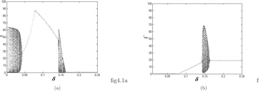
ω3 = 0.9, and ω4 = 0.12, model system (2.2) possesses different types of attractors as the parameter δ, the
total death rate of predator population is varied as shown in Fig. 3. The range of values of the parameters are chosen on the basis of the values reported in Jorgensen [34] and in the previous study by Upadhyay et al. [63], Roy and Upadhyay [54], Chattopadhyay et al. [11]. In-spite of the abundant literature on wild rabbit biology, knowledge on basic biological parameters from natural free populations is still lacking. However, numerical simulations are performed using ecologically permissible parameter values. For example, true conversion rates ofS andI toP are set to beω4/ω1= 0.24 andω3/ω2= 0.2, respectively, which are close to each other. Since,
both susceptible and infected rabbits are of the same kind, so these conversion rates must take close values. Alternatively,ω4/ω1> ω3/ω2, if predation of healthy rabbits leads to more reproduction than that of infected.
Also predation coefficients for S andI are set to be ω1= 0.5, ω2 = 4.5,which indicates that infected rabbits
are much frequently attacked by predators than susceptible rabbits. This is based on the fact that rabbits can be caught more easily due to their reduced ability to escape and hence ω2 must be larger thanω1. This set of