Searching for spectroscopic binaries within transition disk objects

SEARCHING FOR SPECTROSCOPIC BINARIES WITHIN TRANSITION DISK OBJECTS

Saul A. Kohn1,2, Evgenya L. Shkolnik1,3, Alycia J. Weinberger4, Joleen K. Carlberg5, and Joe Llama1,6

1

Lowell Observatory, 1400 W. Mars Hill Road, Flagstaff, AZ 86001, USA;[email protected]

2

Department of Physics and Astronomy, University of Pennsylvania, Philadelphia, PA, 19104, USA

3

School of Earth and Space Exploration, Arizona State University, Tempe, AZ 85287, USA

4

Department of Terrestrial Magnetism, Carnegie Institution of Washington, 5241 Broad Branch Road, NW, Washington, DC 20015, USA

5_{NASA/GSFC Code 667, Greenbelt, MD 20771, USA} 6

SUPA, School of Physics & Astronomy, North Haugh. St Andrews. Fife. KY16 9SS, UK

Received 2015 April 8; accepted 2016 January 28; published 2016 March 10

ABSTRACT

Transition disks (TDs) are intermediate stage circumstellar disks characterized by an inner gap within the disk structure. To test whether these gaps may have been formed by closely orbiting, previously undetected stellar companions, we collected high-resolution optical spectra of 31 TD objects to search for spectroscopic binaries

(SBs). Twenty-four of these objects are in Ophiuchus and seven are within the Coronet, Corona Australis, and Chameleon I star-forming regions. We measured radial velocities for multiple epochs, obtaining a median precision of 400 ms−1. We identified double-lined SB SSTc2d J163154.7–250324 in Ophiuchus, which we determined to be composed of a K7(±0.5)and a K9(±0.5)star, with orbital limits ofa<0.6 au andP<150 days. This results in an SB fraction of0.04-+0.030.12in Ophiuchus, which is consistent with other spectroscopic surveys of non-TD objects in the region. This similarity suggests that TDs are not preferentially sculpted by the presence of close binaries and that planet formation around close binaries may take place over similar timescales to that around single stars.

Key words:binaries: spectroscopic –circumstellar matter– stars: pre-main sequence

1. INTRODUCTION

Transition disks (TDs) are an intermediate stage of circumstellar disk evolution among pre-main sequence (PMS) stars. They are characterized by a lack of near-infrared excesses caused by inner optically thin holes or “gaps”opening within the disk structure, which typically have radii between one and tens of au and large far-infrared excesses from the disk material at larger separations(e.g., Hughes et al.2007,2009; Andrews et al.2011; Zhu et al.2011).

Planet formation and dust aggregation are thought to cause the gaps observed in TDs, with inner holes greater than 15 au possibly due to the formation of multiple planets ( Dodson-Robinson & Salyk2011; Zhu et al.2011). Other gap-formation mechanisms may involve ultraviolet (UV)and X-ray photons irradiating the disk and accretion from the disk onto the host star (e.g., Gorti et al. 2009; Espaillat et al. 2012). Recent observations by Follette et al. (2013) support the results of simulations from, e.g., Rice et al. (2006) and Zhu & Stone

(2014) that dust dynamics may play a role in gap formation. The distribution of large and small grains in the inner regions of disks can be modified by gas pressure gradients, perhaps also generated by planets, that may trap orfilter large grains as well as allow grains to grow efficiently(e.g., Zhu et al.2011; Pinilla et al. 2012).

A closely orbiting stellar companion may also produce an inner gap in a circumstellar disk(Artymowicz & Lubow1994; D’Alessio et al. 2005), as illustrated by the CoKu Tauri/4 system. This system was observed to have a 10 au wide gap

(Forrest et al.2004). The initial interpretation for such a wide gap was that a 10MJupplanet orbiting the central star cleared

out the material (Quillen et al. 2004). However, it was afterward shown that CoKu Tauri/4 was in fact a close visual binary (VB) system with a separation of ∼8 au (Ireland &

Kraus2008), and that the secondary star likely carved out the gap. Similarly, Biller et al.(2012)also detected a VB within the TD object HD 142527. With a projected separation of

(12.8±1.5 au), the companion is likely to have played a role in shaping the system’s complex disk structure, and it may have been responsible for the disk’s cleared inner ring.

A close binary system need not preclude circumbinary planet formation. Using photometric data from Kepler, Doyle et al.

(2011)announced thefirst discovery of a circumbinary planet. Several other circumbinary planets have since been discovered

(e.g., Orosz et al. 2012; Qian et al. 2012, 2012b; Schwamb et al.2013). These examples illustrate the need to further study multiple-star systems that host circumbinary material, and to test the effects of companion stars on disk dissipation and planet formation. Young star-forming regions(SFRs)are good test beds for such a study.

The nearby (140 pc) Ophiuchus star-forming region

(Oph)SFR contains a population of young stars of an average age ∼2.2 Myr (Wilking et al. 2005; Lombardi et al. 2008; Erickson et al. 2011). More than 50% of the young stellar objects (YSOs) in Oph show evidence of optically thick circumstellar disks at mid-IR wavelengths (Bontemps et al. 2001), of which 9% are identified as TDs (Evans et al. 2003; Cieza et al. 2010). This makes it well-suited for studies of disk dissipation.

Previous surveys of multiplicity in Oph and other SFRs have concentrated on visual binarity across all of the known active star-forming regions (e.g., Table6 of Lafreniere et al. 2008). With the exception of interferometric methods that are sensitive to separations of order 0.1–1 au(Pott et al.2010), VB searches are typically limited to separations <4 au (Ghez et al. 1993; Kraus et al.2012). Cieza et al.(2010) (hereafterC10)used IR and optical data to identify the TDs in Oph. C10 also sub-classify the TDs in their sample into five catagories: grain growth-dominated disks (which are accreting and have a negative slope of IR excess: 44% of their sample), giant planet-The Astrophysical Journal,_820:2(_15pp)_{, 2016 March 20 doi:10.3847}/_0004-637X/₈₂₀/₁/₂ © 2016. The American Astronomical Society. All rights reserved.

*_{This paper is based on data gathered with the 6.5 m Clay Telescope located at}

Las Campanas Observatory, Chile.

forming disks (accreting with a positive slope of IR excess: 13%), photoevaporating disks (non-accreting with high disk luminosity: 17%), disks already in the debris disk stage( non-accreting with low disk luminosity: 13%) and circumbinary disks (13%). C10 did not observe an increase in detected companions within the separations to which their survey was most sensitive (8–20 au) compared with other separations, leading them to suggest that stellar companions at these separations are not responsible for a large fraction of the TD population.

We present a complementary radial velocity(RV)survey to C10 to search for stellar companions closer in to the primary star. Our aim is to test whether the spectroscopic binary (SB) fraction is similar or enhanced in the TD population relative to stars without such disks. The structure of this paper is as follows. The selection of the TD systems, observations and data reduction are described in Section 2. RV, rotational velocity, and spectral type (SpT) measurements are presented in Section 3. We report the discovery of a double-lined spectroscopic binary in Section4 and evaluate possible biases and the completeness of our survey in Section 5. We derive a multiplicity fraction for Oph TDs, compare with previous multiplicity surveys of Oph, and discuss what multiplicity among TD objects might mean for theories of disk dispersal in Section6. We summarize and conclude our study in Section7. While not the main objective of this paper, we provide values of lithium I(LiI)and Hαequivalent widths(EWs), accretion

rates for our sample, and a discussion on the unusual nature of Oph star SR21A in the Appendix.

2. SAMPLE AND OBSERVATIONS

To survey the innermost regions of TD objects for stellar companions, we collected multi-epoch, high-resolution optical spectroscopy of 24 stars in Oph identified as having TDs(C10; Andrews & Williams 2007a; Geers et al. 2007; Furlan et al. 2009), two in Corona Australis (CrA;<3 Myr; Neuhauser & Forbrich2008; Sicilia-Aguilar et al.2008; Hughes et al.2010), two in Coronet (Cor, embedded within CrA;<1 Myr; Knacke et al.1973; Sicilia-Aguilar et al.2008; Hughes et al.2010), and

three in Chameleon I(Cha; 1–3 Myr; Furlan et al.2009; Kim et al.2009).

C10identified Oph TDs from their colors as measured by the

Spitzer Cores 2 Diskslegacy program(Evans et al.2003)and 20 of our 24 targets come from that work. A Spitzer color

(where[x]indicates the magnitude in thexμm band)of[3.6]– [4.5]<0.25 indicates theflux deficit characteristic of the near-infrared/inner opacity holes of a TD, while a color of [3.6]– [24]>1.5 ensures that all of the targets have significant mid-IR excesses at 24μm. We included an additional four Oph targets and seven from other regions, all of which were identified by other authors using the same criteria as C10

(Andrews & Williams 2007a; Geers et al. 2007; Furlan et al.2009).

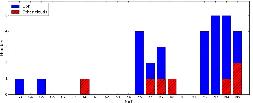
The Oph targets in this study are shown in Figure 1 in relation to other surveys of YSOs in the region. Table 1 lists each target in our sample, its stellar association, coordinates, SpT, and V, R, and J magnitudes. Targets that have known wide stellar companions are also noted. The SpT distribution of our sample is shown in Figure2and is dominated by late-K to mid-M stars with a median SpT of M2.

2.1. Observations

We acquired high-resolution optical spectra using the

Magellan Inamori Kyocera Echelle (MIKE; Bernstein et al. 2003) spectrograph at the Magellan (Clay) 6.5 m telescope. Twenty-one of our targets were observed twice, two or three days apart during 2010 June 18–23(UT100618– UT100623)7and then nearly a year later on 2011 June 14–15

(UT110614–UT110615). Two targets were observed a third time on 2012 May 9–10(UT120509–UT120510)and another on 2012 January 17 (UT120117). The complete log of our observations is recorded in Table2. We used the red arm of the spectrograph and the 0 5 slit to obtain a spectrum from 4900 to 9150Åwith a spectral resolution of∼47,000. Total exposure times ranged from 2 to 30 minutes per target depending on stellar brightness to achieve a typical signal-to-noise ratio

Figure 1.R.A. and decl.of our targets within Ophiuchus, overlaid with other multiplicity surveys. Contours are from theInfrared Astronomical Satellite(IRAS)Sky Survey Atlas at 100μm(Neugebauer et al.1984; Beichman et al.1988).

7

Table 1

Transition Disk Targets

Name Other Association α(J2000) δ(J2000) SpT V R J(2MASS) Known Visual Multiplicitya _Sourceb

Identifier h m s °′″ mag mag mag (Separation in″)

SZ Cha Cha 10 58 16.8 −77 17 17.1 K0 12.68 L 9.25 Binary(∼5) (1),(2),(3),(4)

T25 Sz 18 Cha 11 07 19.1 −76 03 04.8 M2.5 15.35 13.7 10.96 L (1),(5)

T35 Sz 27 Cha 11 08 39.0 −77 16 04.2 K8 L 15.82 11.17 L (1),(5)

RX J1852.3–3700 CrA 18 52 17.3 −37 00 12.0 K7 12.19 L 9.77 L (7),(8)

CrA-4111 CrA 19 01 20.8 −37 03 03.0 M4.5 L L 13.23 L (9)

G-49 CrA 468 Cor 19 01 49.4 −37 00 28.0 M4 L 16.6 12.5 L (9),(10)

G-102 CrA 133 Cor 19 01 25.6 −37 04 53.0 M5 L 15.3 12.36 L (9),(5)

SSTc2d J162118.5–225458 L Oph 16 21 18.5 −22 54 58.0 M2 L L 11.45 L (11)

SSTc2d J162218.5–232148 L Oph 16 22 18.5 −23 21 48.0 K5 12.67 L 9.52 L (11),(12)

SSTc2d J162245.4–243124 L Oph 16 22 45.4 −24 31 24.0 M3 L 14.2 10.38 L (11),(5)

SSTc2d J162309.2–241705 L Oph 16 23 09.3 −24 17 03.0 M? 12.75 14.2 10.32 L (1),(5)

SSTc2d J162332.8–225847 L Oph 16 23 32.8 −22 58 47.0 M5 15.7 11.49 L (11),(5)

SSTc2d J162336.1–240221 L Oph 16 23 36.1 −24 2 21.0 M5 14.68 L 11.53 L (11),(13)

SSTc2d J162506.9–235050 L Oph 16 25 06.9 −23 50 50.0 M3 L L 11.05 (11)

SSTc2d J162623.7–244314 DoAr 25 Oph 16 26 23.7 −24 43 14.0 K5 L 12.65 9.39 L (11),(14)

SSTc2d J162646.4–241160 L Oph 16 26 46.4 −24 11 60.0 G5 L 13.9 9.68 Binary(0.58) (11),(14),(15)

DoAr28 Haro 1–8 Oph 16 26 47.4 −23 14 52.2 K? 13.84 12.1 9.89 L (16),(17),(5)

SR21A L Oph 16 27 10.3 −24 19 12.7 G3 14.1 L 8.75 Binary(896) (18),(19),(20)

SSTc2d J162738.3–235732 DoAr 32 Oph 16 27 38.3 −23 57 32.0 K5 L 13.66 9.91 Triple(?)c (11),(14),(15),(21)

SSTc2d J162739.0–235818 DoAr 33 Oph 16 27 39.0 −23 58 18.0 K6 13.24 9.9 Triple(?)c _{(11),(14),(15),(21)}

SSTc2d J162740.3–242204 DoAr 34 Oph 16 27 40.3 −24 22 04.0 K5 11.5 11.1 8.44 L (11),(22)

SSTc2d J162802.6–235504 L Oph 16 28 02.6 −23 55 04.0 M3 L 11.76 L (11)

SSTc2d J162821.5–242155 L Oph 16 28 21.5 −24 21 55.0 M3 L 16.97 12.08 L (11),(14)

SSTc2d J162854.1–244744 L Oph 16 28 54.1 −24 47 44.0 M2 L 15.24 10.68 L (11),(14)

SSTc2d J163020.0–233108 L Oph 16 30 20.0 −23 31 08.0 M4 L L 11.32 L (11)

SSTc2d J163033.9–242806 L Oph 16 30 33.9 −24 28 06.0 M4 L L 11.63 L (11)

SSTc2d J163145.4–244307 L Oph 16 31 45.4 −24 43 07.0 M4 L L 11.8 L (11)

SSTc2d J163154.4–250349 L Oph 16 31 54.4 −25 03 49.0 M4 L L 11.78 L (11)

SSTc2d J163154.7–250324 Hα74 Oph 16 31 54.7 −25 03 24.0 K7 12.64 13.3 10.14 L (11),(5)

SSTc2d J163205.5–250236 L Oph 16 32 05.5 −25 02 36.0 M2 L 15.5 11.65 L (11),(5)

SSTc2d J163355.6–244205 L Oph 16 33 55.6 −24 42 05.0 K7 L 14.1 10.46 L (11),(5)

Notes.

a

Binary companions all lie outside of the TD. b

References:(1)Furlan et al.(2009);(2)Kim et al.(2009);(3)Ducati(2002);(4)Vogt et al.(2012);(5)Cutri et al.(2003));(6)Lopez Martí et al.(2013);(7)Hughes et al.(2010);(8)Kiraga(2012);(9)Sicilia-Aguilar et al.(2006);(10)Monet et al.(2003);(11)Cieza et al.(2010));(12)Vrba et al.(1993));(13)Allers et al.(2006);(14)Wilking et al.(2005);(15)Ratzka et al.(2005);(16)Andrews & Williams2007a);(17)Samus’et al.

(2003);(18)Geers et al.(2007);(19)Richichi & Percheron(2002);(20)Prato et al.(2003);(21)Barsony et al.(2005). The SpTs are from thefirst reference listed, followed by the references forVandRmagnitudes and then visual multiplicity, if applicable. AllJmagnitudes are from the 2MASS catalog(Skrutskie et al.2006).

c

SSTc2d J162738.3–235732 and SSTc2d J162739.0–235818 are both possible members of the same triple system about primary ROXs 30A(16h₂₇m_{37 0−23°59′32″; Ratzka et al.2005).}

3

The

Astrophysical

Journal,

820:2

(

15pp

)

,

2016

March

20

K

ohn

et

(S/N)of≈50 per resolution element at 8000Å. For the faintest stars, the S/N was roughly 10–20.

Data were reduced using the facility pipeline(Kelson2003). Each stellar exposure was bias-subtracted and flat-fielded for pixel-to-pixel sensitivity variations. After optimal extraction, spectra were wavelength calibrated with a ThAr arc taken within an hour of the stellar exposure. To correct for instrumental drift, the telluric molecular oxygen A band

(7619–7657Å) was used to align the MIKE spectra to an average precision of 70 ms−1. We then corrected for the heliocentric velocity.

3. RESULTS

3.1. Radial Velocities

Each target spectrum was cross-correlated against an RV standard star best matched to its SpT and observed on the same night. We used the IRAF8 fxcor routine (Wyatt 1985; Fitzpatrick 1993) to obtain RVs and search for single- and double-lined spectroscopic binaries (SB1s and SB2s, respec-tively). The standards and their published RVs are listed in Table3. We used orders 39, 40, 43, 44, 46, 48, 49, 51, and 53, which ranged from 6400 to 8900Å, for the cross-correlation to avoid telluric absorption lines and very low S/N regions. The RVs reported in Table2are the averages of those measured for each order weighted by the average S/N in each order. Table2 also lists the standard star used, and LiI and HαEWs (see

AppendixA.1for details of LiIand Hαanalysis).

The uncertainties in our RV measurements include the standard error on the mean RV across the cross-correlated apertures(typically∼400 ms−1), an uncertainty of 300 ms−1to account for RV distortions due to star spots on young stars

(Hatzes 2002; Mohanty et al.2002; Berdyugina2005; Desort et al.2007), and an additional 400 ms−1to account for the zero-point uncertainty in the RVs of our standard stars(see Table3), all added in quadrature. In all cases, the systematic uncertain-ties from possible spot activity and the zero-point dominate the final uncertainties. Note that Δ(RV), the difference in RVs

between epochs, need not include the uncertainty in the RV of the standards as the same standards were used.

The largest systematic uncertainties in these results will come from mismatched SpTs between the TD objects and the RV standard stars. While we endeavoured to match SpTs as closely as possible, the lack of G or K stars among our RV standards implies that for G and K-type TDs, systematics may remain unaccounted for. However, this should only affect SZ Cha(K0), SSTc2d SSTc2d J162646.4–241160(G5)and SR21A (G3–K?; a discussion of its SpT can be found in AppendixA.2), since late K-type stars can be well matched by early M-type standards. Indeed, we see that the uncertainties on the RVs of SZ Cha are larger(∼2×)than the average uncertainties.

The average RV of our Oph targets is−6.6 km s−1with a velocity dispersion of 1.3 km s−1, which agrees well with other measurements for the RV of the cloud: −5.64±2.57 km s−1 from Kurosawa et al. (2006) and −6.27±1.48 km s−1 from Prato (2007). There are no overlapping targets between our sample and those studies.

Our average RV for Cha targets is 15±1 km s−1, which is in good agreement with James et al. (2006), who report an average of 12.8±3.6 km s−1. However, our measurements of the average RV of CrA+Cor,−3±1 km s−1differs by∼1.5σ from James et al.ʼs findings of −1.1±0.5 km s−1. It is, however, in good agreement with Neuhäuser et al.(2000), who find an average RV of−2.6±1.4 km s−1forROSAT-selected T Tauri stars in CrA.

The close agreement in mean RV values within our sample implies that any single RV measurement that deviates by more than 3σ from the region average would be a highly probable RV-variable SB1(Kurosawa et al.2006; Prato2007). Wefind no such targets in our sample.

3.2. Rotational Velocities

We determined rotational velocities (vsini) following the

“Fourier Method”(e.g., Carroll1933; Gray1976,2005; Reiners et al.2001; Simón-Díaz & Herrero2007). Using telluric lines, we determined a small amount of instrumental broadening

(∼0.2Å), which we absorbed into model lines of zero rotation. We extracted the excess broadening due to rotation using the relatively high S/N LiI doublet at 6708Åand CaI at 6718Å.

While forbidden atomic transitions such as[FeIII]do not run the Figure 2.Spectral type distribution of the TD sample. All of the targets have ages„10 Myr.

8

Table 2

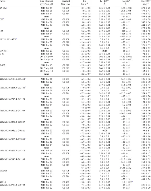
Observation Log and Measured Properties of TD Objects

Target Date observed Standard RV LiIEWa HαEWa Hα10%b

yyyy/mm/dd Star Used km s−1 _{Å Å km s}−1

SZ Chac _{2010 Jun 18 GJ 908 12.1±0.5 0.36±0.04 −3.68±0.03 270±25}

2010 Jun 21 GJ 908 14.0±1.5 0.38±0.02 −26.6±0.5 479±47 2011 Jun 14 GJ 514 17.0±1.3 0.42±0.05 −15.7±0.9 478±43

mean 14.0±2.0 0.39±0.07 −14±2 409±69

T25c 2010 Jun 18 GJ 908 15.3±0.3 0.55±0.02 −10.7±0.8 327±29

2010 Jun 21 GJ 908 15.6±0.3 0.58±0.02 −11±2 347±34 2011 Jun 14 GJ 514 16.0±0.3 0.60±0.04 −21±1 444±49

mean 15.7±0.6 0.58±0.05 −15±1 373±66

T35 2010 Jun 21 GJ 908 16.2±0.6 0.49±0.03 −118±15 482±45

2011 Jun 14 GJ 699 16.8±0.6 0.41±0.08 −128±16 520±55

mean 16.5±0.8 0.45±0.09 −123±22 501±71

RX J1852.3–3700d

2010 Jun 19 GJ 908 −1.5±0.3 0.5±0.1 −45±6 320±30 2010 Jun 22 GJ 699 −2.6±0.5 0.5±0.1 −33±2 325±33 2011 Jun 14 GJ 514 −3.0±0.3 0.48±0.01 −27±3 326±35

mean −2.4±0.6 0.5±0.2 −35±7 324±57

CrA-4111 2010 Jun 23 GJ 699 −5.2±0.3 <0.16 −16±4 135±14

G-49 2011 Jun 15 GJ 699 −2.7±0.3 0.51±0.04 −3±2 92±9

2012 May 09 GJ 699 −2.6±0.3 0.62±0.01 −4.32±0.05 106±10 2012 May 10 GJ 699 −2.8±0.3 0.62±0.01 −4.71±0.02 101±9

mean −2.7±0.6 0.55±0.09 −4±2 100±16

G-102 2011 Jun 15 GJ 699 −2.8±0.5 0.61±0.03 −14±4 189±18

2012 May 09 GJ 699 −2.9±0.3 0.66±0.01 −20±2 153±14 2012 May 10 GJ 699 −1.0±0.3 0.67±0.01 −17±1 152±7

mean −2.2±0.7 0.65±0.03 −17±4 165±24

SSTc2d J162118.5–225458c

2010 Jun 21 GJ 908 −6.3±0.4 0.48±0.01 −14.3±0.4 336±36 2010 Jun 22 GJ 908 −6.6±0.4 0.5±0.01 −8.9±0.7 285±30 mean −6.4±0.5 0.49±0.01 −11.6±0.8 310±47 SSTc2d J162218.5–232148c _{2010 Jun 19 GJ 908 −7.9±0.4 0.4±0.2 −8.2±0.2 362±40} 2010 Jun 21 GJ 908 −9.7±0.4 0.4±0.1 −15±1 551±53 2011 Jun 14 GJ 514 −7.5±0.4 0.42±0.03 −12.5±0.7 378±37

mean −8.4±0.7 0.4±0.2 −12±2 430±76

SSTc2d J162245.4–243124 2010 Jun 20 GJ 699 −5.3±0.3 0.5±0.4 −4.6±0.4 120±13 2010 Jun 22 GJ 699 −5.4±0.3 0.51±0.01 −5.1±0.8 124±12 2011 Jun 14 GJ 699 −4.0±0.3 0.55±0.05 −4.2±0.8 115±4

mean −4.8±0.6 0.5±0.4 −5±1 120±18

SSTc2d J162309.2–241705 2010 Jun 20 GJ 908 −3.8±0.4 0.28±0.06 −17.3±0.5 419±46 2010 Jun 22 GJ 908 −2.9±0.4 0.29±0.01 −16.3±0.8 365±30 2011 Jun 14 GJ 699 −3.6±0.4 0.29±0.01 −14±1 363±35

mean −3.4±0.7 0.29±0.06 −16±2 382±65

SSTc2d J162332.8–225847 2010 Jun 20 GJ 699 −6.9±0.3 0.54±0.01 −13±3 153±15 2010 Jun 22 GJ 699 −7.0±0.3 0.44±0.03 −11±3 122±13

mean −6.9±0.4 0.49±0.04 −12±4 137±20

SSTc2d J162336.1–240221 2010 Jun 20 GJ 699 −6.7±0.3 <0.28 −12±3 93±8

2010 Jun 22 GJ 699 −7.3±0.3 0.36±0.01 −8±1 113±11

mean −7.0±0.4 0.4±0.3 −10±3 103±14

SSTc2d J162506.9–235050c _{2010 Jun 20 GJ 699 −6.5±0.3 0.51±0.01 −9±1 259±26} 2010 Jun 22 GJ 699 −6.9±0.3 0.53±0.01 −12±3 341±34 2011 Jun 14 GJ 699 −7.0±0.3 0.57±0.01 −14±4 383±48

mean −6.8±0.6 0.53±0.01 −12±5 328±64

SSTc2d J162623.7–244314 2012 Jun 21 GJ 908 −7.2±0.4 0.5±0.2 −4.5±0.4 239±25 2011 Jun 14 GJ 908 −6.7±0.4 0.56±0.02 −11±1 467±47

mean −6.9±0.6 0.5±0.2 −8±1 353±53

SSTc2d J162646.4–241160 2010 Jun 20 GJ 908 −6.3±0.4 0.5±0.1 −11.7±0.4 346±31 2010 Jun 22 GJ 908 −6.6±0.3 0.4±0.2 −14.7±0.8 368±36 2011 Jun 14 GJ 514 −6.2±0.4 0.4±0.1 −17±2 356±34 mean −6.4±0.7 0.4±0.3 −14.38±2.2 357±58

DoAr28 2010 Jun 20 GJ 908 −8.6±0.3 0.45±0.01 −25±2 451±40

2010 Jun 22 GJ 908 −8.0±0.4 0.4±0.2 −29±2 441±47 2011 Jun 14 GJ 514 −7.9±0.3 0.4±0.2 −28±1 436±40

mean −8.2±0.6 0.4±0.3 −27±3 443±74

SR21A 2011 Jun 14 GJ 908 −3.6±0.5 0.13±0.02 1.1±0.15e L

SSTc2d J162738.3–235732 2010 Jun 19 GJ 908 −7.4±0.3 0.47±0.01 −16±2 291±33 2010 Jun 22 GJ 908 −6.5±0.3 0.49±0.02 −14±3 275±29

5

risk of confusing rotational broadening for thermal broadening, their S/N were consistently too low for use.

Our results were sensitive to the assumed limb-darkening coefficient,ò, with an∼15 km s−1deviation invsinifor a change

Δò∼0.1. Due to this sensitivity, we used the Claret(2000)linear limb-darkening coefficient catalog for each source, using characteristic values of logg and effective temperatures

(Gizis1997; Casagrande et al.2008; Rajpurohit et al.2013)for their literature SpTs(for G and K stars)and those determined by their TiO-7140 indices(for M stars; see Section3.3).

For each observation, we took a S/N-weighted average of the vsini as measured from the LiI and CaI lines. For each

target, we took the average of the per-observation measure-ments. Uncertainties were added in quadrature. Two targets in our sample havevsinimeasurements reported in the literature: RX J1852.3–3700 (23.05±3.59 km s−1 White et al. 2007); and SSTc2d J162740.3–242204 (14.7±0.9 km s−1 Torres et al. 2006). Both values are within the uncertainties of our measured values. We present our measurements in Table4.

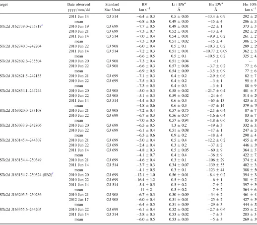
Table 2

(Continued)

Target Date observed Standard RV LiIEWa HαEWa Hα10%b

yyyy/mm/dd Star Used km s−1 _{Å Å km s}−1

2011 Jun 14 GJ 514 −6.4±0.3 0.5±0.05 −13.4±0.9 292±29

mean −6.8±0.6 0.49±0.05 −15±4 286±53

SSTc2d J162739.0–235818c

2010 Jun 19 GJ 699 −7.7±0.5 0.49±0.01 −22±1 373±37 2010 Jun 21 GJ 699 −7.3±0.7 0.52±0.01 −13±4 282±28 2011 Jun 14 GJ 514 −7.0±0.4 0.54±0.01 −9.9±0.2 261±27

mean −7.3±0.9 0.51±0.02 −15±4 306±54

SSTc2d J162740.3–242204 2010 Jun 22 GJ 908 −6.0±0.4 0.5±0.1 −10.3±0.2 289±29 2011 Jun 14 GJ 514 −7.2±0.3 0.51±0.01 −10.77±0.09 362±32

mean −6.6±0.5 0.5±0.1 −10.5±0.2 325±43

SSTc2d J162802.6–235504 2010 Jun 20 GJ 908 −7.3±0.4 0.51±0.04 <1 L

2010 Jun 22 GJ 908 −6.6±0.3 0.57±0.08 −3.7±0.2 77±6

mean −6.9±0.5 0.54±0.09 −3.5±0.9 77±6

SSTc2d J162821.5–242155 2010 Jun 21 GJ 699 −7.1±0.3 0.4±0.2 −2.9±0.6 82±7 2010 Jun 22 GJ 699 −7.5±0.3 0.4±0.2 −3±1 95±5

mean −7.3±0.5 0.4±0.3 −3±1 88±9

SSTc2d J162854.1–244744 2010 Jun 20 GJ 908 −5.0±0.3 0.58±0.02 −21.7±0.4 401±37 2010 Jun 22 GJ 908 −5.1±0.3 0.59±0.02 −24±6 314±29 2011 Jun 14 GJ 514 −4.4±0.3 0.6±0.3 −65±13 423±52

mean −4.8±0.6 0.6±0.3 −37±14 379±70

SSTc2d J163020.0–233108 2010 Jun 21 GJ 908 −7.2±0.4 0.57±0.75 −2.1±0.4 87±7 2010 Jun 22 GJ 699 −6.7±0.3 0.56±0.57 −1.6±0.4 83±7

mean −7.0±0.5 0.57±0.94 −1.8±0.6 85±10

SSTc2d J163033.9–242806 2010 Jun 20 GJ 699 −6.5±0.5 1.3±0.2 −19±3 332±33 2010 Jun 22 GJ 699 −6.1±0.4 0.51±0.08 −17±1 247±24

mean −6.3±0.6 0.9±0.2 −18±4 290±41

SSTc2d J163145.4–244307 2010 Jun 21 GJ 699 −5.0±0.4 0.5±0.4 −12.2±0.2 455±49 2010 Jun 22 GJ 699 −2.4±0.4 0.3±0.2 −37±2 446±39 2011 Jun 14 GJ 699 −4.8±0.3 0.5±0.05 −60±9 364±37

mean −4.1±0.7 0.4±0.4 −36±9 422±73

SSTc2d J163154.4–250349 2010 Jun 21 GJ 699 −4.6±0.4 0.3±0.1 −106±29 374±43 2011 Jun 14 GJ 514 −3.7±0.3 0.34±0.07 −139±33 402±35

mean −4.1±0.5 0.3±0.1 −123±44 388±56

SSTc2d J163154.7–250324(SB2)f 2010 Jun 20 GJ 699 −12.1±1.0 0.56±0.01 −8.4±0.2 394±38 2010 Jun 22 GJ 699 −16.4±1.2 0.5±0.2 −6±1 301±27 2011 Jun 14 GJ 514 −5.4±0.5 0.5±0.2 −7±2 397±39

mean −11±2 0.5±0.2 −7±2 364±61

SSTc2d J163205.5–250236 2010 Jun 21 GJ 908 −6.7±0.3 0.50±0.09 −34±2 461±43 2012 Jan 17 GJ 908 −6.0±0.4 0.51±0.01 −25±2 427±39

mean −6.4±0.5 0.51±0.09 −29±3 444±58

SSTc2d J163355.6–244205 2010 Jun 22 GJ 699 −6.1±0.4 0.52±0.02 −2.7±0.6 255±23 2011 Jun 14 GJ 514 −5.8±0.3 0.53±0.02 −7±3 283±31

mean −6.0±0.5 0.53±0.03 −5±3 269±39

Notes.

a

If the spectral line could not be distinguished from the continuum, a 2σlimit is shown.

b

Hα10% velocity width(White & Basri2003)variability is due to stellar activity or variable accretion(e.g., Jayawardhana et al.2003; Natta et al.2004).

c_{These targets were found to be active stars or variable accretors and are discussed in greater detail in AppendixA.1.} d

White et al.(2007)measured an RV of−1.46±2.21 km s−1_{, consistent with our measurements.}

e

Note that SR21A shows Hαin absorption rather than in emission. See AppendixA.2for further discussion of this object.

f

3.3. SpT Measurements

M-dwarf spectra are dominated by TiO molecular bands. Wilking et al. (2005)defined the TiO-7140 index as a way of determining the SpTs of M-dwarfs: a ratio of the meanflux of two 50Åbands centered on 7035Å(the continuum band)and

7140Å (the TiO band). We used the calibration given in Shkolnik et al.(2009)

=

-SpT (TiO 7140‐ 1.0911) 0.1755 ( )1

to measure the SpTs of all of our targets. Strictly, this relation holds for SpTs M0–M5, which covers the range of SpT literature values of M-dwarfs in our sample.9Our results are shown in Figure3. The error bars for literature values are±1 subclass, largely from C10. The error bars for our own measurements are the root mean square = 0.6 scatter of the Shkolnik et al.(2009)calibration, added in quadrature with the standard deviation of the measured SpTs across the multiple epochs each target was observed. They favor a linearfit of

=  + - 

SpTThis work (1.5 0.4 SpT) Lit. ( 2 1 ,) ( )2

i.e., we measure SpTs consistent with the literature values to ∼±1 SpT subclass. Our measured SpT per target is shown in Table 4 along with the literature values (see references in Table1)andvsini(see above). We do not revise K-type SpTs with the exception of SSTc2d J163154.7–250324, which we find to be an SB2(see Section4). For this system we report the derived SpTs andvsinifor each component. The lack of TiO in the spectra of the two G stars in our sample (SSTc2d J162646.4–241160 and SR21A)indicates that they are hotter than M stars, but the difference between very young G and K stars is not well-constrained (e.g., Beuther et al. 2014) and therefore we do not revise their SpTs.

4. SPECTROSCOPIC BINARY DETECTION

Single-lined SBs, SB1s are revealed by significant RV variability between observations. We performedχ2tests on the RVs of targets with single-peaked cross-correlation functions

Table 3 Radial Velocity Standards

Name Spectral Type RVa

km s−1

GJ 514 M1 14.56±0.40

GJ 699 M4 −110.51±0.40

GJ 908 M2 −71.15±0.40

Note.

a

RVs are taken from Nidever et al.(2002), who quote an RV stability of 0.05 km s−1_{. The zero point of the absolute RVs in this study is uncertain at the} 0.4 km s−1_{level(Marcy & Benitz1989).}

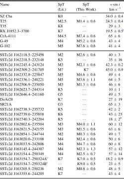
Table 4

Spectral Types and Rotational Velocities

Name SpT SpT vsini

(Lit.) (This Work) km s−1

SZ Cha K0 L 34.0±0.4

T25 M2.5 M1.4±0.6 24.3±0.4

T35 K8 L 29±3

RX J1852.3–3700 K7 L 19.5±0.5a

CrA-4111 M4.5 M7.4±0.6 65±6

G-49 M4 M5.2±0.6 43±4

G-102 M5 M7.6±0.6 41±4

SSTc2d J162118.5–225458 M2 M2.6±0.6 40±3

SSTc2d J162218.5–232148 K5 L 35±16

SSTc2d J162245.4–243124 M3 M2.1±0.6 42.3±0.2 SSTc2d J162309.2–241705 M? K? 45.0±0.9 SSTc2d J162332.8–225847 M5 M4.6±0.6 49±4 SSTc2d J162336.1–240221 M5 M3.6±1.1 64±5 SSTc2d J162506.9–235050 M3 M1.3±0.6 46±6

SSTc2d J162623.7–244314 K5 L 10±1

SSTc2d J162646.4–241160 G5 L 49±5

DoAr28 K? L 27±19

SR21A G3 L 65±3

SSTc2d J162738.3–235732 K5 L 42±2

SSTc2d J162739.0–235818 K6 L 43±23

SSTc2d J162740.3–242204 K5 L 18±2b SSTc2d J162802.6–235504 M3 M4.0±1.1 60±12 SSTc2d J162821.5–242155 M3 M1.5±0.6 63±6 SSTc2d J162854.1–244744 M2 M0.3±0.6 49±7 SSTc2d J163020.0–233108 M4 M2.4±0.6 50±6 SSTc2d J163033.9–242806 M4 M4.7±0.6 60±8 SSTc2d J163145.4–244307 M4 M2.3±1.3 57±12 SSTc2d J163154.4–250349 M4 M2.5±0.7 57±14 SSTc2d J163154.7–250324Ac K7 K7.0±0.5 18.2±0.9 SSTc2d J163154.7–250324Bc _L

K9.0±0.5 23±5 SSTc2d J163205.5–250236 M2 M0.8±0.6 48±5

SSTc2d J163355.6–244205 K7 L 43±4

Notes.

a

White et al.(2007)report avsini=23.05±3.59 km s−1 for this target, within 1σof our measured value.

b

Torres et al. (2006) report avsini=14.7±0.9 km s−1 for this target, within 2σof our measured value.

c_{This target is an SB2. In this Table we report the properties of each}

component. See Section4.

Figure 3.M-subclasses of targets reported as M-dwarfs in the literature(i.e., 

0 M0,1M1, etc.), with their literature subclasses compared with our own measurements based on their TiO-7140 indicies. A 1:1 relation is overlaid in blue. Our measurements are broadly consistent with the literature values. Larger deviations from the literature values at subclasses…5 occur because the TiO-7140 index is less well-constrained for late M SpTs.

9

An interesting case is that of the target SSTc2d J162309.2–241705, for which C10 report an uncertain SpT of “M?.” We measure a negative M-subclass for this target, suggesting that it may be a late K.

7

(CCFs)using the target’s average RV as aflat prior and found no SB1s in our sample of 31 TD objects. As mentioned above, the fact that all of the RVs agree with both the sample average for their SFR and the association average from the literature argues against any of our targets being long-period SB1s, or

P∼1 year systems whose RV was serendipitously measured by us at the same orbital phase each year.

Cross-correlation of the target spectra with an RV standard spectrum reveals whether a star is an SB2 if the orbital phase at the time of observation allows resolvable RV motion such that CCF is double-peaked. We found one SB2 in the sample

(SSTc2d J163154.7–250324), which we discuss in the subsections below.

4.1. Measured Properties of SSTc2d J163154.7–250324

The stellar features were blended enough on UT100620 and UT100622 that we could not confirm it as an SB2 using those observations alone. SSTc2d J163154.7–250324 clearly exhib-ited a double-peaked CCF one year later on UT110614. We measured the RVs of the primary and secondary components to be 16±2 km s−1 and −27±2 km s−1, respectively. This gives a systemic RV ofγ=−5.4±0.5 km s−1based onfluxes in the two CCF peaks (flux ratio of 0.68±0.07; see below). We measured values ofvsinifor the primary and secondary as 18.2±0.9 km s−1and 23±5 km s−1, respectively, following the method described in Section 3.2 on the unblended absorption lines seen on UT110614. A section of the stellar spectrum and the CCFs of this SB2 are shown in Figures4and 5 respectively.

Since we resolved the two CCF peaks, we were able to estimate SpTs and component masses of the individual stars. Assuming a flux-weighted relation (where fi is the integrated flux of Gaussianfits to the cross-correlation peaks at R band wavelengths; Figure 5) between component and integrated SpTs (Cruz & Reid 2002; Reid & Cruz 2002; Daemgen et al.2007)for primary starAand secondaryB:

= f +f f +f

SpTint ( ASpTA B SpTB) ( A B). ( )3

Using the Kepler’s Third law we related component masses

Mnto velocity amplitudesKn:

=

MA MB KA KB. ( )4

We imposed a limit on SpT and magnitude (Daemgen et al.2007; Shkolnik et al.2010):

D =R MR(SpTB)-MR(SpT .A) ( )5

We measure aflux ratio of 0.68±0.07 for the CCF peaks. Thus, we determine that SSTc2d J163154.7–250324 is composed of a K7(±0.5)and a K9(±0.5)star, with mass ratio

q;0.95. Using Kepler’s Third Law, we calculated the orbital limits to be a<0.6 au and period P<150 days. Our measurements of this system are summarized in Table5.

4.2. Comparison to the Literature

Before the SB2 SSTc2d J163154.7–250324 was identified as a TD, it had already been measured to have an infrared excess in its SED by 2MASS and exhibit the visible spectral properties of a YSO(Ratzka et al.2005, who refer to the system as Hα74 and/orISO-Oph 207). The disk is unresolved in the CHARM2 catalog(Richichi et al.2005). Padgett et al.(2008)reported the YSO to reside in the most populated region of the Oph SFR. Evans et al. (2009) reported J163154.7–250324 to have an extinction-corrected temperature and a luminosity of 3100 K and 2.5L_e, respectively. It is listed as a YSO candidate star with extinction from dust, but no evidence of local extinction

Figure 4. Spectrum of SSTc2d J163154.7–250324 on UT110614. The SB2 nature of the system is evident in all absorption features, including the Li lines at 6708Å.

Figure 5.CCFs of SSTc2d J163154.7–250324 averaged across apertures used. Spectra taken in 2010 were cross-correlated against GJ 699 and those in 2011 against GJ 514.

Table 5

Properties of the SSTc2d J163154.7–250324 System

Property System A B

SpT K7a _{K7.0±0.5 K9.0±0.5}

RV(km s−1_{) −5.4±0.5 16±2 −27±2}

vsini(km s−1_{) L 18.2±0.9 23±5}

Separation(au) <0.6 L L

Period(days) <150 L L

Mass ratio 0.95 L L

Note.

a

from a surrounding envelope. Cieza et al. (2009), like Ratzka et al.(2005), found no evidence for multiplicity.

C10identified the system as a TD and determined it to be a K7-type star, in agreement with our measurements above. Their LiI measurements were too low in S/N and therefore

unreported, so we cannot compare them to our own measure-ments of 0.5±0.2Å. They detected strong emission from the CaIItriplet, providing further evidence that it is indeed a PMS

object. Their measurement of the Hα 10% velocity-width

(470 km s−1) is similar to our own (364±61 km s−1), but variation is expected due to variable accretion and the SB2 nature of the object.C10found no evidence for a companion, as their study was not sensitive to separations <8 au. They derive a limit on disk mass ofMD<1.1MJupand classify it as

a grain growth-dominated TD(as mentioned in Section1, this is their most common TD subclass).

5. SAMPLE SENSITIVITY TO COMPANIONS

We proceeded in a completeness study of our results following Section6.1 of Duquennoy & Mayor (1991) and Section3.1 of Melo (2003), considering the observation cadence for each target, vsini, and the RV uncertainties of each spectrum. We sought to constrain how sensitive we were to SB1s within each TD for different orbital periods and secondary masses.

We estimated the primary mass of each target based on its absolute magnitude using low-mass solar metallicity stellar evolution models from Baraffe et al. (2015). To estimate absolute magnitudes we apply the distance to Oph of 140 pc, for Cha targets we used a distance of 160 pc (Feigelson & Lawson2004), and for CrA and Cor targets we use a distance of 140pc(Sicilia-Aguilar et al.2008). We use the Baraffe et al.

(2015) 1 Myr CFHT tracks for all targets (e.g., Furlan et al. 2009; Kim et al. 2009). The 2MASS J magnitudes, available for all of our targets(andKwhere available), coupled with these age and distance estimates allowed us to estimate the mass of each target. We did not correct for extinction; NIR magnitudes are the least affected by optical- and NIR-excesses from accretion and inner disks. The average change in mass estimate between the Baraffe et al. (1998) and Baraffe et al.

(2015)models was∣DM∣=0.2M_e. Such a difference has little impact on our results.

With these estimated primary masses of each target, we generated 106artificial companions, each with mass ratio(q), period(P), time of periastron, inclination(i), and longitude of periastron (ω) chosen randomly from a uniform distribution. Eccentricity (e) was chosen to be zero for P<8 days, and drawn from the Hyades distribution of Burki & Mayor(1986) for P>8 days. The solution of Kepler’s Equation followed Chapter 2.5 of Hilditch(2001). At each date of observation, we calculated the RV for each artificial companion and added to this a random uncertainty drawn from a Gaussian distribution centered around our measured uncertainty of the(real)primary RV(Table2).

To avoid an overestimate of detection probability at high mass ratios and long orbital periods (where we expect SB2 systems to lie in this (Msecondary,P)-space) we calculated the flux-weighted systemic velocity of the binary system

g= +

+

A A

A A

RV RV

6

1 1 2 2

1 2

( )

whereA2/A1is theflux ratio of the stars, and RV1and RV2are

the RVs of each star. Their orbits are related by angle

q2=q1+p, orbiting the center of mass. We interpolated the

fluxes in the I-band using the Baraffe et al.(2015)1 Myr CFHT tracks. Defining a1=cos(q1+w)+ecosw,

a2=cos(q1+p+w)+ecosw, and expressing the flux

ratio asFR=A2/A1, the systemic RV of the system is then

g= p a a

+ - +

a i

F P e M M F

2 sin

1 R 1 . 7

R

2 1 2 2 1 1 2

( ) ( ) ( ) ( )

We then tested if the artificial companion could be

“detected”by whether the root mean square of the values of

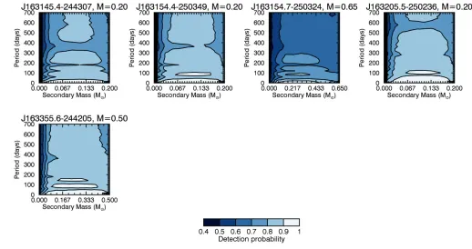
γ(each given by Equation(7))was greater than 0.7 km s−1, i.e., greater than the upper limit on the standard errors of our non-SB RVs. With over 106simulations per target, we were able to map probabilities of detection in (Msecondary,P)-space. The results of these simulations are shown in Figure6, which shows contour levels in 10% bins from 40% to 100% chance of detection.10 The periodic modulation in the contour patterns demonstrates our insensitivity to orbital periods that are multiples of our observing cadence.

The results of these simulations allow us to accurately assess our sensitivity to companions on a per-target basis, with a degeneracy inPand mass ratioq.11

For example, for SZ Cha we are sensitive to(…80% chance of detection)a 0.4M_ecompanion at periodsP<30 days and 70<P<75 days, whereas for SSTc2d J162623.7–244314 we are sensitive to a 0.4M_ecompanion at all periods. Such an example illustrates the challenge in quoting an “overall” or

“average” sensitivity for this non-homogeneous sample. We are, however, consistently sensitive to short-period(P<∼100 days)SBs for all of our targets.

6. DISCUSSION

Prato (2007) measures a spectroscopic binary fraction of

-+

0.12 0.04 0.08

among Oph K7-M4 stars. Of the 33 targets in Prato

(2007), two are TD objects but neither appears to be an SB: ROXR1 20(C10)and RX J1614.4–1857(Wahhaj et al.2010). Of the five SBs they found, one hosts a debris disk (RX J1612.6–1924, Wahhaj et al. 2010) and the rest are diskless

(RX J1612.3–1909, RX J1622.7–2325, and RX J1622.8–2333; Wahhaj et al. 2010; ROXR1 14 Cieza et al. 2007; Rosero et al. 2011). We found one SB2 in a sample of 24 Oph TD objects, and no SBs among the TD objects in the other SFRs surveyed. Including the two TD targets from Prato (2007) in our Oph sample, wefind that multiplicity among TD objects in this region to be 1/26. We measure an SB fraction of0.04-+0.030.12, determining uncertainties following the binomial theorem. This is consistent with that of the non-TD, late-type stars in Ophiuchus(Prato2007)and the young stars in Chameleon and Taurus–Auriga (0.07_-+_0.030.05 and 0.06_-+0.02

0.03_{, respectively; mass}

range 0.2–3M_e; Nguyen et al. 2009). The result is also in agreement with Lodieu et al.(2014), who report an SB fraction of 0.054±0.038 for wide binaries (50–150 au) in which one star is a planet-host. Their SB fraction for wide, planet-hosting substellar binaries is also within our range at 0.027±0.027.

10

While contour levels run between these values, they rarely go below a 60% chance of detection. This happens only for the lowest secondary masses.

11

One can convert between limits on the period and limits on the semi-major axis of separation a using the relation a P q M( , , primary)=

p +

P 2 2 3G 1 q M

primary1 3

( ) ( ( ) ) .

9

We also conclude that there is no significant difference between our result and that among the low-mass(0.08M_e–0.6M_e)field stars in the surveys of Duquennoy & Mayor(1991)and Fischer & Marcy (1992), 0.09_-+0.02

0.03 _and

-+

0.03 0.02

0.04_{, respectively.}

Like-wise, Raghavan et al. (2010) found an SB fraction of

-+

0.073 0.012

0.014 _{among nearby old solar-type dwarfs.}

That the fraction of SBs in TDs is similar to diskless stars

(within uncertainties) may suggest that whatever causes the disk dissipation is independent of binarity, i.e., disks around close SBs evolve on a similar timescale as those around single stars. Such a conclusion would mean that planet formation timescales around SBs may be comparable to those around single stars.

However, several studies (Ghez et al. 1997; White & Ghez 2001; Cieza et al. 2009; Duchêne 2010; Kraus et al.2012)have found protoplanetary disk fractions are lower for young („5 Myr) binary systems with a<50 au than for single stars or wider binaries. With the exception of Kraus et al.

(2012), these studies were not sensitive to the tight binary systems to which our study was especially sensitive. Kraus

et al.(2012) and Cheetham et al. (2015), sensitive to similar binary separations to our study, find the disk fraction among close visual binaries (0.1–40 au) in Taurus–Auriga and Ophiuchus to be lower than for single stars. Their studies did not distinguish between circumbinary TDs and other disk types

(e.g., debris disks). If the SB fraction of TD systems is actually lower than that in the diskless population, this suggests that the binary TD stage of a close-in binary is even shorter than the TD stage of single stars.

While we have searched for SBs specifically in TDs, Prato

(2007)made a complementary search for SBs irrespective of knowledge of their disks. None of the SBs she found were in transitional or protoplanetary disks. This is consistent with SBs having a faster TD phase and that the overall disk fraction among SBs remains low down to small separations.

Such a conclusion would be in contention with the results of Alexander (2012), whose models suggest that protoplanetary disks around tight binaries (a„1 au) are longer-lived than those around wider binaries. This is because the very close binaries efficiently clear the inner disk to radii larger the

Figure 6.Calculated contours in(Msecondary,P)-space representing the probability of detecting a companion star spectroscopically, given the precision and timing of

characteristic radius of photoevaporative winds, suppressing total disk dispersal.

That we onlyfind one SB in our TD sample could reflect that dissipation is so fast among these objects that most disks are completely dispersed by the age of Oph. However, we do not have the statistics to draw a steadfast conclusion. But since we find no evidence that TD objects have higher SB fractions than other stellar populations, we can infer that close-in binaries are not likely the primary cause of inner holes in TDs. This leads to giant planet formation as a more likely explanation.

7. SUMMARY

We have presented a spectroscopic survey of 31 TD stars, 24 of which lie in Ophiuchus. We found one of the Oph stars to be an SB2(SSTc2d J163154.7–250324). This system is composed of a K7(±0.5)and a K9(±0.5)star, with mass ratioq;0.95 and orbital limits a<0.6 au and P<150 days. The average RV of our Oph targets is −6.6 km s−1 with a dispersion of 1.3 km s−1. The median uncertainty in the measured RVs including systematic uncertainties is 0.4 km s−1. The average RVs of all four clouds surveyed(Cha, Cor, CrA and Oph)are consistent with the literature values. With this single SB detection, we measure an SB fraction of0.04_-+0.030.12. Thisfinding

is consistent with that of non-TD late-type stars in and outside of the region. This suggests that a TD may not be dispersed more efficiently by a tight binary than by a single star, and may imply that planet formation timescales around close binaries are comparable to those around single stars.

We thank M. Hughes for her contribution of RX J1852.3–3700 to the target list prior to its publication; L.Prato, C.Johns-Krull, and Cullen H.Blake for helpful discussions; and the anonymous referee for her/his insightful comments. S. A.Kohn acknowledges the support of NSF REU grant AST-1004107 through Northern Arizona University and Lowell Observatory. J. Llama acknowledges support from NASA Origins of the Solar System grant No. NNX13AH79G and from STFC grant ST/M001296/1. This research made use of the SIMBAD database, operated at CDS, Strasbourg, France.

Facility: LCO:Magellan(MIKE).

APPENDIX

We present here the accretion properties and Hαand LiI

measurements of individual stars.

Figure 6.(Continued.)

11

A.1. Age and Accretion Diagnostics

The strength of the LiI line (λ = 6708Å) is a standard

diagnostic for the age of low-mass stars, since lithium is rapidly depleted in their atmospheres. All but one of our targets exhibit LiIabsorption, so we are only able to place upper limits on the

absorption in the spectra of CrA-4111 due to low S/N in our single observation of the system. The LiI should be

undetectable in early M stars after ∼20 Myr (Baraffe et al. 1998; White & Hillenbrand 2005). For G and K stars the depletion can take much longer (…300 Myr, e.g., Zickgraf et al. 2005). The age of Oph is <10 Myr (Duncan 1981; Chabrier et al.1996; Martin et al.1999a,1999b; Zuckerman & Song2004,C10), and thus, all stars are expected to display Li absorption. For the 12 stars at sufficient S/N to detect Li that were also observed inC10, our EWs are consistent with theirs. Our LiI EW measurements of DoAr 28 and SR21A are

consistent with those of Magazzu et al.(1992)and James et al.

(2006), respectively. We are not aware of any previous measurements of LiI in SSTc2d J162309.2–241705. The LiI

EWs are listed in Table2.

Hα (λ=6563Å)is an indicator of stellar activity and gas accretion onto a star. Applying the relation found by Natta et al. (2004), we use the 10% velocity-width (White & Basri 2003) of the Hα emission to estimate the rate of accretion from the disk onto the star for targets with Hα10% velocity-widths greater than 200 kmbs−1(this is true for 21 of our 31 targets). We find that of the 15 targets that were observed byC10and had sufficient S/N at Hα, 10 have 10% velocity-widths within 3σ of those measured by C10. The large variations in the remaining measurements are likely due to variable accretion upon the star (e.g., Nguyen et al.2009). Six of our targets exhibited varying Hαduring our observa-tions as shown in Figure 7. These are SZ Cha, T25, SSTc2d J162118–225458, SSTc2d J162218–232148, SSTc2d

J162739–235818, and SSTc2d J162506–235050. The level of variability is unique for each target, but on average the EW varies by∼80%.

A.2. SR21A

At about 1–3 Myr old (which we note is older than the average age of Oph stars; Siess et al. 2000; Andrews et al. 2009; Brown et al.2009; Follette et al. 2013), SR21A is the primary component of a wide binary system in Oph (Barsony et al. 2005). Its SpT has been reported to be an early G(Suarez et al.2006; Andrews & Williams2007b), an early K (Struve & Rudkjobing 1949), and an M star

(Kimeswenger et al. 2004). Our measurements of its TiO-7140 index (see Section3.3)suggest it is not an M-type star

(SpTTiO<0). SR21A displays Hαin absorption rather than in emission,12the only such star in our sample. LiIabsorption is

also weaker than all of our other Oph objects. The Hαabsorption could be due to variable accretion(Johns-Krull & Valenti2001; Baraffe et al.2012; Hamilton et al.2012). This is suggested by the broadened blue shoulder of the absorption

(a feature possibly hidden by the NII absorption on the red

shoulder), a sign of possible accretion emission superimposing upon the photosphere absorption (Figure 8, left). Weak LiI

absorption(0.13±0.02Å; Figure 8, right)might suggest that SR21A is older than expected(<10 Myr; Chabrier et al.1996), but the existence of a TD is evidence against the star being >15 Myr(Mamajek2009; Muzerolle et al.2010). While James et al. (2006) find a slightly higher EW for LiI in SR21A (0.275±0.028Åversus our value of 0.13±0.02Å), they also note its inconsistency with other EWs in Oph. It is possible that the same episodic accretion that could be causing the

Figure 6.(Continued.)

12

Hαabsorption has also resulted in abnormal Li depletion in this star (Baraffe et al. 2009, 2012; Baraffe & Chabrier 2010). Depletion is also more realistic than the feature being veiled by accretion, since a disk hot enough for veiling would have caused SR21A to be disqualified as a TD object. However, we compared the EWs/line strengths of all of the lines in the same echelle order as the Li line in SR21A with the late K- and early M-type stars we observed on the same night(UT110614). We found that SR21A had weaker absorption for all lines,

suggesting that veiling may still play a role. Overall weaker lines might instead indicate a lower overall metallicity compared with the other Oph targets.

An extensive study of the disk morphology of SR21A was recently presented by Follette et al. (2013). Their results may support the postulate of a substellar companion present within the SR21A disk at∼18 au from the primary(Eisner et al.2009). Since we have just one observation of this system, we can neither confirm nor exclude thisfinding.

Figure 7.Variable accretion shown in Hα.

13

REFERENCES

Alexander, R. 2012,ApJL,757, L29

Allers, K. N., Kessler-Silacci, J. E., Cieza, L. A., & Jaffe, D. T. 2006,ApJ, 644, 364

Andrews, S., & Williams, J. 2007a,ApJ,671, 1800 Andrews, S. M., & Williams, J. P. 2007b,ApJ,671, 1800

Andrews, S. M., Wilner, D. J., Espaillat, C, et al. 2011,ApJ,732, 25pp Andrews, S. M., Wilner, D. J., Hughes, A. M., Qi, C., & Dullemond, C. P.

2009,ApJ,700, 1502

Artymowicz, & Lubow 1994,ApJ,421, 651 Baraffe, I., & Chabrier, G. 2010,A&A,521, A44

Baraffe, I., Chabrier, G., Allard, F., & Hauschildt, P. H. 1998, A&A, 337, 403

Baraffe, I., Chabrier, G., & Gallardo, J. 2009,ApJL,702, L27

Baraffe, I., Homeier, D., Allard, F., & Chabrier, G. 2015,A&A,577, A42 Baraffe, I., Vorobyov, E., & Chabrier, G. 2012,ApJ,756, 118

Barsony, M., Ressler, M. E., & Marsh, K. A. 2005,ApJ,630, 381

Beichman, C. A., Neugebauer, G., Habing, H. J., Clegg, P. E., & Chester, T. J.

(ed.)1988, Infrared Astronomical Satellite (IRAS)Catalogs and Atlases, Vol. 1(Washington, D. C.: NASA)

Berdyugina, S. V. 2005,LRSP,2, 8

Bernstein, R., Shectman, S. A., Gunnels, S. M., Mochnacki, S., & Athey, A. E. 2003, Proc. SPIE,4841, 1694

Beuther, H., Klessen, R., Dullemond, C., & Henning, T. 2014, Protostars and Planets VI(Tucson, AZ: Univ. Arizona Press)

Biller, B., Lacour, S., Juhász, A., et al. 2012,ApJL,753, L38 Bontemps, S., André, P., Kaas, A. A., et al. 2001,A&A,372, 173 Brown, J. M., Blake, G. A., Qi, C., et al. 2009,ApJ,704, 496

Burki, G., & Mayor, M. 1986, in IAU Symp. 118, Instrumentation and Research Programmes for Small Telescopes, ed. J. B. Hearnshaw, & P. L. Cottrell(Dordrecht: Riedel),385

Carroll, J. A. 1933,MNRAS,93, 478

Casagrande, L., Flynn, C., & Bessell, M. 2008,MNRAS,389, 585 Chabrier, G., Baraffe, I., & Plez, B. 1996,ApJL,459, L91

Cheetham, A. C., Kraus, A. L., Ireland, M. J., et al. 2015,ApJ,813, 83 Cieza, L., Padgett, D. L., Allen, L. E., et al. 2009,ApJL,696, L84 Cieza, L., Padgett, D. L., Stapelfeldt, K. R., et al. 2007,ApJ,667, 308 Cieza, L. A., Schreiber, M. R., Romero, G. A., et al. 2010,ApJ,712, 925 Claret, A. 2000, A&A,363, 1081

Cruz, K. L., & Reid, I. N. 2002,AJ,123, 2828

Cutri, R. M., Skrutskie, M. F., van Dyk, S., et al. 2003, 2MASS All Sky Catalog of Point Sources

Daemgen, S., Siegler, N., Reid, I. N., & Close, L. M. 2007,AJ,654, 558 D’Alessio, P., Merin, B., Calvet, N., Hartmann, L., & Montesinos, B. 2005,

RMxAA,41, 61

Desort, M., Lagrange, A.-M., Galland, F., Udry, S., & Mayor, M. 2007,A&A, 473, 983

Dodson-Robinson, S. E., & Salyk, C. 2011,ApJ,738, 131

Doyle, L. R., Carter, J. A., Fabrycky, D. C., et al. 2011,Sci,333, 1602 Ducati, J. R. 2002, yCat,2237, 0

Duchêne, G. 2010,ApJL,709, L114 Duncan, D. K. 1981,ApJ,248, 651

Duquennoy, A., & Mayor, M. 1991, A&A,248, 485

Eisner, J. A., Monnier, J. D., Tuthill, P., & Lacour, S. 2009,ApJL,698, L169 Erickson, K. L., Wilking, B. A., Meyer, M. R., Robinson, J. G., &

Stephenson, L. N. 2011,AJ,142, 140

Espaillat, C., Ingleby, L., Hernández, J., et al. 2012,ApJ,747, 103 Evans, N. J., II, Allen, L. E., Blake, G. A., et al. 2003,PASP,115, 965 Evans, N. J., II, Dunham, M. M., Jørgensen, J. K., et al. 2009,ApJS,181, 321 Feigelson, E. D., & Lawson, W. A. 2004,ApJ,614, 267

Fischer, D., & Marcy, G. 1992,ApJ,396, 178

Fitzpatrick, M. J. 1993, in ASP Conf. Ser. 52, Astronomical Data Analysis Software and Systems II, ed. R. J. Hanisch, R. J. V. Brissenden, & J. Barnes

(San Francisco, CA: ASP),472

Follette, K. B., Tamura, M., Hashimoto, J., et al. 2013,ApJ,767, 10 Forrest, W. J., Sargent, B., Furlan, E., et al. 2004,ApJS,154, 443 Furlan, E., Watson, D. M., McClure, M. K., et al. 2009,ApJ,703, 1964 Geers, V. C., van Dishoeck, E. F., Visser, R., et al. 2007,A&A,476, 279 Ghez, A. M., McCarthy, D. W., Patience, J. L., & Beck, T. L. 1997,ApJ,

481, 378

Ghez, A. M., Neugebauer, G., & Matthews, K. 1993,AJ,106, 2005 Gizis, J. E. 1997,AJ,113, 806

Gorti, U., Dullemond, C. P., & Hollenbach, D. 2009,ApJ,705, 1237 Gray, D. F. 1976, The Observation and Analysis of Stellar Photospheres(New

York: Wiley Interscience)

Gray, D. F. 2005, The Observation and Analysis of Stellar Photospheres

(Cambridge: Cambridge Univ. Press)

Hamilton, C. M., Johns-Krull, C. M., Mundt, R., Herbst, W., & Winn, J. N. 2012,ApJ,751, 147

Hatzes, A. 2002, AN,323, 392

Hilditch, R. W. 2001, An Introduction to Close Binary Stars (Cambridge: Cambridge Univ. Press)

Hughes, A. M., Andrews, S. M., Espaillat, C., et al. 2009,ApJ,698, 131 Hughes, A. M., Andrews, S. M., Wilner, D. J., et al. 2010,AJ,140, 887 Hughes, A. M., Wilner, D. J., Calvet, N., et al. 2007,ApJ,664, 536 Ireland, M. J., & Kraus, A. L. 2008,ApJL,678, L59

James, D. J., Melo, C., Santos, N. C., & Bouvier, J. 2006,A&A,446, 971 Jayawardhana, R., Mohanty, S., & Basri, G. 2003,ApJ,592, 282 Johns-Krull, C. M., & Valenti, J. A. 2001,ApJ,561, 1060 Kelson, D. 2003,PASP,115, 688

Kim, K. H., Watson, D. M., Manoj, P., et al. 2009,ApJ,700, 1017 Kimeswenger, S., Lederle, C., Richichi, A., et al. 2004,A&A,413, 1037 Kiraga, M. 2012, AcA,62, 67

Knacke, R. F., Strom, K. M., Strom, S. E., Young, E., & Kunkel, W. 1973,

ApJ,179, 847

Kraus, A. L., Ireland, M. J., Hillenbrand, L. A., & Martinache, F. 2012,ApJ, 745, 19

Kurosawa, R., Harries, T. J., & Littlefair, S. P. 2006,MNRAS,372, 1879 Lafreniere, D., Jayawardhana, R., Brandeker, A., Ahmic, M., &

van Kerkwijk, M. H. 2008,ApJ,683, 844

Lodieu, N., Pérez-Garrido, A., Béjar, V. J. S., et al. 2014,A&A,569, A120 Lombardi, M., Lada, C. J., & Alves, J. 2008,A&A,480, 785

Lopez Martí, B., Jimenez Esteban, F., Bayo, A., et al. 2013,A&A,551, A46 Magazzu, A., Rebolo, R., & Pavlenko, I. V. 1992,ApJ,392, 159

Mamajek, E. E. 2009, in AIP Con. Ser. 1158, ed. T. Usuda, M. Tamura, & M. Ishii(Melville, NY: AIP),3

Marcy, G. W., & Benitz, K. J. 1989,ApJ,344, 441

Martin, E. L., Basri, G., & Zapatero Osorio, M. R. 1999a,AJ,118, 1005 Martin, E. L., Delfosse, X., Basri, G., et al. 1999b,AJ,118, 2466 Melo, C. H. F. 2003,A&A,410, 269

Mohanty, S., Basri, G., Shu, F., Allard, F., & Chabrier, G. 2002,ApJ,571, 469 Monet, D. G., Levine, S. E., Canzian, B., et al. 2003,ApJ,125, 984 Muzerolle, J., Allen, L. E., Megeath, S. T., Hernández, J., & Gutermuth, R. A.

2010,ApJ,708, 1107

Natta, A., Testi, L., Muzerolle, J., et al. 2004,A&A,424, 603

Neugebauer, G., Habing, H. J., van Duinen, R., et al. 1984,ApJL,278, L1 Neuhauser, R., & Forbrich, J. 2008, in Handbook of Star Forming Regions, The

Southern Sky, Vol. II, Vol. 5, ed. B. Reipurth(San Francisco, CA: ASP),735 Neuhäuser, R., Walter, F. M., Covino, E., et al. 2000, A&AS,146, 323 Nguyen, D. C., Scholz, A., van Kerkwijk, M. H., Jayawardhana, R., &

Brandeker, A. 2009,ApJL,694, L153

Nidever, D. L., Marcy, G. W., Butler, R. P., Fischer, D. A., & Vogt, S. S. 2002,

ApJS,141, 503

Orosz, J. A., Welsh, W. F., Carter, J. A., et al. 2012,Sci,337, 1511 Padgett, D. L., Rebull, L. M., Stapelfeldt, K. R., et al. 2008,ApJ,672, 1013 Pinilla, P., Benisty, M., & Birnstiel, T. 2012,A&A,545, A81

Pott, J.-U., Perrin, M. D., Furlan, E., et al. 2010,ApJ,710, 265 Prato, L. 2007,ApJ,657, 338

Prato, L., Greene, T. P., & Simon, M. 2003,ApJ,584, 853 Qian, S.-B., Liu, L., Zhu, L.-Y., et al. 2012,MNRAS,422, 24 Qian, S.-B., Zhu, L.-Y., Dai, Z.-B., et al. 2012b,ApJL,745, L23

Quillen, A. C., Blackman, E. G., Frank, A,., & Varniere, P. 2004, ApJL, 612, L137

Raghavan, D., McAlister, H. A., Henry, T. J., et al. 2010,ApJS,190, 1 Rajpurohit, A. S., Reylé, C., Allard, F., et al. 2013,A&A,556, A15 Ratzka, T., Kohler, R., & Leinert, C. 2005,A&A,437, 611 Reid, I. N., & Cruz, K. L. 2002,AJ,123, 2806

Reiners, A., Schmitt, J. H. M. M., & Kürster, M. 2001,A&A,376, L13 Rice, W. K. M., Armitage, P. J., Wood, K., & Lodato, G. 2006, MNRAS,

373, 1619

Richichi, A., & Percheron, I. 2002,A&A,386, 492

Richichi, A., Percheron, I., & Khristoforova, M. 2005,A&A,431, 773 Rosero, V., Prato, L., Wasserman, L. H., & Rodgers, B. 2011,AJ,141, 13 Samus, N. N., Goranskii, V. P., Durlevich, O. V., et al. 2003, AstL,

29, 468

Schwamb, M. E., Orosz, J. A., Carter, J. A., et al. 2013,ApJ,768, 127 Shkolnik, E., Liu, M. C., & Reid, I. N. 2009,ApJ,699, 649

Shkolnik, E. L., Hebb, L., Liu, M. C., Reid, I. N., & Collier Cameron, A. 2010,

ApJ,716, 1522

Sicilia-Aguilar, A., Hartmann, L., Calvet, N., et al. 2006,ApJ,638, 897 Sicilia-Aguilar, A., Henning, T., Juhasz, A., et al. 2008,ApJ,687, 1145 Siess, L., Dufour, E., & Forestini, M. 2000, A&A,358, 593

Simón-Díaz, S., & Herrero, A. 2007,A&A,468, 1063

Skrutskie, M. F., Cutri, R. M., Stiening, R., et al. 2006,AJ,131, 1163 Struve, O., & Rudkjobing, M. 1949,ApJ,109, 92

Suarez, O., Garcia-Lario, P., Manchado, A., et al. 2006,A&A,458, 173 Torres, C. A. O., Quast, G. R., da Silva, L., et al. 2006,A&A,460, 695 Vogt, N., Schmidt, T. O. B., Neuhäuser, R., et al. 2012,A&A,546, A63 Vrba, F. J., Coyne, G. V., & Tapia, S. 1993,AJ,105, 1010

Wahhaj, Z., Cieza, L., Koerner, D. W., et al. 2010,ApJ,724, 835 White, R. J., & Basri, G. 2003,ApJ,582, 1109

White, R. J., Gabor, J. M., & Hillenbrand, L. A. 2007,AJ,133, 2524 White, R. J., & Ghez, A. M. 2001,ApJ,556, 265

White, R. J., & Hillenbrand, L. A. 2005,ApJL,621, L65

Wilking, B. A., Meyer, M. R., Robinson, J. G., & Greene, T. P. 2005,AJ, 130, 1733

Wyatt, W. F. 1985, in Stellar Radial Velocities, ed. A. G. D. Philip, & D. W. Latham(Schenectady: L Davis Press), 123

Zhu, Z., Nelson, R. P., Hartmann, L., Espaillat, C., & Calvet, N. 2011,ApJ, 729, 47

Zhu, Z., & Stone, J. M. 2014,ApJ,795, 53

Zickgraf, F.-J., Krautter, J., Reffert, S., et al. 2005,A&A,433, 151 Zuckerman, B., & Song, I. 2004,ARA&A,42, 685

15