Seismic Data Quality Control and Interpolation Using Principal Component Analysis

(1)

https://www.scirp.org/journal/ijg ISSN Online: 2156-8367

ISSN Print: 2156-8359

DOI: 10.4236/ijg.2019.1010054 Oct. 29, 2019 950 International Journal of Geosciences

Seismic Data Quality Control and Interpolation

Using Principal Component Analysis

Qingmou Li

1

_{, Sonya A. Dehler}

2

1_{Natural Resources Canada, Canadian Hazards Information Service (CHIS), Ottawa, ON, Canada} 2_{Natural Resources Canada, Geological Survey of Canada (Calgary), Calgary, Alberta, Canada}

Abstract

Commonly, seismic data processing procedures, such as stacking and pres-tack migration, require the ability to detect bad traces/shots and restore or replace them by interpolation, particularly when the seismic observations are noisy or there are malfunctioned components in the recording system. How-ever, currently available trace/shot interpolation methods in the spatial or Fourier domain must deal with requirements such as evenly sampled trac-es/shots, infinite bandwidth of the signals, and linear seismic events. In this paper, we present a novel method, termed the E-S (eigenspace seismic) me-thod, using principal component analysis (PCA) of the seismic signal to address the issue of reliable detection or interpolation of bad traces/shots. The E-S method assumes the existence of a correlation between the observed seismic entities, such as trace or shot gathers, making it possible to estimate one of these entities from all others for interpolation or seismic quality con-trol. It first transforms a trace (or shot) gather into an eigenspace using PCA. Then in the eigenspace, it treats every trace as a point with its loading scores of PCA as its coordinates. Simple linear, bilinear, or cubic spline 1 dimen-sional (1D) interpolation is used to determine PCA loading scores for any ar-bitrary coordinate in the eigenspace, which are then used to construct an in-terpolated trace for the desired position in physical space. This E-S method works with either regular or irregular sampling and, unlike various other published methods, it is well-suited for band-limited seismic records with curvilinear reflection events. We developed related algorithms and applied these to processed synthetic and offshore seismic survey data with or without simulated noises to demonstrate their performance. By comparing the inter-polated and observed seismic traces, we find that the E-S method can effec-tively assess the quality of the trace, and restore poor quality data by interpola-tion. The successful processing of synthetic and real data using the E-S me-thod presented in this approach will be widely applicable to seismic trace/shot interpolation and seismic quality control.

How to cite this paper: Li, Q.M. and Deh-ler, S.A. (2019) Seismic Data Quality Con-trol and Interpolation Using Principal Com-ponent Analysis. International Journal of Geosciences, 10, 950-966.

https://doi.org/10.4236/ijg.2019.1010054

Received: August 14, 2019 Accepted: October 26, 2019 Published: October 29, 2019

http://creativecommons.org/licenses/by/4.0/

(2)

DOI: 10.4236/ijg.2019.1010054 951 International Journal of Geosciences

Keywords

Seismic Quality Control, Seismic Interpolation, Eigenspace, Principal Component Analysis

1. Introduction

It is necessary to evaluate the quality of observed seismic records, and to detect and interpolate bad traces or shots [1][2], when the acquisition environment is challenging or when components of the sampling or recording system malfunc-tion. Seismic trace/shot interpolation is also critically required in multi-channel seismic data processing when the acquired data are coarser than the required spatial sampling as discussed in [3] [4]. However, many of the existing algo-rithms for data interpolation face challenges when dealing with seismic data having bad trace/shot data. For example, the local-slant-stack methods [5] are some of the oldest interpolation methods specifically developed for seismic data interpolation. To make these methods work effectively, algorithms must detect coherent events along with a set of dips in traces, and stack the data along the dip angle having the best semblance to create new reflectance. These methods have the very desirable feature of not requiring evenly spaced traces, as re-quired by many other methods. This means they can be used to interpolate aliased data and can handle irregularly recorded seismic data on complex land-scapes, such as in mountainous areas. However, these methods encounter chal-lenges in trying to identify complex reflection events and tend to have very large computing power requirements [3].

A significant advancement in seismic data interpolation came with the ap-pearance of the f-x method [6] and similar methods [7][8]. The idea behind these methods is to use the low-frequency components of the data to predict the high- frequency components by assuming that reflection events are linear in the tem-poral-spatial domain and that these events are aliased and unwrapped in the frequency domain. Clearly, the limitations of the f-x and related methods come from their linear events assumptions such that they are not suitable for curved events and practical band-limited seismic recording (aliased and unwrapped as-sumption). There are some extended versions of the f-x method, such as f-x-y method [6][9] [10], which works on areal (x-y) data in contrast to profile (x) data. However, they have the similar working principal and linear events assump-tions. Reference [11] proposes a minimum weighted norm method for curved seismic events but the method fails for aliased data.

(3)

DOI: 10.4236/ijg.2019.1010054 952 International Journal of Geosciences The 2 dimensional (2D) prediction error filter (PEF) as discussed in [13] works in temporal-spatial domain for predicting traces at half the trace interval of the seismic data. Reference [3] comments that the PEF method works in a manner that could be considered similar to f-x and f-k methods, although PEF works entirely in the time-spatial domain and has the limitations of being suitable only for linear events and infinite bandwidth records. Similar to the PEF method are the half-step [14] and multistep and autoregressively adapted pre-diction filter methods [8] [15] [16] for seismic interpolation. The multistep method further uses autoregression, or recursive least square solution, and adds a predefined exponential attenuation coefficient in the high-frequency compo-nents of prediction equations to relax the strict requirement of linear events as-sumption.

Reference [3] reviews, compares, and discusses some of these methods with their assumptions such as the requirement for linear events, infinite bandwidth records, and even special spatial sampling schemes. The linear assumption re-mains unresolved in the method of Fourier transformation for unevenly sampled records [17][18][19].

The method given by [20] predicts high frequency components from observed low frequency signals by solving the band-limited signal problem in the wavelet domain. Similarly, References [21][22] use curvelet and local radon transform to solve this prediction problem. However, the prediction of high frequency com-ponents from low frequency comcom-ponents is challenging without a solid physical foundation.

References [23][24][25][26][27] integrate migration and interpolation pro-cedures in wave equation-based imaging methods, such as reverse-time depth and Kirchhoff migration, for seismic interpolation in the Fourier or spatial do-mains. These methods have the advantage of noise attenuation while interpolat-ing seismic data. However, the migration method itself requires adequately in-terpolated seismic traces, and the issue of how to balance interpolation and mi-gration processes remains a challenge.

Reference [28] presents a nonlinear correlation technique to fill gaps in seis-mic surveys by replacing noisy traces using the correlation of adjacent traces. Unfortunately, it also assumes linear events (dip and amplitude) during the con-struction of synthetic (interpolated) traces.

Recently, References [29] [30] show promising results using artificial intelli-gence (AI), such as deep learning and convolution neural network, for seismic denoising and corrupted trace interpolation. However, it is difficult to under-stand why they succeed or fail because the coefficients of the trained network are not suitable for analysis.

Reference [31] released an inverse spatial PCA method for denoising and in-terpolating irregularly observed airborne magnetic survey data, with excellent results for separation of local anomalies during interpolation.

(4)

DOI: 10.4236/ijg.2019.1010054 953 International Journal of Geosciences for seismic data interpolation and quality evaluation, using PCA, without as-suming linear seismic events, infinite bandwidth, or regular spatial sampling. Currently, there is no published example showing this method and the appli-cations demonstrated in our study. Though many examples exist for seismic data processing using PCA [31]-[36], they are not applied to trace or shot in-terpolation and quality control. For example, Reference [34] focuses on de-noising by partial reconstruction of the seismic data image (array) using selected principal components (PCs) for vertical seismic profile data processing. Refer-ence [36] use a small fraction of PCs from PCA results of a stacking collection to replace this collection then feed this into the stacking procedure to get better stacking results. To enhance the computing efficiency, Reference [36] also pre-sents a fast PCA (FPCA) algorithm for practical seismic application. The 3 di-mensional (3D) seismic data reconstruction [32][34] is more similar to the pio-neering work made by [35] on using PCA for partial seismic data reconstruction, but they focused on fine-tuning of PCs and singular spectrum analysis (SSA) for energy structure, respectively. Reference [33] presents an abstract mentioning seismic trace interpolation using PCA but do not apply it to shot interpolation or seismic data quality control.

In the E-S method, we treat a seismic trace as a trace vector and arrange the trace vectors of any type of trace gather (e.g. common shot, common receiver, common mid-point, common offset, etc.) a trace matrix with its traces as rows, without losing any generality. For a shot gather, traces of a shot are concatenated to be a shot vector, after interpolation, we decipher the shot vector in the same way with the concatenation procedure. We fulfill the PCA of trace or shot matrix among their rows using the singular value decomposition (SVD) method to pre-serve energy and have high calculation performance.

In the following sections, we will first introduce the method and its data processing procedures (Section 2), and then test its performance using both a synthetic example and a trace and shot gather of offshore seismic data (Section 3). We discuss the working principal, possible improvement, and conclusions in Section 4.

2. The E-S Method

(5)

2.1. Constructing the Eigenspace

To simplify the descriptions, we will start from the E-S method using a common mid-point gather. Without losing any generality, we assume the seismic profile direction is x and acknowledge its m recorded traces with the trace sampling length (n). If we assume a trace at the line coordinate i (x = i) as a vector si (i

= 0, m − 1), then we can express this trace gather as an m * n matrix S:

(

)

T

0, , ,1 2 , m 1

s s s s ₋

=

S  (1)

where T means transpose of a matrix. All traces or rows of matrix S will span a vector-space [37] and all non-zero normalized principal components (PCs) of these traces (S) are created using PCA [38]. The PCs consist of an orthogonal base of the spanned eigenspace because of their unit length and mutually ortho-gonal properties. However, a better and more efficient way to construct the ei-genspace for eigenvector estimation and analysis of its energy structure is to de-compose the matrix S using the SVD method [39] as expressed in Equation (2), because the size of the seismic matrix S is often large

T =

S U VΣ (2) where S, U, ∑, and V are the seismic trace matrix, left eigenvector matrix, middle diagonal singular value matrix, and right eigenvector matrix with dimensions m * n, m * r, r * r, and r * n (r is the rank of matrix S), respectively. The columns of T

V are the bases of the constructed eigenspace and S has been mapped into the eigenspace having the rows of U as its loading scores or coordinates in the eigenspace, and the diagonal entries of ∑ as its spectrum reflecting its energy contribution. Note that rows and columns of U and T

V are unit (length) and mutually orthogonal, we can write any trace si as a row of S as:

(

)

(

)

T T

0, 1

i i i i i i i

s = Σu v =Σ u ×v i= m− (3)

where si, Σk, uk, ×, and

T

k

v are ith row of S, ithentry of ∑, ith row of U, outer

product, and ith_{column of} T

V , respectively.

2.2. Entity Interpolation in Eigenspace

Rows of matrix U are the coordinates of the entities, such as PCs of traces, in the eigenspace. According to Equation (3), seismic traces can be reconstructed in the eigenspace using T

V as its base and U as its “loading scores” (coordinates in the eigenspace) and its spectral density ∑ when the trace number i (i = 0, m − 1) or row of S is limited to be an integer. If we relax i to be a real number x (dis-tance along the seismic profile), such as 0.5 which means it locates in the middle between the first and second trace, then we can deduce the following equation from Equation (3):

( )

Σ T

x x i i

s = ×u v (4)

We define the constructed sx as a virtual trace at position x. During this pro-cedure, T

(6)

coor-DOI: 10.4236/ijg.2019.1010054 955 International Journal of Geosciences dinate trajectories of ui (Equation (3)) using a 1D interpolation method.

Prac-tically, we use the simple linear, bilinear or cubic spline 1D interpolation method to estimate ux (0.0≤ ≤x m) from U. Currently, we do not use the E-S method

for extrapolation outside the range of traces.

2.3. Bad Entity Detection

We can revise the E-S method for detection and restoration of bad traces if we compare any observed trace with its reconstructed trace from any other observa-tions using the E-S method. We use the residual mean square (rms) to evaluate the difference between the observed and reconstructed trace:

(

) (

)

T

1 i i i i i

S S S S

rms

n

′ ′

− ⋅ −

=

− (5)

where Si′ is the reconstructed trace at current trace location i (x = i) from the

trace gather not including the ith_trace.

Therefore, we start to detect bad traces from looping through all, except the first and last, traces in a trace gather by interpolating a new trace at the current looping trace location from the whole trace gather excluding the current one. Then we calculate and plot the rms of the observed and interpolated virtual ones. By examining the rms chart, we mark traces with rms bigger than our expected rms value, estimated from visual inspection of the rms chart, as bad traces and we replace them with the interpolated ones. To process noisy records with many bad traces, we repeat this procedure iteratively and pick only one trace as a bad trace in each iteration.

3. Numerical Tests

We test the E-S method with a simulated trace gather by convolving a synthetic reflectance coefficient profile, representing an unconformity and rift basin hori-zons, with a predefined Ricker wavelet that has frequency characteristics com-monly used in offshore seismic surveys. We also test the E-S method on a stacked trace gather from an offshore seismic survey that has horizons with steep dip, curved, onlap, offlap, and chaotic reflection of basin floor fans.

3.1. Synthetic Reflection Interpolation

To simulate a synthetic seismic profile, we draw a simulated stratigraphic profile with horizontal and curved interfaces and assign a constant reflectance to these horizons. Then we convolve this reflection trace gather with a predefined Ricker wavelet having 0.064 s duration, 100 Hz center frequency, and 2 ms sampling interval. We display the final simulated profile of 0.4 s and 100 traces in Figure 1(a) and its sparse traces (by extracting one from every two but keep the first and last traces) in Figure 1(b).

(7)

[image:7.595.62.537.73.436.2]

Figure 1. Interpolation of synthetic reflection section. (a) models seismic profile; (b) half traces of seismic models; (c) E-S results; (d) E-S residual.

we find the residual is close to zero and the E-S method has performed very well in the interpolation

3.2. Trace Interpolation

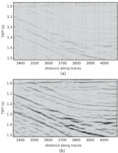
Next, we test the E-S interpolation method using a section of offshore seismic survey from the east coast of Canada, with 4 ms sampling interval, and show the results in Figures 2-8.

Figures 2-4 display the input traces (a), interpolation results (b), residuals (c), and rms (d) for interpolation using every second, third and fourth trace, respec-tively. Table 1 lists the mean errors and relative rms of trace interpolation using half of the original traces as shown Figure 2(d). The relative rms for others (Figure 3(d), Figure 4(d)) are all less than 30.0% of the standard deviation of the signal.

(8)

[image:8.595.260.482.69.346.2]

Figure 2. Trace interpolation using 1/2 of the original traces. (a) 1/2 Traces input; (b) E-S interpolated; (c) residual traces; (d) rms.

[image:8.595.264.479.390.692.2]

(9)

[image:9.595.262.477.69.380.2]

Figure 4. Trace interpolation using 1/4 of the original traces. (a) 1/4 Traces input; (b) E-S interpolated; (c) residual traces; (d) rms.

[image:9.595.214.534.429.692.2]

(10)

[image:10.595.255.493.63.299.2]

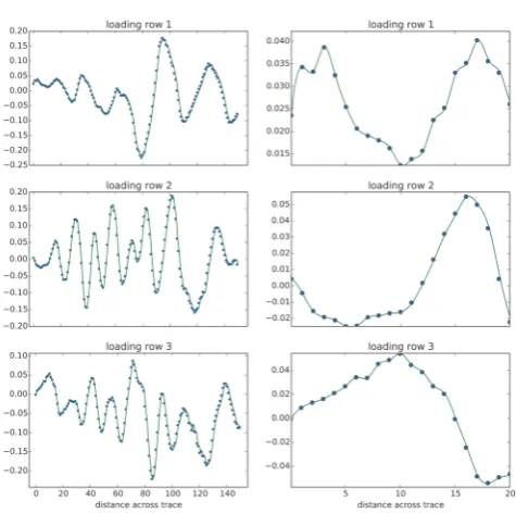
Figure 6. Examples of coordinates of known traces and their 1D interpolation in the ei-genspace. The dots (U) are known coordinates of the input traces in the eigenspace and solid lines are interpolated coordinates from these dots. The right column zooms to first twenty dots of corresponding coordinates of their left counterparts.

[image:10.595.127.538.369.712.2]

(11)

[image:11.595.268.475.69.338.2]

[image:11.595.209.540.439.486.2]

Figure 8. Five times expansion of the input traces by interpolation. (151 * 5 − 5 + 1) 751 traces are interpolated from the test 151 traces where every trace is 5 times interpolated between and including itself and next trace except the last trace where no extrapolation is made to avoid edge effects. (a) Input traces; (b) E-S interpolated traces.

Table 1. Calculated residual mean and rms values between original and interpolated traces using the E-S method.

Trace# ₃₃₆₉ ₃₃₈₉ ₃₄₀₉ ₃₄₂₉ ₃₄₄₉ ₃₄₆₉ _{3479 All traces}

Mean of errors −4.8 −2.3 3.0 7.4 −8 5.2 −1.4 2.4

rms 12.1% 12.9% 14.4% 16.3% 14.2% 18.9% 13.1% 100%

eigenbases, 90.3% on the first 31, and 99.1% for the first 60. The stronger the correlation that exists among traces, the faster the energy for every eigenbase (thin solid line in Figure 5) will attenuate, and simultaneously the faster the ac-cumulated energy will increase (dashed line in Figure 5). For white noise, the energy for every eigenbase is flat and there is no interpolation method that works under this circumstance.

We plot the spatial loading scores (and 1D interpolation trajectories) and ei-genbase in Figure 6 and Figure 7 to help to constrain the E-S method. In Figure 6, we display the coordinates (rows of U) with solid dots and its 1D interpolation with solid lines. We find these coordinates are quite smooth and suitable to be interpolated using simple 1D spline interpolation methods. We also show their local details in the right column of Figure 6 where the local smooth features are clear.

(12)

DOI: 10.4236/ijg.2019.1010054 961 International Journal of Geosciences may be useful in eigenspace base understanding.

In Figure 8, we use E-S interpolation to produce 5 times the initial number of traces to illustrate the resolution power in identifying basin floor fans, onlap, of-flap, and other structures of a rifted basin. In the input traces (Figure 8(a)), these sedimentary features of the rift basin are fuzzy and discontinuous. Howev-er, the rift basin structure is very clear in the interpolated section (Figure 8(b)), showing how the E-S method can be helpful in interpreting complex strati-graphic structures.

3.3. Bad Trace Detection

To test the performance of the E-S method for bad trace detection, we add nor-mal distribution noise n

(

µ σ,

)

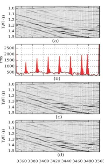
, as shown in Figure 9(a), to some randomly se-lected traces, such as [3369, 3389, 3409, 3429, 3449, 3469, 3479] in a trace gather (collection), using Equation (6), and we display the trace gather with simulated bad traces in Figure 9(c).

(

)

2.333 ,

noise

[image:12.595.288.458.327.595.2]

s = +s ∗n µ σ (6)

(13)

DOI: 10.4236/ijg.2019.1010054 962 International Journal of Geosciences where s and snoise are the original seismic trace, and the seismic trace with

added noise. The normal noise n has mean µ and standard deviation

σ

. We estimate µ and

σ

from the same trace where we add noise and 2.333 is a constant to control the signal to noise ratio.

We interpolate traces at any trace position, except the first and last, using the trace gather with added noises excluding current trace. Then we calculate the rms for each interpolated trace and display it as shown in Figure 9(b). From Figure 9(b), we can easily pick out bad traces and use the interpolated ones to fill corresponding traces to get Figure 9(d) for further processing or interpreta-tion without bad traces.

3.4. Bad Shots Detection and Interpolation

[image:13.595.122.535.416.680.2]

We use 120 shots from a seismic survey offshore east coast of Canada to test the performance of the E-S method for bad shot detection and shot interpolation. Every shot has 16 traces (receivers) and each trace has 1751 samples with 2 ms recording rate. The procedure is similar to the above example, in that noise was added to some shots, interpolation was used to produce a virtual shot using oth-er shots at evoth-ery shot location, and rms was calculated and plotted to detect bad shots. We display the rms chart example of these operations in Figure 10. The peaks of the rms chart as shown in Figure 10 correspond very well to the shot numbers where we added noise. We omit the display of shot gather for it is too large.

(14)

4. Discussion and Conclusions

In this paper, we propose a novel method termed Eigenspace Seismic (E-S) me-thod to improve seismic data quality and restore bad recordings, using PCA to interpolate in eigenspace.

We demonstrate the effectiveness of the E-S method for trace interpolation by processing synthetic and offshore seismic survey data to restore original data from decimated data sets with 1/2, 1/3, and 1/4 of the original traces. We also show its possible usage to clarify stratigraphic structures such as onlapping units and basin floor fans, in the interpolated trace gather by augmenting the number of original traces by a factor of 5 using the E-S method. The method works best for sparsely recorded or densely recorded seismic data with many bad compo-nents.

By analyzing the features of the E-S method using SSA, we can evaluate its energy distribution, features of eigenbases and the smoothness of loading scores (or coordinates in the eigenspace) trajectories that are helpful in the success of E-S method. The major advantage of the E-S method comes from the fact that it handles a whole trace or shot as an inseparable entity and transforms the 2D in-terpolation into a 1D problem in the eigenspace.

The computational cost of the E-S method is not an issue for trace interpola-tion and trace quality control, but it does become an issue for shot-gather inter-polation and quality control. The state-of-art fast PCA method [36] could be used to seamlessly speed up the E-S method.

The E-S method does not assume the signal is stationary so that it may be ef-fective for nonstationary noises commonly associated with marine data acquisi-tion, such as shark strikes, swell noise, or nonlaminar flow around cable instru-mentation. Theoretically, the E-S method is based on coherency of a processed trace so that it will be efficient to process seismic data having coherent signals. The effectiveness of the E-S method depends on the distribution of these noises on the PCs. There are some methods specifically designed to solve the energy concentration problems, such as factor analysis [38], that have possibility to ad-dress these requirements. These methods show great potential to improve the E-S method but their development is out of the range of this study.

Currently, we use simple 1D spline interpolation methods in the spatial load-ing score (U) interpolation in the E-S method. In the future, it should be possi-ble to use other advanced 1D interpolation methods for the U estimation to get better E-S results. There are many potential applications of the E-S method to seismic data or other datasets, such as the construction of a 3D velocity volume from irregularly distributed 3D velocity observations [40].

Acknowledgements

(15)

Geos-DOI: 10.4236/ijg.2019.1010054 964 International Journal of Geosciences cience Program partially supported this work. The authors wish to thank Mary- Lynn Dickson at the Geological Survey of Canada (Atlantic) for helpful discus-sions, Patrick Potter for preparing the offshore marine seismic reflection data and for constructive discussion, and John Shimeld for his critical internal review and suggestions. We also thank the Editors and two anonymous reviewers of the journal for their helpful suggestions for the improvement of the manuscript.

Conflicts of Interest

The authors declare no conflicts of interest regarding the publication of this pa-per.

References

[1] Yilmaz, O. (2001) Seismic Data Analysis: Processing, Inversion, and Interpretation of Seismic Data. Society of Exploration Geophysicists, Tulsa, OK, 1028 p.

https://doi.org/10.1190/1.9781560801580

[2] Sun, R. and Wang, A. (1998) Removing Bad Traces in Shallow Seismic Exploration. Tao, 9, 183-196. https://doi.org/10.3319/TAO.1998.9.2.183(T)

[3] Abma, R. and Kabir, N. (2005) Comparison of Interpolation Algorithms. The Leading Edge, 24, 984-989. https://doi.org/10.1190/1.2112371

[4] Fomel, S. (2003) Seismic Reflection Data Interpolation with Differential Offset and Shot Continuation. Geophysics, 68, 733-744. https://doi.org/10.1190/1.1567243

[5] Bardan, V. (1987) Trace Interpolation in Seismic Data Processing. Geophysical Pros-pecting, 35, 343-358. https://doi.org/10.1111/j.1365-2478.1987.tb00822.x

[6] Spitz, S. (1991) Seismic Trace Interpolation in the f-x Domain. Geophysics, 56, 785-796. https://doi.org/10.1190/1.1443096

[7] Gulunay, N. (2003) Seismic Trace Interpolation in the Fourier Transform Domain. Geophysics, 68, 355-369. https://doi.org/10.1190/1.1543221

[8] Naghizadeh, M. and Sacchi, D.M. (2009) f-x Adaptive Seismic-Trace Interpolation. Geophysics, 74, 9-16. https://doi.org/10.1190/1.3008547

[9] Spitz, S. (1990) 3-D Seismic Interpolation in the f-x-y Domain. SEG Technical Pro-gram Expanded Abstracts, 1641-1643. https://doi.org/10.1190/1.1890083

[10] Wang Y. (2002) Seismic Trace Interpolation in the f-x-y Domain. Geophysics, 67, 1232-1239. https://doi.org/10.1190/1.1500385

[11] Liu, B. and Sacchi, D.M. (2004) Minimum Weighted Norm Interpolation of Seismic Records. Geophysics, 69, 1560-1568. https://doi.org/10.1190/1.1836829

[12] Gulunay, N. and Chambers, R.E. (1996) Unaliased f-k Domain Trace Interpolation (UFKI). Society of Exploration Geophysicists, 1461-1464.

https://doi.org/10.1190/1.1826390

[13] Claerbout, J. (1998) Multidimensional Recursive Filters via a Helix. Geophysics, 63, 1532-1541. https://doi.org/10.1190/1.1444449

[14] Porsani, M. (1999) Seismic Trace Interpolation Using Half-Step Prediction Filters. Geophysics, 64, 1461-1467. https://doi.org/10.1190/1.1444650

[15] Naghizadeh, M. and Sacchi, D.M. (2007) Multistep Autoregressive Reconstruction of Seismic Records. Geophysics, 72, 111-118. https://doi.org/10.1190/1.2771685

(16)

DOI: 10.4236/ijg.2019.1010054 965 International Journal of Geosciences Generalized Fourier Transform. Geophysics, 76, 1-10.

https://doi.org/10.1190/1.3511525

[17] Duijndam, A.J.W., Schonewille, M.A. and Hindriks, C.O. (1999) Reconstruction of Band-Limited Signals, Irregularly Sampled along One Spatial Direction. Geophysics, 64, 524-538. https://doi.org/10.1190/1.1444559

[18] Zwartjes, P.M. and Sacchi, M. (2007) Fourier Reconstruction of Nonuniformly Sampled, Aliased Seismic Data. Geophysics, 72, 21-32.

https://doi.org/10.1190/1.2399442

[19] Guo, Z. (2017) Seismic Data Interpolation: The Arbitrary Sampled Fourier Trans-form Method. Master’s Dissertation, University of Calgary, Calgary, 66.

[20] Yu, Z., Ferguson, J., Mcmechan, G. and Anno, P. (2007) Wavelet-Radon Domain Dealiasing and Interpolation of Seismic Data. Geophysics, 72, 41-49.

https://doi.org/10.1190/1.2422797

[21] Wang, J.M. and Pert, M. (2010) Seismic Data Interpolation by Greedy Local Radon Transform. Geophysics, 75, WB225-WB234. https://doi.org/10.1190/1.3484195

[22] Herrmann, F.J. and Hennenfent, G. (2008) Non-Parametric Seismic Data Recovery with Curvelet Frames. Geophysical Journal International, 173, 233-248.

https://doi.org/10.1111/j.1365-246X.2007.03698.x

[23] Chen, H.W. and Chang, C.W. (1999) Implicit Noise Reduction and Trace Interpo-lation in the Wavefield Depth ExtrapoInterpo-lation. Geophysical Research Letters, 26, 3705-3708. https://doi.org/10.1029/1999GL005421

[24] Fu, L. (2004) Wave Field Interpolation in the Fourier Wave Field Extrapolation. Geophysics, 69, 257-264. https://doi.org/10.1190/1.1649393

[25] Oropeza, V. and Sacchi, M. (2011) Simultaneous Seismic Data Denoising and Re-construction via Multichannel Singular Spectrum Analysis. Geophysics, 76, 25

https://doi.org/10.1190/1.3552706

[26] Ronen, J. (1987) Wave-Equation Trace Interpolation. Geophysics, 52, 973-984.

https://doi.org/10.1190/1.1442366

[27] Trad, D. (2003) Interpolation and Multiple Attenuation with Migration Operators. Geophysics, 68, 2043-2054. https://doi.org/10.1190/1.1635058

[28] Martingson, D. and Hopper, J. (1992) Nonlinear Seismic Trace Interpolation. Geo-physics, 57, 136-145. https://doi.org/10.1190/1.1443177

[29] Mandelli, S., Lipari, V., Bestagini, P. and Tubaro, S. (2019) Interpolation and De-noising of Seismic Data Using Convolutional Neural Networks. arXiv:1901.07927v1. [30] Mikhailiuk, A. and Faul, A. (2018) Deep Learning Applied to Seismic Data

Interpo-lation. 80th EAGE Conference and Exhibition 2018, Extended Abstract.

https://doi.org/10.3997/2214-4609.201800918

[31] Li, Q. and Dehler, S.A. (2015) Inverse Principal Component Analysis for Geophysi-cal Survey Data Interpolation. Journal of Applied Geophysics, 115, 79-91.

https://doi.org/10.1016/j.jappgeo.2015.02.010

[32] Huang, W., Wang, R., Zhou, Y., Chen, Y. and Yang, R. (2016) Improved Principal Component Analysis for 3D Seismic Data Simultaneous Reconstruction and De-noising. SEG Technical Program Expanded Abstracts, 4102-4106.

https://doi.org/10.1190/segam2016-13858769.1

[33] Li, Q. and Dehler, S.A. (2012) E-x Method for Seismic Trace Interpolation, EGU General Assembly, Vienna, 22-27 April 2012, 6129.

(17)

Sec-DOI: 10.4236/ijg.2019.1010054 966 International Journal of Geosciences tions. SEG Technical Program Expanded Abstracts, 1261-1265.

https://doi.org/10.1190/1.1892508

[35] Wang, B. and Lu, W. (2017) Accurate and Efficient Seismic Data Interpolation in the Principal Frequency Wavenumber Domain. Journal of Geophysics and Engi-neering, 14, 1475-1488.https://doi.org/10.1088/1742-2140/aa82dc

[36] Wu, J. and Bai, M., (2018) Fast Principal Component Analysis for Stacking Seismic Data. Journal of Geophysics and Engineering, 15, 295-306.

https://doi.org/10.1088/1742-2140/aa9f80

[37] Nicholson, W.K. (2003) Linear Algebra with Applications. 4th Edition, McGraw- Hill Ryerson Limited, Canada, 481.

[38] Jolliffe, I.T. (2002) Principal Component Analysis. 2nd Edition, Springer-Verlag, New York, 414.

[39] Golub, G.H. and Kahan, W. (1965) Calculating the Singular Values and Pseudo- Inverse of a Matrix. Journal of the Society for Industrial and Applied Mathematics, Series B, Numerical Analysis, 2, 205-224.https://doi.org/10.1137/0702016