Abstract—This paper considers a choice game that whether
a manufacturer runs a direct channel (d-channel) and whether a retailer should respond by introducing a store brand (SB) in a two-echelon supply chain in which a dominant manufacturer sells his national brand product (NB) through a retailer. The results show that (i) the two channel competition and the brand competition can weaken the negative effects of double marginalization; (ii) when the operating costs for the
d-channel and the SB are small, the optimal stategy is to introduce the d-channel and the SB, and a win-win outcome is achieved, and when they are relatively high, it is contrary; (iii) as the leader, the manufacturer has a first-mover advantage to maximize his profit when the operating costs are medium. The sensitivity analyses indicate that the manufacturer can benefit from the fierce channel competition, whereas the retailer prefers to the fierce brand competition.
Index Terms—supply chain, pricing, direct channel, store-brand, equilibrium
I. INTRODUCTION
A. Motivation
ITH the rapid development of e-commerce, many manufacturers such as IBM, Cisco and Nike have opened their own d-channels besides traditional r-channels (Kumar and Ruan 2006[1], Wang et al. 2016[2]). When a
d-channel is established, opportunities and threats coexist (Choi 2003[3]). From manufacturers’ perspectives, running a d-channel may reduce the dependence on r-channels and enhance their bargaining power. However, the presence of the d-channel may intensify the competition between manufactures and retailers, sometimes deteriorating retailers (Chiang et al. 2003[4], Seifert et al. 2006[5]). This may result in retailers’ counterattack, including the improvement of service level and introduction of the SB product, etc.. Among these measures, introducing the SB product is a prevailing strategy. The latest available data show that the SB now account for at least 30% of all packaged food products sold in Europe (Nielsen/PLMA, 2014[6]). Many empirical researches have shown that introducing the SB tends to alleviate the retailer’s dependence on the NB product, increase the demand of the
r-channel and improve customer loyalty to the retailer
Manuscript received Mar 11, 2016; revised May 12, 2016. This paper was supported by Humanities and Social Science Foundation of the Ministry of Education under Grant Nos. 16YJA630003, 16YJC630164 and 15YJC630053, and National Natural Science Foundation of China under Grant Nos. 71201044 and 91546108.
1*. School of Natural Sciences, Anhui Agricultural University, Hefei, 230036; Phone:(+86)0551-65786164; E-mail: ([email protected]).
2. School of Management, Hefei University of Technology, Hefei, 230009;
3. School of Business Administration, South China University of Technology, Guangzhou, Guangdong 510640.
(Kadiyali et al. 2000[7], Pauwels and Srinivasan 2004[8], Hansen et al. 2006[9], Marta and Javier 2012[10]). Thus, in reality, d-channel vs. r-channel competition and NB vs. SB competition may occur simultaneously in a supply chain. Since advantages and disadvantages of running dual channel or selling both NB and SB products are coexistent, several natural questions arise. Whether or under what conditions should a manufacturer choose to run d-channel? Whether or under what conditions should a retailer introduce SB product? How should a manufacturer and a retailer determine their pricing policies when d-channel and SB product occur in a supply chain? To the best of our knowledge, little literature answers these questions.
This paper will discuss a two-echelon supply chain, where one dominant manufacturer with the option of running a d-channel sells a NB through one retailer, who has the option of introducing a SB. We will investigate the two partners’ equilibrium options and their corresponding pricing policies.
B.Literature Review
The earlier works related to this paper mainly include two categories, which involves channel competition and brand competition.
With the emergence of e-commerce, the channel competition issues have gained increasing attention from academy. Rhee and Park (2000)[11] developed a hybrid channel model in which they divide consumers into two segments: a price sensitive segment and a service sensitive segment. They indicated that the hybrid channel is optimal when the segments are similar in their valuations of the retail service. Chiang et al. (2003)[4] considered the effect of the d-channel on the pricing strategies, the sales, the profits of a vertically integrated firms, and customer channel preference. They assumed that customer’s acceptance of d-channel is homogeneous, and showed that the d-channel could enhance the manufacturer’s negotiation power. Kumar and Ruan (2006)[1] considered a dual channel model in which consumers are divided into two segments: manufacturer loyal and retailer loyal. They also presented that the manufacturer can benefit from a
d-channel. Using the same demand function as in [1], Cai et al. (2009)[12] evaluated the impact of price discount contracts and pricing schemes on the dual channel supply chain. Xu et al. (2013)[13] noted that customers preferred dual channels that offered them more shopping choices and experiences, and this trend forced the manufacturer to introduce a d-channel as a necessary strategy. Shang and Yang (2015)[14] applied the profit-sharing contract to coordinate a dual channel supply chain and examined the
Two-echelon Price Competition with the Choice
of Manufacturer’s Direct Channel and Retailer’s
Store Brand
Zonghong Cao
1*, Ju Zhao
2, Yongwu Zhou
3, Chuangwen Li
3W
IAENG International Journal of Applied Mathematics, 47:1, IJAM_47_1_16
selection of profit-sharing parameters and the allocation of extra system profit. Matsui (2016)[15] studied an asymmetric product distribution strategy for a manufacturer that uses dual channel supply chain. More examples falling into this category can be found in the review article by Tsay and Agrawal (2004)[16].
Brand competition includes two streams. One stream is empirical studies on SB products. These empirical studies mainly focus on SB product introduction strategies for retailers, prevention strategies for NB manufacturers, and the role of SB product in channel relations[7]-[10]. The other stream discusses competitive pricing issues between NB and SB by mathematical modeling. Narasimhan and Wilcox (1998)[17] analyzed the impact of SB product on equilibrium pricing strategies and corresponding profits. Their research results showed that SB product introduction shifts some surplus from the manufacturer not only to the retailer but also to consumers. Groznik and Heese (2010)[18] and Choi and Fredj (2013)[19] studied pricing strategies between two r-channels with an endogenous manufacturer, where the manufacturer sells a NB product through two competing retailers, and each retailer has the option of introducing SB product. Ru et al. (2015)[20] showed that a SB may benefit the manufacturer when the manufacturer and the retailer play a retailer-Stackelberg game. Kurata et al. (2007)[21] analyzed channel pricing, where an NB is distributed through both a d-channel and a
r-channel but SB is only distributed through a r-channel. In a Nash pricing game frame, they focused on channel competition and coordination issues. The results indicated that wholesale price failed to coordinate the supply chain, but an appropriate combination of markup and markdown prices can coordinate it and achieve a win-win outcome for each channel. Amrouche and Yan (2012)[22] proposed a model by implementing a d-channel for NB competing against SB. They discussed the impact of introducing the SB and implementing a d-channel on two the players’ profits in three cases: NB product was sold solely through a
r-channel, the SB was introduced by the retailer, and the manufacturer opened a d-channel. Different from [21] and [22], this paper establishes a choice game model, that is, we focus on whether or under what conditions the manufacturer and the retailer should introduce d-channel and SB product, respectively. In addition, the paper discusses the effect of the operating cost difference between the NB at the d-channel and the SB. This paper
also investigates pricing policies, and profits of the two players and the whole chain.
The main contributions of this paper include three aspects. First, while most related papers discussed pricing under either channel competition or brand competition, this paper considers a choice game of the manufacturer and the retailer, i.e., whether to introduce the d-channel and the SB. Second, differentiated from Nash pricing game frame in [21], we discuss pricing game under a manufacturer- Stackelberg framework. Finally, different from [22], this paper specifies the conditions under which the manufacturer and the retailer should introduce the
d-channel and the SB.
II. PROBLEM FORMULATION AND BASIC MODEL Consider a two-echelon supply chain consisting of a dominant manufacturer (he) and a retailer (she). The manufacturer produces a NB at c1/unit and sells it at w1/unit to the retailer, who sells it at p1/unit to consumers. Now the manufacturer and the retailer may decide whether to run a
d-channel and to introduce a SB respectively. Suppose that the manufacturer runs a d-channel, the NB’s unit cost in the
d-channel, c0, will be no less than its unit production cost,
i.e., c0≥c1, because running the d-channel involves extra charge such as channel building and managing cost. For brevity, we also refer to c0 as the unit operating cost in the
d-channel. Likewise, c2 is the unit operating cost of the SB, which includes its unit production cost. p0 represents the NB’s price in the d-channel and p2 is the SB’s retail price.
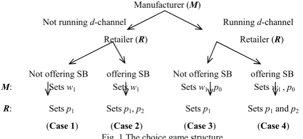
We now design the choice game between the manufacturer and the retailer unfolding in three stages. In the first stage, the manufacturer decides whether to or not to run the d-channel, and the retailer decides whether or not to complement the SB with the NB. Second, the manufacturer sets the wholesale price w1 for the NB and the online price p0 when he decides to sell direct. Finally, knowing the manufacturer’s decision, the retailer sets the NB’s price p1 at the r-channel and the SB’s price p2 if she offers the SB. There are four subgames in the model as follows: the r-channel providing only the NB (Case 1), and the r-channel providing the SB other than the NB (Case 2), introducing d-channel except the r-channel providing the NB (Case 3), r-channel introducing the SB by the retailer and d-channel being run by the NB manufacturer (Case 4). The choice game structure is illustrated in Fig. 1.
Comparing with [22], Case 3 discussed in this paper was not considered in [22]. They discussed the effect of the quality difference between NB and SB, whereas we
consider the impact of the unit operating cost difference between the NB in the d-channel and the SB. Additionally, we will focus the game’s equilibrium outcome in Section 4, Manufacturer (M)
Not running d-channel Running d-channel
M: Sets w1 Sets w1 Sets w1 , p0 Sets w1 , p0 Retailer (R) Retailer (R)
Not offering SB offering SB Not offering SB offering SB
[image:2.595.146.442.610.746.2]R: Sets p1 Sets p1, p2 Sets p1 Sets p1 and p2
Fig. 1 The choice game structure
(Case 1) (Case 2) (Case 3) (Case 4)
IAENG International Journal of Applied Mathematics, 47:1, IJAM_47_1_16
which was not discussed in [22].
Consistent with [1], assume that consumers consist of two groups: brand loyal and store loyal. The brand loyal consumers only purchase the NB from either the d-channel or the r-channel, whereas the store loyal consumers buy either the NB or the SB only from the specific retailer. The
brand loyal consumers have a strong preference for the NB and will never consider buying a different brand and the segment of size is εM. However, the store loyal consumers
are not loyal to any specific brand and the segment of size is
εR. Relative to the brand loyal consumers, the store loyal
consumers maybe be viewed as those who are less informed about the products in the specific category. They have a need to touch and feel the product before purchasing. Consequently, consumers of this type will never consider buying the NB through the d-channel.
The demand for each product and profit of each player in the four cases are summarized as follows.
Case 1: only the NB is offered in the r-channel. The demand is linear in its retail price p1, shown as follows
D=(εM+εR)(1-βp1). (1) where β measures the effect of retail price on the demand.
The linear demand function is widely applied in price competition literature (e.g., [12], [22]) since it is tractable and enables closed-form solutions.
The profits in Case 1 are given as follows
ΠM(w1)=(εM+εR)(1-βp1)(w1-c1). (2) ΠR(p1)=(εM+εR)(1-βp1)(p1-w1). (3)
Case 2: the SB and the NB are offered through the r-channel. If the SB is offered, a fraction of store loyal consumers will shift from the NB’s ones. As noted earlier store loyal consumers fulfill all their purchasing needs only in the
r-channel, the retailer could influence the purchasing decision of store loyal consumers. To capture this feature, we assume that the fraction of store loyal consumers that purchase the SB depends on the level of sales effort (e.g., advertisement and shelf space) that the retailer allocates to the SB. We assume that the total level of sales effort to SB and NB is normalized for simplicity to 1, and λ2 represents the NB’s sales effort level. Correspondingly, the SB’s sales effort is 1-λ2. The baseline demand for NB in the r-channel is equal to εM+λ2εR, and the baseline demand for SB is equal
to (1-λ2)εR. The demand for NB through the r-channel
(denoted by D1) and for the SB (denoted by D2) and the profits of the two partners are given as follows.
D1=(εM+λ2εR)(1-βp1)+η(p2-p1). (4)
D2=(1-λ2)εR(1-βp2)+η(p1-p2). (5) ΠM(w1)=[(εM+λ2εR)(1-βp1)+η(p2-p1)](w1-c1). (6) ΠR(p1,p2)=[(εM+λ2εR)(1-βp1)+η(p2-p1)](p1-w1)
+[(1-λ2)εR(1-βp2)+η(p1-p2)](p2-c2). (7) Where η is the competition intensity between NB and SB.
Case 3: the manufacturer runs the d-channel and the retailer only sells the NB. If the manufacturer runs a d-channel, a fraction of brand loyal consumers shift their purchases online. Brand loyal consumers switch from the r-channel to the d-channel due to the convenience that online shopping affords, and/or their expensive shopping (transportation) costs and/or their price sensitivities to the price. Let λ1 represent the initial ratio of the brand loyal consumers who buy the NB from the retailer to all brand loyal consumers, i.e., the baseline demand for the NB product in the
d-channel is equal to (1-λ1)εM, and the total demand for the
NB in the r-channel is equal to λ1εM +εR. The demand for the
NB through the d-channel (denoted by D0) and the demand for the NB through the retail channel (denoted by D1) are
D0=(1-λ1)εM(1-βp0)+γ(p1-p0). (8)
D1=(λ1εM+εR)(1-βp1)+γ(p0-p1). (9) Both members’ profits are
ΠM(w1,p0)=[(1-λ1)εM(1-βp0)+γ(p1-p0)](p0-c0) +[(λ1εM+εR)(1-βp1)+γ(p0-p1)](w1-c1), (10)
ΠR(p1)=[(λ1εM+εR)(1-βp1)+γ(p0-p1)](p1-w1). (11) Where γ is viewed as the channel competition intensity between the d-channel and the r-channel.
Case 4: the manufacturer runs the d-channel and the retailer offers the SB. According to Case 2 and Case 3, we assume that these demands are linearly dependent on the sales prices, which are given as follows:
(a) the brand loyal demand for NB in d-channel is
D0=(1-λ1)εM(1-βp0)+γ(p1-p0),
(b) the brand loyal demand for NB in r-channel is
D10=λ1εM(1-βp1)+γ(p0-p1),
(c) the store loyal demand for NB in r-channel is
D12=λ2εR(1-βp1)+η(p2-p1),
(d) the store loyal demand for SB in r-channel is
D2=(1-λ2)εR(1-βp2)+η(p1-p2).
The profits of the two sides are given as follows: ΠM(w, p0)=D0(p0-c0)+(D10+D12)(w-c1)
=(a0-b0p0+γp1)(p0-c0)+(a1-b1p1+γp0+ηp2)(w-c1). (12) ΠR(p1, p2)=(D10+D12)(p1-w)+D2(p2-c2)
=(a1-b1p1+γp0+ηp2)(p1-w)+(a2-b2p2+ηp1)(p2-c2). (13) where a0=(1-λ1)εM, b0=βa0+γ, a1=λ1εM+λ2εR, b1=βa1+γ+η,
a2=(1-λ2)εR and b2=βa2+η.
Due to D0+D10+D12+D2=(1-λ1)εM(1-βp0)+(λ1εM+λ2εR)
(1-βp1)+(1-λ2)εR(1-βp2), the total demand is not affected by γ and η. This implies that a change in intensities of both channel competition and brand competition do not lead to any variation in the aggregate demand.
III. TWO MEMBERS’DECISIONS IN EACH CASE
Case 1: only NB available through the r-channel
As a benchmark, we develop a basic model where neither the manufacturer runs the d-channel nor the retailer introduces SB (denoted by superscript “n”). As the leader, the manufacturer first declares w1, the retailer then decides her retail price p1. From (2) and (3), one can derive by backward induction that the prices and the profits are
w1n=c1+(1-βc1)/(2β),
p1n = c1+3(1-βc1)/(4β), ΠMn=(εM+εR)(1-βc1)2/(8β),
ΠRn=(εM+εR)(1-βc1)2/(16β). (14) Case 2: only introducing the SB
In this setting, only the retailer introduces the SB, and the profits for both sides are respectively given in (6) and (7). One can derive two members’ optimal pricing strategies (denoted by superscript “s”). Lemma 1 gives the optimal pricing strategies for both members.
Lemma 1. Define m=b0+b1-2γ, if only the retailer sells the SB, then the optimal pricing strategies are given by
p1s = c1+3(1-βc1)/(4β)-η(1-βc2)/(4βm),
p2s= c2+(1-βc2)/(2β),
w1s= c1+(1-βc1)/(2β)-η(1-βc2)/(2βm).
All proofs are provided in Appendix. From Lemma 1, one
IAENG International Journal of Applied Mathematics, 47:1, IJAM_47_1_16
can easily derive that the market demands of the two products and the profits of two sides are given as follows:
D1s= m(1-βc1)/(4β)-η(1-βc2)/(4β),
D2s= (2b2m-η2)(1-βc2)/(4βm)-η(1-βc1)/(4β), ΠM s=[m(1-βc1)-η(1-βc2)]2/(8β2m),
ΠRs=(4b2m-3η2)(1-βc2)2/(16β2m)-η(1-βc1)(1-βc2)/(8β2)
+m(1-βc1)2/(16β2). The differences of the wholesale prices and the retail prices between Case 1 and Case 2 are as follows:
w1s-w1n= -η(1-βc2)/(2βm)<0,
p1s-p1n=-η(1-βc2)/(4βm)<0.
The wholesale price and the retail price of the NB in Case 2 are lower than that in Case 1. This implies that introducing the SB induces the decreasing of the wholesale price and the retail price for NB. As a result, the manufacturer’s profit margin for the NB is reducing. However, an interesting phenomenon is that the retailer’s profit margin for NB is increasing due to (p1s- w1s)-(p1n-w1n)=η(1-βc2)/(4βm)>0. Table 1 Sensitivity of pricing strategies to the parameters in Case 2
c2 η λ2 εM εR
w1s + - + + + p2d + 0 0 0 0 p1d + - + + +
The sensitivity of the pricing strategies to the parameters is listed in Table 1. When c2 increases, the SB’s price increases. The higher the SB’s cost, the weaker the SB’s competition with the NB will be. Correspondingly, the manufacturer increases the wholesale price and the retailer increases the retail price. The higher the competition intensity (η) between the NB and the SB, the lower the wholesale price and the retail price is. When the brand loyal consumers (εM), or the store loyal consumers (εR) or the
initial ratio of the store loyal consumers who prefer to buy the NB (λ2) increase, the NB’s baseline demand increases and, hence, the manufacturer increases the wholesale price and the retailer will increase the NB’s retail price.
Theorem 1 gives the condition under which the retailer is willing to introduce the SB, and the impact of introducing the SB on the profits for the manufacture, the retailer and the whole supply chain.
Theorem 1. (1) if c2[c2s-min, c2s-n], the retailer is willing to introduce the SB;
(2) if c2[c2s-min, c2s-n], then ΠRs≥ΠRn and ΠMs≤ΠMn;
(3) if c2[c2s-min, c2C-s), then ΠCs=ΠRs+ΠMs>ΠCn=ΠRn+ΠMn,
and if c2[c2C-s, c2s-n], thenΠCs≤ΠCn, where
c2s-min =max[(η-m(1-βc1))/(βη),0];
c2s-n = min{1/β-mη(1-βc1)/[β(2b2m-η2)],1/β-[mη+√(m2η2 -m(b2-2η)(4b2m-3η2)](1-βc1)/[β(4b2m-η2)]};
c2C-s=1/β-[3mη(1-βc1) +√(9m2η2-3(4b
2m-η2)(b2-2η))](1-βc1)/[β(4b2m-η2)]. From Theorem 1, we obtain that the retailer can benefit from the introduction of the SB, whereas the manufacturer will be worse off in the presence of the SB. Besides, the brand competition between the two partners benefits to the supply chain only if the unit cost of SB is low, i.e., c2<c2C-s, correspondingly, Pareto improving is achieved, whereas the brand competition harms the supply chain if c2>c2C-s. Case 3: only running introducing the d-channel
In this case, only the manufacturer runs the d-channel, and the profits of both sides are given in (10) and (11). Two
members’ optimal pricing strategies are shown in Lemma 2 (denoted by superscript “d”).
Lemma 2. Define k=b1+b2-2η, if the manufacturer runs the
d-channel, then the optimal pricing strategies are given by
p1d= c1+3(1-βc1)/(4β)-γ(1-βc0)/(4βk),
w1d= c1+(1-βc1)/(2β),
p0d=c0+(1-βc0)/(2β).
It is easy to have p0d-w1d=(c0-c1)/2≥0 due to c0≥c1. This means that when the manufacturer runs the d-channel, the manufacturer’s online price is no less than his wholesale price offered to the retailer, which means that the retailer will not purchase the NB from the d-channel.
From Lemma 2, one easily derives that the demands and the profits of two members are respectively given by
D0d =(2b0k-γ2)(1-βc0)/(4βk)-γ(1-βc1)/(4β),
D1d =k(1-βc1)/(4β)-γ(1-βc0)/(4β),
ΠM d=(2b0k-γ2)(1-βc0)2/(8β2k)-γ(1-βc0)(1-βc1)/(4β2) +k(1-βc1)2/(8β2),
ΠR d=[k(1-βc1)-γ(1-βc0)]2/(16β2k).
Comparing the wholesale price and the retail price between Case 1 and Case 3 leads to:
w1d-w1n=0,
p1d-p1n=-γ(1-βc0)/(4βk)<0.
Note that the wholesale price for the NB in Case 1 and Case 3 is equal, whereas the retail price in the r-channel in Case 3 is lower than the one in Case 1. This implies that running the d-channel forces the retailer to decrease the retail price. Correspondingly, her profit margin is decreasing. This indicates that the channel competition harms the retailer, benefits consumers, and weakens the negative effects of double marginalization caused by high retail price. Table 2 lies in the sensitivity of the pricing strategies in Case 3 with respect to the parameters. The direct price and the retail price for the NB increase with the operating cost of
d-channel (c0). If the channel competition intensity (γ) between the d-channel and the r-channel increases, the retailer has to decrease the NB’s price. When the brand
loyal consumers (εM), or the store loyal consumers (εR) or
the initial ratio of the brand loyal consumers who prefer to buy the NB from the retailer (λ1) increase, the baseline demand for the NB at the r-channel increase and, hence, the retailer will increase the NB’s retail price.
Table 2 Sensitivity of pricing strategies to the parameters in Case 3 c0 γ λ1 εM εR
w1d 0 0 0 0 0 p0d + 0 0 0 0 p1d + - + + +
The specified condition under which the manufacturer is willing to run the d-channel is discussed as follows.
Theorem 2. (1) if c0[c1, c0d-n], the manufacturer is willing to run a d-channel;
(2) if c0[c1, c0d-n], then ΠMd≥ΠMn and ΠRd≤ΠRn;
(3) if c0[c1, c0C-d), then ΠCd>ΠCn, and if c0[c0C-d, c0d-n], then ΠCd<ΠCn, where
c0s-max= min{1/β -γk(1-βc1)/[β(2b0k-γ2)],1/β-[γk+√(k2γ2 -k(b0-2γ)(2b0k-γ2)](1-βc1)/[β(4b0k-γ-2)]};
c0C-d=1/β-[3 kγ(1-βc1)
+√(9k2γ2-3(4b0k-γ2)(b0-2γ))](1-βc1)/[β(4b0k-γ2)]. From Theorem 2, we can obtain that the manufacturer can benefit from running the d-channel, whereas the retailer will
IAENG International Journal of Applied Mathematics, 47:1, IJAM_47_1_16
be worse off from running the d-channel. Besides, the channel competition between the two partners benefits to the supply chain only if the unit cost in the d-channel is low than c0C-d, i.e., c0<c0C-d, correspondingly, Pareto improving is achieved.
Case 4: running the d-channel and introducing the SB
If the manufacturer runs the d-channel and the retailer introduces the SB, the profits are given in (12) and (13). One can derive two members’ optimal pricing strategies (denoted by the superscript “ds”). Lemma 3 gives the optimal pricing strategies for both sides.
Lemma 3. Define n=(2b1b2-η2)(b0b1-γ2)-η2b0b1, if the
d-channel and the SB occur simultaneously, the optimal pricing strategies for both members are given by
p1ds= c1+3(1-βc1)/(4β)-γb2(1-βc0)/[4β(b1b2-η2)] -ηb0(b1b2-η2)(1-βc2)/(2βn),
p2ds= c2+(1-βc2)/(2β)-γη(1-βc0)/[4β(b1b2-η2)] -γ2η2(1-βc
2)/(4βn),
w1ds = c1+(1-βc1)/(2β)-η[2b0(b1b2-η2)-γ2b2](1-βc2)/(2βn),
p0ds = c0+(1-βc0)/(2β)-γη(b1b2-η2)(1-βc2)/(2βn).
The optimal pricing policies will lead to the demands of two products in the two channels below.
D0ds= [2b0(b1b2-η2)- γ2b2](1-βc0)/[4β(b1b2-η2)] -γ(1-βc1)/(4β);
D1ds= [b1(1-βc1)-γ(1-βc0)-η(1-βc2)]/(4β);
D2ds=b2(1-βc2)/(4β)+(b1b2-η2)(b0b1b2-γ2b2-η2b0)(1-βc2) /(2βn)-η(1-βc1)/(4β);
Since c0≥c1, it is obvious to have p0ds-w1ds≥0. That is to say, when the manufacturer runs the d-channel and the retailer introduces the SB as well, the manufacturer’s online price in the d-channel is no less than his wholesale price offered to the retailer and, hence, the retailer will not purchase the NB product from the d-channel.
From the above analyses, we can derive Lemma 4.
Lemma 4. (1) p1ds≤ p1s≤ p1n, p1ds≤ p1d ≤ p1n, p0ds≤ p0d and
p2ds≤ p2s;
0 0 2 2
(2) Md 0, Mds 0, Ms 0, Mds 0;
c c c c
2 2 0 0
(3) 0, 0, 0, 0.
s ds d ds
R R R R
c c c c
Lemma 4 indicates that the channel and the brand competition induce the decreasing of retail prices. This means that the competition benefits consumers, increases the total demand and, hence, weakens the negative effects of double marginalization. From Lemma 4, one can also observe that if the manufacturer runs the d-channel, his profit will decrease but the retailer’s will increase as the unit operating cost in the d-channel increases. Likewise, if the retailer introduces the SB, her profit will decrease but the manufacturer’s profit will increase as the unit purchasing cost of the SB increases.
We will discuss under what condition the manufacturer will run the d-channel given that the retailer has introduced the SB, and under what condition the retailer will introduce the SB given that the manufacturer has run the d-channel.
Suppose that the retailer has introduced the SB (i.e., the parameter c2 is given). In that case, if the manufacturer wants to run a d-channel, a fundamental condition is to assure D0ds≥0, which is equivalent to
2
max
1 2 1
0 2 2 0
0 1 2 2
( )(1 )
1
[2 ( ) ]
ds
b b c
c c
b b b b
.
Besides, it is also necessary to pledge the manufacturer’s profit increment incurred by running the d-channel no less than zero. Denote this increment by △ΠMds-s(c0|c2), then
2 2
0 1 2 2 2
0 2 2 2 0
1 2
2 ( )
( | ) (1 )
8 ( )
ds s M
b b b b
c c c
b b
2 01 0 1
2 2
2
2 2 2
1 2 0 2 2 2
2
(1 )(1 ) (1 )
4 8
2( ) (1 ) .
8
b
c c c
b b b b m n c
nm
ΠMs is constant with respect to c0, and ΠMds decreased
with c0 according to Lemma 4. Thus, △ΠMds-s(c0|c2) decreases with c0. Hence, if △ΠMds-s(c0ds|c2)≥0, then
c0ds-max is the maximal unit operating cost (denoted by
c0ds-s) that the manufacturer can run the d-channel. Otherwise, if △ΠMds-s(c1|c2)>0, then the equation
△ΠMds-s(c0|c2)=0 will be a unique root (denoted by c01(c2)) in the interval (c1, c0ds-max), whereas △ΠMds-s(c1|c2)≤0 is more beneficial for the manufacturer not to run the
d-channel. To sum up, given that the retailer has introduced the SB, the condition that the manufacturer should run the d-channel is that his unit operating cost in the d-channel does not exceed c0ds-s, where
max max
0 0 2
0 1 max
0 2 1 2 0 2
, | 0,
, | 0 | .
ds ds s ds
M ds s
ds s ds s ds
M M
c c c
c
c c c c c c
Given that the manufacturer has run the d-channel, a fundamental condition for the retailer selling the SB is to have D2ds≥0, which is equivalent to
1 1
max2 2 2 2 2
1 2 1 2
1 1 . ( )( ) ds nb c c c
nb b b b n
, i.e., c0ds-s=c0ds-max;
Additionally, it is also natural to have the retailer’s profit increment incurred by selling the SB product no less than zero. Denote this profit increment of the retailer by
△ΠRds-d(c2|c0), then
21 2 1 2 2 2 2 2 2 22 0 2 2 2
1
( )( )(3 )
| (1 )
16 ds d
R
n b b b b n n
c c c
n b 2 2
0 2 1 2
2 2
1
( )
(1 )(1 ) (1 )(1 )
8 8
n
c c c c
nb 2 2 2 2 2 2 1 0
2 2 2
1 2
( 2 )(1 ) ( ) (1 ) .
16 16 ( )
b c b c
k b b
Noting that ΠRd is constant with respect to c2 and ΠRds is a
decreasing function of c2 due to Lemma 4, we have that
△ΠRds-d(c2|c0) is a decreasing function of c2. Therefore, if
△ΠRds-d(c2ds-max|c0)≥0, then c2ds-maxwill be the maximal unit operating cost that the retailer can introduce the SB, otherwise, the equation △ΠRds-d(c2|c0)=0c2ds-d will be a unique root (denoted by c21(c0)) in (c1, c2ds-max) because
△ΠRds-d(c1|c0)>0, which will be derived in Appendix. Summing up the above analysis, we have that, given that the manufacturer has run the d-channel, the condition that the retailer introduce the SB is that her unit operating cost for the SB does not exceed c2ds-d, where
max
2 2 0
0 1
2 0 2 0
, | 0,
, | 0.
ds ds d ds
R ds d
ds d ds R
c c c
c
c c c c
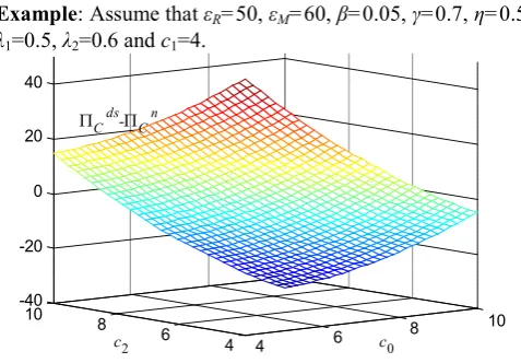
However, it is difficult to discuss theoretically the impact of the SB and running the d-channel on the whole supply chain’s profit. We use a numerical example to illustrate how the parameters c0 and c2 affect the supply chain’s profit.
IAENG International Journal of Applied Mathematics, 47:1, IJAM_47_1_16
Example: Assume that εR=50, εM=60, β=0.05, γ=0.7, η=0.5,
λ1=0.5, λ2=0.6 and c1=4.
4 6 8
10 4
6 8 10 -40 -20 0 20 40
c0 c2
[image:6.595.49.288.50.216.2]Cds- Cn
Fig.2 The profit increment by running d-channel and SB
Fig. 2 shows that the profit difference between Case 4 and Case 1 varies with the parameters c0 and c2. From Fig. 2, we can conclude that when with both c0 and c2 are low, introducing SB and running a d-channel can achieve the whole chain’s performance, and Pareto improving, which is consistent with that discusses in Case 2 and Case 3.
IV. BOTH MEMBERS’ CHOICE GAME
Section 3 has shown two members’ option behaviors given the action of their individual adversary. In this section, we will discuss their Nash equilibrium options.
In the mS framework, the manufacturer first determines whether to run a d-channel and he has two possible strategies: “Yes” and “No” (denoted by {Y} and {N} for brevity, respectively). “{Y}/{N}” means “running/not running a d-channel”. As a follower, the retailer’s action depends on the manufacturer’s strategy. Thus, she has four possible policies: {Y, Y}, {Y, N}, {N, Y} and {N, N}. {Y, N} represents that the retailer introduces SB if the manufacturer runs the d-channel, and introduce SB without the d-channel. {N, Y} is contrary to {Y, N}. {Y, Y} means that the retailer always introduces the SB whether or not the manufacturer runs the d-channel. {N, N} is contrary to {Y, Y}. Thus, the choice game between the two partners has eight possible strategy profiles: ({Y}, {Y, Y}), ({Y}, {Y, N}), ({Y}, {N, Y}), ({Y}, {N, N}), ({N}, {Y, Y}), ({N}, {Y, N}), ({N}, {N, Y}) and ({N}, {N, N}). In each strategy profiles, the first element is the manufacturer’s action and the second one is the retailer’s action. The two strategies ({Y}, {Y, Y}) and ({Y}, {Y, N}) induce the same outcome (Y, Y) i.e., the manufacturer runs the d-channel and the retailer introduces the SB. Therefore, there are four possible equilibrium outcomes: (Y, Y), (Y, N), (N, Y) and (N, N). Table 3 shows the payoff matrix of two players.
Table 3 Payoff matrix of the two players Retailer
{Y,Y} {Y,N} {N,Y} {N,N} {Y} (ΠMds, ΠRds) (ΠMds, ΠRds) (ΠMd, ΠRd) (ΠMd, ΠRd)
Manu..
{N} (ΠMs, ΠRs) (ΠM*, ΠR*) (ΠMs, ΠRs) (ΠM*, ΠR*)
From Table 3 and the analyses in Sections 3, we can derive the Nash equilibrium options according to the parameters c0 and c2, which are shown as follows.
(1) If c2≤ min{c2s-n, c2ds-d}, then the retailer’s strategy is {Y, Y}. In such a case, if the manufacturer introduces the
d-channel, his profit is ΠMds; otherwise, his profit is ΠMs.
Thus, the manufacturer chooses the d-channel if and only if ΠMds>ΠMs, i.e., c0<c0ds-s. From the above analysis, the Nash equilibrium is (Y, Y) for c0<c0ds-s and c2≤min{c2s-n,c2ds-d}, and (N, Y) for c0≥c0ds-sand c2≤ min{c2s-n,c2ds-d}.
(2) If c2s-n<c2≤c2ds-d, the retailer’s strategy is {Y, N}. This means that she will introduce the SB if the manufacturer runs the d-channel, but she will not introduce the SB if the manufacturer does not sell online. In such a case, if the manufacturer introduces the d-channel, his profit is ΠMds;
otherwise, his profit is ΠMn. Thus, the manufacturer
introduces the d-channel only if ΠMds>ΠMn. Obviously, ΠMn
is constant with respect to c0, and ΠMds is a decreasing
function of c0 according to Lemma 4. We have that △ ΠMds-n(c0|c2)=ΠMds-ΠMn is a decreasing function of c0. Thus, if △ΠMds-n(c0ds-max|c2)≥0, then c0ds-max will be the maximal unit operating cost that the manufacturer runs the
d-channel, otherwise, the equation △ΠMds-n(c0|c2)=0will be a unique root (denoted by c0(2)(c2)). To sum up, the Nash equilibrium is (Y, Y) for c0<c0ds-nand c2s-n<c2≤c2ds-d, and (N, N) for c0≥c0ds-nand c2s-n<c2≤c2ds-d, where
max
0 0 2
0 ( 2)
0 2 1 2 0 2
, ( | ) 0 ,
( ), ( | ) 0 ( | ).
ds ds n ds
ds n M
ds n ds n ds
M M
c c c
c
c c c c c c
(3) If c2ds-d<c2≤c2s-n, the retailer’s strategy is {N, Y}. In such a case, if the manufacturer introduces the d-channel, his profit is ΠMd, otherwise, his profit is ΠMs. Thus, the
manufacturer is willing to introduce the d-channel only if ΠMd>ΠMs. ΠMs is constant with respect to c0, and ΠMd is a
decreasing function of c0 in Case 2. Thus △ΠMd-s(c0) =ΠMd-ΠMs is a decreasing function of c0. Therefore, if △ ΠRd-s(c0d-max)≥0, then c0d-max will be the maximal unit operating cost that the manufacturer can introduce the
d-channel, otherwise, the equation △ΠMd-s(c0)=0 will be a unique root (denoted by c0(2)) for c0(c1, c0d-max). To sum up, we have that, the Nash equilibrium is (Y, N) for c0<c0d-sand
c2ds-d<c2≤c2s-n, and (N, N) for c0≥c0d-sand c2ds-d<c2≤c2s-n,
2
max 0
0 2 1 2
0 0
(2) 0
2( )
, 1 (1 )
where 2
, d d s
b k
c m mk c c
c b k
c otherwise
1(2)
0 2
0
1 1 and
2
km c
c
b k m
2
2 2 2 2 2
0 1 2 0 1
2 0
2 [ (1 ) (1 )] 2 1
. 2
b k km m c c b k k m c
b k m
(4) If c2>max{c2s-n, c2ds-d}, the retailer’s strategy is {N, N}. This means that if the manufacturer introduces the
d-channel, his profit is ΠMd, otherwise, his profit is ΠMn.
Thus, the manufacturer chooses the d-channel if and only if ΠMd>ΠMn, i.e., c0<c0d-n. Consequently, the Nash equilibrium is (Y, N) for c0<c0d-n and c2>max{c2s-n, c2ds-d}, and (N, N) for c0≥c0d-nand c2>max{c2s-n, c2ds-d}.
The above analyses show that the equilibrium options are dependent on the unit operating cost (c0) of the d-channel and the SB’s unit operating cost (c2). We can conclude that the retailer’s optimal option is to introduce the SB if c2 is relatively low, whereas she does not introduce the SB if it is relatively high. If c2 is medium, the retailer’s optimal policy depends on the manufacturer’s decision. Thus the manufacturer has the advantage of making the first move, and it is possible that he can choose the policy which
IAENG International Journal of Applied Mathematics, 47:1, IJAM_47_1_16
maximizes his profit, but may be harmful to the retailer. Besides, if c0 and c2 are very low (i.e., c0<c0ds-s and c2≤ min{c2s-n, c2ds-d}), the optimal choice is (Y, Y), whereas if
c0 and c2 are very high (i.e., c0>c0d-n and c2>max{c2s-n,
c2ds-d}), the choice game’s outcome is (N, N). This is consistent with our intuition.
5 10 15
[image:7.595.69.264.124.468.2]13.5 13.6 13.7 13.8
Fig. 3.1 Variation of c2ds-dand c2s-n with c0 c2s-n
c2ds-d
4 6 8 10 12 14 16
5 10 15
Fig. 3.2 Variation of c0d-sand c0ds-n with c2
c0d-s c0ds-n
4 6 8 10 12 14 16
9.98 10 10.02
Fig. 3.3 Variation of c0ds-sand c0d-n with c2 c0d-s
c0d-n
c0ds-s
We use numerical examples to further illustrate how the two players determine their equilibrium options. The value of these parameters is also consistent with that in the above example in Case 4, Section 3.
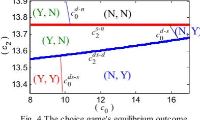
Fig. 3.1 shows how c2s-n and c0ds-d change with the parameter c0,andthe horizontal axis represents c0. From Fig. 3.1, we see that c2s-n>c2ds-d. Fig. 3.2 and Fig. 3.3 indicate how c0d-s, c0ds-n, c0ds-s and c0d-n change with parameter c2, respectively, and the horizontal axis represents parameter c2. If the manufacturer runs the d-channel, the retailer introduces the SB only if c2<c2ds-d; otherwise, the retailer introduces SB only if c2<c2s-n. This means that running the
d-channel may decrease the possibility of introducing SB. According to the above analyses and Figs. 3.1-3.3, we can induce the equilibrium outcome for the two players, which is shown in Fig. 4. From Fig. 4, we can observe that the optimal equilibrium outcome is (Y, Y) if c0<c0ds-s and
c2<c2ds-d<c2s-n, and (N, Y) if c0>c0ds-s and c2<c2ds-d<c2s-n. This is because that c2<c2ds-d<c2s-n induces the retailer’s optimal choice {Y, Y}, which means that the manufacturer’s choice does not affect the retailer’s strategy. Given the retailer’s optimal strategy, the manufacturer should choose to run the d-channel if c0<c0ds-s, and not to run the d-channel if c0>c0ds-s. Similarly, the equilibrium outcome is(Y, N) if
c0<c0d-s and c2ds-d<c2<c2s-n, and (N, Y) if c0>c0d-s and
c2ds-d<c2<c2s-n. The outcome is (Y, N) if c0<c0d-n and c2ds-d
<c2s-n<c2, and (N, N) if c0>c0d-n and c2ds-d<c2s-n<c2. From Fig. 4, we maybe conclude that the equilibrium outcome is (Y, Y) for low c0 and low c2, and (N, N) for high c0 and high c2, and (N, Y) for high c0 and low c2, and (Y, N) for low c0 and high
c2. However, for medium c0 and medium c2, the equilibrium outcome is (Y, N). In such a case, the retailer’s choice will depend on the manufacturer’s strategy. As the choice game’s leader, the manufacturer has the advantage of the first move, and he prefers to run the d-channel.
8 10 12 14 16
[image:7.595.327.524.162.280.2]13.4 13.5 13.6 13.7 13.8 13.9
Fig. 4 The choice game's equilibrium outcome
(
c 2
) c2
s-n
c2ds-d
( c0 )
(Y, Y) (N, Y)
(N, N) c0d-n
(Y, N)
c0ds-s
(Y, N) c0d-s (N, Y)
We will discuss how the parameters c0 and c2 influence the players’ profit increments derived from their optimal options. Let ΠR*, ΠM* and ΠC*(=ΠR*+ΠM*)be the retailer’s
profit, the manufacturer’s profit and the supply chain profit under the optimal strategies, respectively. For example, from Fig. 4, the optimal equilibrium outcome is (Y, Y) if
c0=7 and c2=5. In such a case, we have that ΠR*=ΠRds,
ΠM*=ΠMds and ΠC*=ΠCds =ΠRds+ΠMds.
Fig. 5 shows how the profit increments vary with c0 given
c2=5, c2=13.7 and c2=15, respectively, and the horizontal axis represents parameter c0. From Fig. 5, we can observe that the increase of c0 is always adverse to the manufacturer but beneficial to the retailer, whereas the increase of c2 is always harmful to the retailer but profitable to the manufacturer. This means that the manufacturer (the retailer) should lower the unit operating cost c0 (c2) to enhance competitive power in introducing the d-channel (the SB). From supply chain perspective, the increase of c0 (c2) is always adverse to the whole chain. Another observation from Fig. 5 is that when both c0 and c2 are relatively smaller (say, c0≤6 and c2=5 in the leftmost part of Fig. 5), the three profit increments ΠR*-ΠRn, ΠM*-ΠMn and ΠC*-ΠCn all remain
non-negative. This indicates that when the operating costs of both the d-channel and the SB are not very high, the two parties’ game of introducing the d-channel and the SB product leads to an increase of both players’ profits and the whole channel profit as well. This also implies that the two parties’ competition on introducing the d-channel and the SB can eliminate the negative effects of double marginalization, which is further verified by the fact that the competition induces lower pricing of both the manufacturer and the retailer (shown in Lemma 4).
In order to illustrate how parameters εM,εR,λ1, λ2, γ and η influence the two parties’ profits, respectively, we present the sensitivity analysis of the two parties’ profits with respect to these parameters. The initial parameter values are those assumed in Example except for c0=7 and c2=5. We carry out the analysis by increasing the value of one single parameter by -50% up to 50% while holding all the other parameters constant. Fig. 6 shows that how the changes of
εM,εR,λ1, λ2, γ and η influence two parties’ profits.
IAENG International Journal of Applied Mathematics, 47:1, IJAM_47_1_16
5 10 15 -40
-20 0 20 40 60
T
he
p
rof
it
i
nc
re
m
ent
s
5 10 15
-40 -20 0 20 40 60
5 10 15
-40 -20 0 20 40 60
R*-Rn C*-Cn
M*-Mn
C*-
C n
R*-
R n
M*-Mn
c0 (c2=15)
c0 (c2=13.7)
c0d-n
c0 (c2=5) C*-
C n
R*-
R n
M*-
M n
c0ds-s c
0
[image:8.595.98.494.51.350.2]d-s
Fig. 5 The impact of c0 and c2 on profit increments
-50 0 50
100 120 140 160 180 200 220
Parameters change (%)
T
he
m
an
uf
ac
tu
re
r'
s
pr
of
it
-50 0 50
60 80 100 120 140 160 180
Parameters change (%)
T
he
r
et
ai
le
r'
s
pr
of
it
M R
1 2
Fig. 6 Impact of M , R , , , 1and 2 on two players' profits Fig.6 gives the following conclusions.
(1) The manufacturer’s/retailer’s profit increases as either
εM orεR increases. That is, the increase of the market size for
manufacturer loyalty or retailer loyalty is beneficial to both the retailer and the manufacturer, which is explained by the fact that the increase of εM orεR leads to the arising of the
total market demand.
(2) The retailer’s profit increases as parameters λ1 and η increase but decreases as λ2 and γ increase, whereas the manufacturer’s profit decreases as parameters λ1 and η increase but increases as λ2 and γ increase. This indicates that (i) the higher the proportion of the brand loyal consumers who buy NB from the r-channel, the more beneficial to the retailer but the more harmful to the manufacturer; (ii) the greater the proportion of the store
loyal consumers who prefer the NB product, the more profitable to the manufacturer but the more harmful to the retailer; (iii) the fiercer the channel competition, the more beneficial to the manufacturer but the more harmful to the retailer, whereas it is just reverse for the brand competition. The former two points are consistent with our expectation. They imply that when the manufacturer competes for both channel and brand with the retailer, the manufacturer should strive to expand d-channel loyalty but also attract more store
loyal customers buying the NB product, whereas the retailer should build up the SB loyalty and attract more brand loyal customers buying from the r-channel. The last one implies that the manufacturer should strengthen channel competition whereas the retailer should increase the brand competition.
V. DISCUSSION AND IMPLICATIONS
A. Theoretical contributions
The prior literature mainly focused on dual-channel supply chains (Kumar and Ruan, 2006[1], Wang et al. 2016[2],
Chiang et al. (2003)[4]), ignoring the introduction of the SB, whereas, most of the literature on the SB ignored the channel competition between the r-channel and the
d-channel. This study has concentrated on a choice game in which whether a manufacturer runs a d-channel and whether a retailer should respond by introducing the SB, thereby enriching literature in this area. The theoretical contributions of this paper are shown as follows.
Corroborating the studies (Amrouche and Yan (2012)[22]; Shang and Yang (2015)[14]; Kurata et al. (2007)[21]), running the d-channel and introducing the SB has been found to cause the competition between the manufacturer and the retailer, and to exert significant influence on pricing strategies for the two partners as well. It reaffirms the argument that the competition forces the firms to reduce pricing. It is therefore not surprising to see that the competition between the firms can weaken the negative effects of double marginalization on the overall supply chain profit, and increase more consumer surpluses.
With the absence of the SB, running a d-channel benefits the manufacturer (Kumar and Ruan, 2006[1], Cai et al. (2009)[12]). Similarly, Without running a d-channel, the retailer can be better off through introducing SBs (Pauwels and Srinivasan, 2004[8], Narasimhan and Wilcox (1998) [17]). Our study suggests that the operating cost in the
d-channel and the SB operating cost have been found to exert a significant influence on the strategies and the profits for the manufacturer and the retailer. Specifically, when the
d-channel’s operating costs and the SB’s operating costs are small, running a d-channel and introducing a SB can benefits the manufacturer and the retailer, whereas when the costs are high, it is contrary.
B. Implications for practice
With economic globalization and rapid development of
IAENG International Journal of Applied Mathematics, 47:1, IJAM_47_1_16
Internet, interest in establishing a d-channel has grown explosively among manufactures in recent years. However, opportunities and threats exist when the d-channel is established in addition to existing r-channels. Meanwhile, in consumer goods retailing, the SB is threatening the NB. This study has focused on channel selection and brand choice between the manufacturer and the retailer. The findings provide recommendations to the two partners in decision- making.
Both of the manufacturer and the retailer should strive to expand the market and increase the market size. For the manufacturer, he should strive to expand d-channel loyalty to increases brand loyal customers, and strengthen the channel competition between d-channel and r-channel. However, for the retailer, our finding suggests that the retailer should strive to expand store loyalty to increases
r-channel loyal customers, and strengthen the brand competition between the NB and the SB.
VI. CONCLUSIONS
This paper discusses both channel competition and brand competition issues in a two-echelon supply chain, where a dominant manufacturer sells a NB through a retailer. Besides the r-channel, the manufacturer may select a
d-channel. Likewise, the retailer may choose a SB. We study the two partners’ optimal strategies. The results show that (i) the competition between channels or brands can weaken the negative effects of double marginalization, and (ii) when the operating costs for the d-channel and the SB are relatively low, a win-win equilibrium outcome can be achieved, which is not the case when the operating costs are relatively high. The sensitivity analyses reveal that the retailer should build up the product loyalty for the SB and increase the substitutability between the SB and the NB, whereas the manufacturer should build up the loyalty for
d-channel and decrease the substitutability between the SB and the NB, which can be achieved by increasing product differentiation.
Future research may include two aspects. First, this paper only investigated the aspect of price. It would be interesting to introduce other marketing elements in the model, such as advertising, and shelf-space allocation. Second, this model considers deterministic demand and symmetric information. Stochastic demand and information asymmetry are challenging and interesting.
APPENDIX
Proof of Lemma 1. From (6), we have R is a concave function
with respect to (p1, p2). Solving the first-order conditions gives
1 2
1 2
1 , 1 . ( .1)
2 2
s w s c
p p A
Substituting (A.1) to (7) gives the manufacturer’s profit as:
1 2
1 1 1
(1 ) (1 )
( ) ( ). ( .2)
2 M
m w c
w w c A
From (A.2), one easily derives thatdM( ) /w1 dw1 m 0. Thus w1s= c1+(1-βc1)/(2β)-η(1-βc2)/(2βm). (A.3)
Substituting (A.3) to (A.1) gives p1s, w1s and p2s.
Proof of Theorem 1. (1) One easily derives that D1s≥0 and D2s ≥0 are equivalent to max[(η-m(1-βc1))/(βη),0]c2s-min ≤c2 ≤c2s-max1/β-ηm(1-βc1)/[β(2b2m-η2)]. It implies that the retailer or the manufacturer or will exit when c2[c2s-min, c2s-max]. We do not
consider the situation where any of the two members exits. Hence, we restrict c2[c2s-min, c2s-max]. For c2[c2s-min, c2s-max], the retailer’s profit increment is given by
△ΠRs-n(c2)=[(4b2m-3η2)(1-βc2)2-2mη(1-βc1)(1-βc2) -m(b2-2η)(1-βc1)2]/(16β2m).
The retailer will introduce the SB as long as Π△ Rs-n(c2)>0. △
Since d ΠRs-n(c2)/dc2=-D2s<0 for c2s-min ≤c2≤c2s-max, Π△ Ms-n (c2) is decreasing with c2. (2b2m-η2)(b2-2η)+m2η4<0 derives △ΠRs-n
(c2s-max)>0. Hence, the monotonicity of △ΠMs-n(c2) means that △ΠRs(c2)>0 keeps in [c2s-min, c2s-max]. If (2b2m-η2)2 (b2-2η)+m2η4≥0,
△
it is clear to have ΠRs-n(c2s-max)≤0. In that case, due to c2s-min<c1, △ΠRs-n(c1)=(b2m-η2)(1-βc1)2 /(8β2m)>0 and the monotonicity of △ΠRs-n(c2), the equation △ΠRs-n(c2)=0 has a unique zero-point in [c2s-min, c2s-max]. Solving Π△ Rs-n(c2)=0 will give c2(1) as the unique zero-point in the interval [c2s-min, c2s-max]. Therefore, Π△ Rs-n(c2) >0 will hold in the interval [c2s-min, c2(1)], where
c2(1)=1/β-[mη+√(m2η2-m(b2-2η)(4b2m-3η2)](1-βc1) /[β(4b2m-η2)]}.
Define c2s-n= min{ c2s-max, c2(1)}, then the retailer introduces the SB if and only if c2 [c2s-min, c2s-max].
(2) For c2 [c2s-min, c2s-n], then ΠRs>ΠRn. The manufacturer’s profit
increment is
△ΠMs-n(c2)= [m(1-βc1)-η(1-βc2)]2/(8β2m)-(m+b2-2η)(1-βc1)2/(8β2). △
Due to d ΠMs-n(c2)/dc2=ηD1s/(2m)>0, Π△ Ms-n(c2) is an increasing function of c2 in [c2s-min, c2s]. Since c2s-n≤c2s-max, for c2s-min≤c2≤c2s-n we have
△ΠM s-n(c2)△ΠM s-n(c2s-n) △ΠMs-n(c2s-max)
2 2 4
2 2 2 1
2 2 2
2
[4 ( )( ) ( 2 )](1 )
= 0.
8 (2 )
m b m b m b c
b m
(3) The chain’s profit increment is given by
△ΠCs-n(c2)=(4b2m-3η2)(1-βc2)2/(16β2m)-3η(1-βc1)(1-βc2) /(8β2)-3(b
2-2η)(1-βc1)2/(16β2).
△ΠCs-n(c1)=(b2m-η2)(1-βc1)2/(16β2m)>0, and △ΠCs-n(c2s-n)<0 (due to ΠRs(c2s-n)=ΠRnand ΠMs(c2s-n)< ΠMn ). Thus, △ΠCs-n(c2) has the unique zero-point in (c1, c2s-max) because Π△ Cs-n(c2) is a quadratic function on c2. Solving △ΠCs-n(c2)=0 gives the unique zero-point c2C-s, of Π△ Cs-n(c2) in the interval (c1, c2s-max) as
c2C-s =1/β-[3mη(1-βc1) +√(9m2η2-3(4b
2m-η2)m(b2-2η))](1-βc1)/[β(4b2m-η2)]. △
Thus, it derive that ΠCs-n(c2)>0 for c2(c2s-min, c2C-s) and △ΠCs-n(c2) <0 for c2(c2C-s, c2s-n).
Proof of Lemma 2. For any w1 and p0, one easily derives from (11) that the second-order derivatives of the retailer’s profit are given
by 2 2
1 1 2
d R/ dp 2 b b 2 0. Thus, the optimal price is
0 1 2 1
1
1 1
(1 ) 2 (1 )
1
. ( .4)
2 2
d p b b w
p A
b b
Second, substituting (A.4) into (10) gives
2
1 0 0 0 1 0 0
1
( , ) (2 )(1 ) (1 ) ( )
2
M w p k b k p k w p c
1 0
1 11
(1 ) (1 ) ( ). ( .5)
2 k w p w c A
Where k b 1 b2 2. From (A.5), it is easy to obtain M is a
concave function with respect to (w1, p0). Hence, solving equations
1
/ 0
M w
andM/ p0 0gives
0 1
0 1
1 , 1 . ( .6)
2 2
d c d c
p w A
Substituting (A.6) into (A.4) will yield Lemma 2.
Proof of Theorem 2. (1) c0≥c1 derives p1d-w1d>0 and D1d>0. To assure D0d≥0, it is necessary to have c0≤c0 d-max =1/β -γk(1-βc1)/[β(2b0k-γ2)]. Thus, we restrict c0 in the interval [c1, c0
d-max].
The manufacturer’s profit increment is given as follows △ΠM d-n(c0) =[(2b0k-γ2)(1-βc0)2-2γk(1-βc0)(1-βc1)
-k(b0-2γ)(1-βc1)2]/(8β2k).
IAENG International Journal of Applied Mathematics, 47:1, IJAM_47_1_16
d△ΠMd-n(c0)/dc0=-[D0d/2+(b0k-γ2)(1-βc0)/(4βk)]<0 implies that △ΠMd-n(c0) decreases on c0 in the interval [c1, c0 d-max]. Due to △ΠMd-s(c1)=(b0k-γ2)(1-βc1)2/(8β2k)>0, we have (i) if (2b0k -γ2)(b
0-2γ)+γ2k0, then △ΠMd(c0 d-max)>0, thus △ΠMd-n(c0)>0 will keep for c0[c1, c0 d-max], (ii) if (2b0k-γ2)(b0-2γ)+γ2k0, then △ΠMd-n(c0) has the unique zero-point in the interval [c1, c0d-max] . Solving the equation △ΠMd-n(c0)=0 gives the unique zero-point as
c0=1/β-[γk+√(k2γ2-k(b0-2γ)(2b0k-γ2)](1-βc1)/[β(4b0k-γ-2)]. Thus, define
c0d-n= min{1/β -γk(1-βc1)/[β(2b0k-γ2)],1/β-[γk+√(k2γ2 -k(b0-2γ)(2b0k-γ2)](1-βc1)/[β(4b0k-γ-2)]},
then c0[c0d-min, c0d-n] can derive △ΠMd-n(c0)≥0, i.e., the manufacturer is willing to run the d-channel.
(2) If c0[c1, c0 d-n], ΠMd>ΠMn. The retailer’s profit increment is
△ΠR d-n(c0)={[k(1-βc1)-γ(1-βc0)]2-k(k+b0-2γ)(1-βc1)2}/(16β2k). Since d△ΠRd-n(c0)/dc0=γD1d/k>0 in [c1, c0d-max], △ΠR d-n(c0) is increasing with respect to c0 in [c1, c0d-max]. Noticing that c0d-n ≤c0d-max, we have
max
0 0
( ) ( )
d n d d n d
R c R c
2 2 4 2
0 0 0 1
2 2 2
0
[4 ( )( ) ( 2 )](1 )
0.
8 (2 )
k b k b k b c
b k
(3) △ΠCd-n(c0)=(4b0k-γ2)(1-βc0)2/(16β2k)
=-6γ(1-βc0)(1-βc1)/(16β2)-3(b0-2γ)(1-βc1)2/(16β2). △ΠCd-n(c1)=(b0k-γ2)(1-βc1)2/(16β2k)>0, and △ΠCd-n(c0d-n) <0 (due to ΠM d(c0d-n) = ΠMn and ΠRd(c0d-n)<ΠRn). Thus, △ΠCd-n(c0) has the unique zero-point in (c1, c0d-max) because △ΠCd-n(c0) is a quadratic function on c0. Sloving △ΠCd-n(c0) =0 gives the unique zero-point in (c1, c0d-n) as
c0=1/β-[3kγ(1-βc1)+√(9k2γ2-3(4b0k-γ2)k(b0-2γ))](1-βc1) /[β(4b0k-γ2)] c0C-d.
Thus, we can derive that △ΠCd-n(c0)>0 for c0∈(c1, c0C-d) and △ΠCd-n(c0)<0 for c0∈(c0C-d, c0d-n).
Proof of Lemma 3. For any given w1 and p0, it derives from (10) that R is a concave function with respect to p1 and p2 through the sign of the second-order partial derivatives. Thus
2
2 0 1 2 1
1 2
1 2
(1 ) ( )(1 )
1
,
2 ( )
b p b b w
p b b 2
0 1 2 2
2 2
1 2
(1 ) ( )(1 )
1
. ( .7)
2 ( )
p b b c
p A b b
Substituting (A.7) to (11) gives the retailer’s profit as:
2 2 2
1 2 0 2 0 1 2 1
2 1 2
1 1 0 2
0 0 1 1
[2( ) ](1 ) ( )(1 )
2 ( )
[ ((1 ) (1 ) (1 )]
( ) ( ). ( .8)
2 M
b b b b p b b w
b b
b w p c
p c w c A
From (A.8), one derives M is a concave function with w1 and p0. Define n=b1[2(b0b1-γ2)b2-η2b0]-η2(b0b1-γ2), then
2 2 2 2
1 0 1 2 2 0 1 0 2 2 0
2 ( ) 2 [ ( ) ] 0.
n b bbb bb b b bbb Thus, solving the equation M/ w1 0and M/ p0 0gives
2 2
1 0 1 2 2 2
1 1
2
0 1 2 2
0 0
(1 )- [2 ( ) ](1 )
2
(1 ) ( )(1 )
. 2
d s
d s
n c b b b b c
w c
n
c b b c
p c n
, (A.9)
Substituting (A.9) to (A.7) gives p1ds, p2ds ,w1 ds and p0 ds.
Proof of Lemma 4. From Lemma 1, 2 and 3, we have (1) p1*-p1d =γ(1-βc0)/(4βk)>0;
p1*-p1s =η(1-βc2)/(4βm)>0,
p1d-p1ds =(b2-η)2γ(1-βc0))/[4β(b1b2-η2)k] +ηb0(b1b2-η2)(1-βc2)/(2βn)>0, p1s-p1ds = (2(b1b2-η2)(b0-γ)2+γ2η2)(1-βc2)/(4βmn)
+γb2(1-βc0)/[4β(b1b2-γ2)]>0, w1s-w1ds = c1+(1-βc1)/(2β)-η(1-βc2)/(2βm). w1d -w1ds =η[2b0(b1b2-η2)-γ2b2](1-βc2)/(2βn)>0 (2) әΠMd /әc0=-D0d<0;
әΠMs /әc2=η[m(1-βc1)-η(1-βc2)]/(4βm)= ηD1s/m>0;
әΠMds /әc2=η[(1-βc1)/(4β)-η[2b0(b1b2-η2)-γ2b2] (1-βc2)/(4βn)]=2η(w1ds-c1) >0; әΠMds /әc0=-D0ds<0;
(3) әΠR d /әc0=γD1d /2>0;
әΠR s/әc2=-[(4b2m-3η2)(1-βc2)/(8βm)-η(1-βc1)/(8β)] =-D2s/2-(b2m-η2)(1-βc2)/(4βm)<0. әΠRds /әc0=γ(p1ds- w1ds)/2>0;
әΠRds /әc2=-D2ds/2-(b1b2-η2)(n-γ2η2)(p2ds-c2)/(2nb1)<0.
Derivation of △ΠRds(c1|c0)>0.
2 2 2 2 2
1 2
1 0 1 1 2 2
1
( )( )(3 )
( | ) ( | )
16
ds ds
R R
b b n n
c c c c
n b 2 2 2 2 2 2 1
2 2 2
1 1 2
( )
( ) (1 )
8 16 ( )
b
n c
nb k b b
2 2 22 2 2 1
1 2 2 2
( )(1 )
( )(3 ) 2
16
n c
b b n n
n b
2 2 22 1
2 2
( )(1 )
(( ) )2 2 0 .
16 n c n n n b ACKNOWLEDGMENT
The authors thank the editor and anonymous reviewers of the paper. Their constructive suggestions and comments have considerably improved the quality of the paper.
REFERENCES
[1] Kumar N, Ruan R, “On manufacturers complementing the traditional retail channel with a direct online channel”, Quantitative Marketing and Economics, 4(3), 289-323, 2006.
[2] Wang W, Li G, Cheng T C E, Channel selection in a supply chain with a multi-channel retailer: The role of channel operating costs,
International Journal of Production Economics, 173, 54-65, 2016. [3] Choi S C, “Expanding to direct channel: Market coverages as entry
barrier”, Journal of Interactive Marketing, 17(1), 25-40, 2003. [4] Chiang W K, Chhajed D, Hess J D, “Direct marketing, indirect profits:
A strategic analysis of dual-channel supply-chain design”,
Management Science, 49, 1-20, 2003.
[5] Seifert R W, Thonemann U W, Sieke M A, Integrating direct and indirect sales channels under decentralized decision-making,
International Journal of Production Economics,103(1), 209-229. 2006.
[6] Nielsen/PLMA, Annual International Private Label Yearbook, 2014. [7] Kadiyali V, Chintagunta P, Vilcassim N, “Manufacturer-retailer
channel interaction and implications for channel power: An empirical investigation of pricing in a local market”, Marketing Science, 19(2), 127-148, 2000.
[8] Pauwels K, Srinivasan S, “Who benefits from store brand entry?”
Marketing Science, 23(3), 364-390, 2004.
[9] Hansen K, Singh V, Chintagunta P, “Understanding store-brand purchase behavior across categories”, Marketing Science, 25(1), 75-90,2006
[10] Marta A U, Javier C, “Private Labels and National Brands across Online and Offline Channels”, Management Decision, 50(10):32-45, 2012.
[11] Rhee B, Park s, Online store as a new direct channel and emerging hybrid channel system, Working Paper, The Hong Kong University of Science & Technology, 2000.
[12] Cai G S, Zhang Z, Zhang M, “Game theoretical perspectives on dual channel supply chain competition with price discounts and pricing schemes”, International Journal of Production Economics, 117, 80-96, 2009.
[13] Xu X, Meng Z, Shen R, A cooperation model based on CVaR measure for a two-stage supply chain, International Journal of System Science, 46(10), 1-9, 2013.
[14] Shang W F, Yang L, “Contract negotiation and risk preferences in dual channel supply chain coordination”, International Journal of Production Research, 53(16):4836-4857,2015.
[15] Matsui K, “Asymmetric product distribution between symmetric manufacturers using dual-channel supply chains”, European Journal of Operational Research, 248(2):646-657, 2016.
[16] Tsay A, Agrawal N, “Channel conflict and coordination in the e-commerce age”, Production and Operations Management, 13(1), 93-110, 2004.
IAENG International Journal of Applied Mathematics, 47:1, IJAM_47_1_16
[17] Narasimhan C, Wilcox R T, “Private labels and the channel relationship: A cross-category analysis”, The Journal of Business, 71(4), 573-600, 1998.
[18] Groznik A, Heese H S, “Supply chain interactions due to store-brand introductions: The impact of retail competition”, European Journal of Operational Research, 203, 575-582, 2010.
[19] Choi S C, Karima F, “Price competition and store competition: Store brands vs. national brand”, European Journal of Operational Research, 225(1):166-178, 2013.
[20] Ru J, Shi R X, Zhang J, “Does a Store Brand Always Hurt the Manufacturer of a Competing National Brand?” , Production and Operations Management, 24(2):272-286, 2015.
[21] Kurata H, Yao D O, Liu J J, “Pricing policies under direct vs. indirect channel competition and national vs. store brand competition”,
European Journal of Operational Research, 180, 262-281, 2007. [22] Amrouche N, Yan R L, “Implementing online store for national brand
competing against private label”, Journal of Business Research, 65, 325-332, 2012.