Predicting User’s Confidence During Visual Decision Making
Jim Smith, Phil Legg, Kristopher Kinsey and Milos Matovic University of the West of England, Bristol, UK
Abstract
People are not infallible consistent “oracles”: their confidence in decision-making may vary significantly between tasks and over time. We have previously reported the benefits of using an interface and algorithms that
explicitly captured and exploited users’ confidence: error rates were re-duced by up to 50% for an industrial multi-class learning problem; and the number of interactions required in a design optimisation context was reduced by 33%. Having access to users’ confidence judgements could significantly benefit intelligent interactive systems in industry, in areas such as Intelligent Tutoring systems, and in healthcare. There are many reasons for wanting to capture information about confidence implicitly. Some are ergonomic, but others are more ‘social’ - such as wishing to understand (and possibly take account of) users’ cognitive state without interrupting them.
We investigate the hypothesis that users’ confidence can be accurately predicted from measurements of their behaviour. Eye-tracking systems were used to capture users’ gaze patterns as they undertook a series of visual decision tasks, after each of which they reported their confidence on a 5-point Likert scale. Subsequently, predictive models were built us-ing “conventional” Machine Learnus-ing approaches for numerical summary features derived from users’ behaviour. We also investigate the extent to which the deep learning paradigm can reduce the need to design features specific to each application, by creating “gazemaps” – visual representa-tions of the trajectories and durarepresenta-tions of users’ gaze fixarepresenta-tions – and then training deep convolutional networks on these images.
1
Introduction
Many machine learning applications aim to learn a model that is representative of the decisions a user would make. Typically, this is achieved by providing a set of labelled examples, that the machine then uses to determine the appropriate mapping between the input and the associated class label. Common examples include tasks such as image classification and anomaly detection. There is a fundamental assumption made with typical supervised learning systems that the user will always be consistent and accurate in their labelling. Alexander Pope famously observed that, “to err is human”, and indeed techniques for dealing with less than perfect accuracy (e.g. labelling errors) as a form of noise have long been established [5].
To date, there has been work that aims to improve user consistency by re-ducing fatigue and promoting engagement [26]. For example, previous work has shown that the correlation between user responses and ground truth can decrease over time [6]. The modified algorithm reduced the number of inter-actions required to train the system for an image processing task by 33%, by allowing users to control for the exploration-exploitation bias of the search al-gorithm. However, this could well be improved further by also factoring in the level of confidence that the user currently possesses when interacting with the system. It has also been shown for a variety of different applications that by in-corporating user engagement via multi-modal interactions, a user can effectively provide “hints” that implicitly control the search process [24, 18, 22, 15, 14].
Equally as important as accuracy and consistency is the fact that the user may not always possess the same level of confidence in their response. This might be for reasons of self-efficacy, or because of limited availability of infor-mation for them to analyse. There is a substantial body of research and debate within psychology about the relationship between decision making and confi-dence judgements, and whether these processes occur in different parts of the brain [10]. However, within Machine Learning (ML) there has been substantially less attention paid to this issue, and how user confidence should be accounted for. By way of contrast, substantial advances have been made using approaches such as active learning [20] which tackle the complementary issue of focussing user attention on where the system has less confidence in its own model.
Lughofer et al. demonstrated that by capturing and exploiting users’ la-belling confidence, a reduction in error rates by up to 50% could be achieved when training classifiers to perform a real-world surface inspection task for qual-ity control [16]. However, since this was a multi-class problem, users found that the GUI became complex to use. The result of this was that the users had to divert their attention towards the system, which distracted them from the task at hand. This interruption in their workflow limited the scalability of this approach.
Similarly, for health care applications it could be highly informative to track changes in a patient’s confidence over time as they perform a given task to obtain insight into a changing cognitive state.
In this paper, we present a study of predicting user’s confidence during a visual decision-making task, using automated and unobtrusive assessment techniques. Specifically, we monitored participants with an eye tracking device in laboratory conditions as they undertook a subset of 30 reasoning tasks from the Wechsler Abbreviated Scale of Intelligence (WASI) [27] test that is widely used within psychology. Participants also rated their confidence after each task, providing us with data on users’ responses, eye movements, and confidence ratings, for each task in the test set.
The primary focus of this research is to use that data to explore whether, and if so how, machine learning can accurately predict the confidence of a user, given information about how they have interacted with the system. Machine learning systems rely on the construction of input features that the system can then learn to map to the output values. We first consider hand-crafted statistical features that summarize user eye movements for the task, for which we use a variety of classification and regression techniques to determine their suitability for this application. The second approach explores how novel visual representations of eye gaze data can be used as inputs to a convolutional neural network for the task of prediction. Convolutional neural networks have become increasingly popular for many image classification tasks due to their ability to incorporate spatial attributes of the pixel data. They also alleviate the challenges of deciding what features should be included, since they make full use of all pixels in view - much as humans do in visual recognition tasks. By representing eye gaze data as images, we capture a much richer representation of the eye movements compared to traditional statistics, and we overcome the challenges of feature selection.
The main contributions of this work can be summarized as follows:
• We perform a visual reasoning study based on the traditional WASI assess-ment, that we extend by capturing eye tracking data and user confidence ratings.
• We develop novel visual representations of eye gaze information, for the purpose of informing a convolutional neural network (CNN) for predicting users’ confidence, and examine the effect of including different amounts of task-specific information.
• We develop an architecture that supports two different prediction prob-lems:
– Predicting the confidence of a new user on a visual task for which other users’ data is available. This scenario could be used to as-sess a person’s mastery of new (to them) visual tasks. It also holds promise for tracking how someone’s confidence in their decision mak-ing abilities changes over a period of months or years, which may be indicative of changes in cognitive function.
• We examine whether each of these problems is better treated as Classifi-cation(i.e. labelling the user as unconfident or confident in their decision) orRegression (predicting the user’s confidence on a scale from 1 to 5). • We show that using gazemaps with CNNs can achieve similar accuracy
to systems using hand-crafted application-specific features, and examine whether predictions made in the two cases show a different bias that can be exploited by meta-learners.
The remainder of this paper proceeds as follows: Section 2 provides a back-ground on related works, and Sections 3 and 4 cover the methodology and describe the novel representations used. Section 5 presents the results of pre-dicting the confidence of new users on a set of tasks for which other users’ results are available. Section 6 presents results from the complementary problem, of predicting the confidence of a group of users, for whom we have results from other tasks, on a set of new tasks. Section 7 discusses the results in the context of the four research questions we raised in Section 4 before Section 8 concludes our paper and presents opportunities for further work.
2
Background
To understand the nature of the challenge, we address four key areas for the background of this work: how user uncertainty can be accounted for in machine learning, how uncertainty can be automatically detected, how eye-tracking is used in psychological studies, and how humans perform visual decision-making tasks.
2.1
Taking Account of User Confidence and Uncertainty
in Machine Learning
Many machine learning algorithms explicitly deal with uncertainty in the models they create from labelled data. For example, a system can be trained from a set of images labelled as either cats or dogs, and then for a new image report both its prediction and its confidence. Here we focus on a different aspect: namely that when labelling images, users might want to say “that is probably a dog”, or indeed “I’msure that I can’t tell”.
number number of options is constant, so too is uncertainty, hence as observers solve progressively more challenging visual puzzles, it is confidence levels that vary. While Arshad et al. focus on how users interpret the information, here we use machine learning to automatically assess user’s confidence.
In a previous paper, we explicitly collected and exploited information about users’ confidence in their decisions about visual tasks when creating a decision support system. The domain here was the visual inspection of manufactured parts. Expert users interacted with the quality control system in real-time via a bespoke GUI. Alongside the images, with various possible “regions of interest” highlighted, were a series of buttons which allowed them to rapidly enter their judgements about whether or not parts contained various types of defects, and also their confidence in their decisions on a scale of 20-100% 1. As well as controlling the manufacturing process, this information was then stored and used to train ensembles of machine learning algorithms to replicate the users’ decisions. Two versions of the training set were produced - one as normal, and another in which data items corresponding to decisions with {20%,40%, . . . ,100%} confidence were reproduced {1,2, . . . ,5} times. These were used to train a range of algorithms including k-Nearest Neighbours, greedy tree induction (C4.5), Classification and Regression Trees (CART) and a fuzzy rule-based system, Comparison of results showed that the use of “uncertainty aware” training sets led to a reduction of 50% in the error rates [16]. The only classifier not to show any change was 1-Nearest Neighbour – which is by definition unaffected by the presence of duplicates. Despite these promising results, as mentioned above there are ergonomic problems with the explicit capture of confidence which motivated this current study.
Fuzzy-based approaches deal naturally with user uncertainty [25], and for two-class problems this can be captured by GUI that asks users to click a point on a scale between them. However, for any given fuzzy concept only two mem-bership functions may be non-zero at any given point, so neither the algorithm nor this interface widget scales to multi-class problems.
McQuigganet al. propose the use of interactive environments to assess affec-tive reasoning abilities of users, by observing physiological responses during the task [17]. They propose a Physiological Response Prediction (PRP) framework, to identify how a user may respond given their interactions within a 3D game environment. While training the system, they capture both ‘situational’ (loca-tional, inten(loca-tional, and temporal, related to the game) and physiological data (heart rate and galvanic skin response). They then applied Bayesian methods and Decision Trees, and showed that in runtime they could reasonably predict binary labels (e.g. heart rate UP orSkin Conductance DOWN from situational data. Whilst similar to our work, they do not explicitly factor in how uncer-tainties in user behaviour impact on this, since they automatically infer intent this as part of the situational data.
2.2
Automatic Detection of User’s Uncertainty
There is a large literature on automatically assessing a person’s cognitive load and fatigue, in large part driven by the safety concerns of the aeronautics and
1scaling was in increments of 20%, so effectively a scale of 1–5, but users preferred the
automobile industries, and the consequent need to provide context-dependant ways of presenting information. Haapalainen et al. provide a good review, and report experiments contrasting the value of data from a range of different psycho-physiological sensors for predicting cognitive load on a set of visual tasks [11]. They concluded that ECG-based methods outperformed eye-tracking, but they did not look specifically at confidence, and the eye tracking used pupil dila-tion only. Chen (see [7] and the papers referenced and included therein) looked at a wider range of eye-tracking based features, and concluded that various of them were predictive of cognitive load, but again the features concerned were coarse-grained - such as mean pupil diameter, or the number of saccades, rather than capturing finer-grain information about the sequence of eye fixations.
Jraidi et al. study how user uncertainty can be automatically assessed, by using multiple physiological sensors, such as EEG (Eletroencephalogram) data [12, 13]. Monitoring participants using EEG, can be quite an invasive process for routine exercises, and also relies on the user to always give the correct answer so the active learning algorithms can learn. Nevertheless, they report an accuracy of 81% using a Support Vector Machine approach.
Roderer and Roebers studied how children’s ability to make good judgements of [un]confidence in the ability to recognise Kanjii symbols changed with age between 7 and 9 [21]. Using an eye-tracking approach to record fixation time, they report that their ‘implicit’ confidence judgements are reasonably correlated with subjects ‘explicitly’ reported judgements, but that the correlation is far stronger at the extremes (easy or undo-able tasks) than it is for moderate or difficult ones.
2.3
Use of Eye-Tracking in Psychology
The use of eye-tracking techniques in psychological studies has a long history, and underpins understanding of many neuropsychological and cognitive pro-cesses ( [9]). Recent technological advances have enabled researchers to move beyond intrusive or invasive methodologies for recording eye-movements towards unobtrusive remote high-speed camera setups that can automatically track both head and eye-position in laboratory or applied contexts. For example, infrared eye-tracking has been used to evaluate radiologists’ decision making while scan-ning complex radiographs showing multiple trauma [4]. In those experiments the researchers used gaze data to study the source of errors by focussing on whether radiologists fixated on fractures in images (recognition), and if so for how long: “We used the 1.0-second threshold as a rough index of whether errors were based on recognition or decision making” (ibid).
In general, analysis of fixation location, dwell time, saccadic movements or smooth pursuit along a scan-path provide valuable information for understand-ing human perception, behaviour and performance (see, for example, [23, 21] and references therein).
2.4
Visual Decision Making
(a) (b)
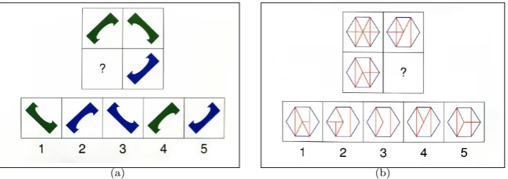
Figure 1: Two examples tasks from the WASI test suite. For each task, users were asked to select which of the five options (1-5) should be placed at the ques-tion mark in the stimuli, such that the rows and columns of this had matching correspondence. (a) A simple example where 3 would be the correct response. (b) A more challenging example: in this case 3 would also be the correct re-sponse.
As a complex cognitive task, visual decision making involves (but not limited to) scanning visual scenes, pattern recognition, identifying targets, discriminat-ing and in some cases detectdiscriminat-ing missdiscriminat-ing information. The matrix reasondiscriminat-ing sub-test of the Wechsler Abbreviated Scale of Intelligence (WASI) is a well known psychological tool that is designed to simulate these different aspects [27]. Two example tasks are shown in Figure 1. The WASI tests have the additional ben-efit that, by design, they avoid the “learning effect” - where response times and behaviour changes as users become attuned to the use of an new interface or tool.
As tasks such as matrix reasoning become progressively more difficult in high pressure settings such as healthcare screening or production quality con-trol individuals’ confidence levels can be impacted. Ais et al. have studied the the factors underlying individual consistency in confidence judgements over four tasks (one auditory, three visual), repeated over a period of time. They concluded that the pattern of judgements across tasks represents a “subjective fingerprint” that can be used to identify subjects [2]. We would speculate that in turn changes in these patterns may be useful to denote changes in cognitive processing.
3
User Confidence Data Collection
5 males and 18 females were recruited to participate in the study, all under-graduate students on a Psychology degree at University of the West of England. Participants viewed the screen from a distance of 60cm. Eye movements were monitored using an Applied Systems Laboratory (ASL) EYE-TRAC D6 running at 60Hz and the ASL Eye-Trac 6 User Interface Program.
3.1
Protocol
Each person was shown a calibration screen and then asked to complete the same sequence of 28 matrix reasoning tasks: sets of individual coloured images composed of geometric designs or patterns where one section or piece is missing. Participants must use reasoning to determine what information is missing and select the appropriate piece from a set of choices. The tasks ranged in difficulty, with the least complex being shown early in the study, progressing through to the most complex. After each task, the participants were shown a screen asking them to respond to the statement “I am confident about my answer”. Users could select their response on a 5-point Likert scale, ranging from 1 (strongly disagree), through 3 (neutral), to 5 (strongly agree).
The data collected was analysed using the ASL Results Standard 2.4.3 Soft-ware. After removing cases where the system was unable to infer gaze, 583 subject-task cases remained, distributed by confidence labels 1–5 as {62, 77, 110, 171, 163}. The raw data for each case consists of a time-stamped sequence of gaze fixations that correspond to x, y coordinates on the screen, where a fixation is defined as a period of at least 100 msec during which the point of regard does not change by more than a 1◦ visual angle. Each fixation was also labeled using the known bounding box of the particular region of interest (ROI) that the fixation point is within, which can either be one of the options that the user can answer with (‘Op[1-5]’), one of the stimuli items currently shown (‘Stim[1-4]’), or outside of these areas of interest (‘outside’).
3.2
Data Characteristics
It is important to understand whether the data has any particular attributes that may influence the ability to predict user confidence. Here, we present a preliminary exploration of its characteristics to understand the problem domain further.
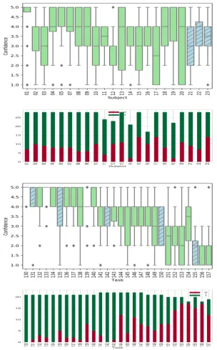
Figure 2 shows the variation in reported confidence, grouped by user and by task. It can be seen that there is considerable variation in the range of values used by different users, and very few make use of the full confidence reporting range of 1-5. When considering the reported confidence by task, it can be seen that confidence decreases for the later tasks (since the tasks get progressively more difficult).
not all subjects completed all tasks. This observation partially motivated our creation of the “Tendency” feature (see below).
Considering the proportions of correct/incorrect responses grouped by tasks, there is a clear pattern that high confidence tends to be associated with tasks which most subjects got right. Correspondingly low reported confidence corre-sponds to low correctness. This partially motivated creation of the “Easiness” feature (see below).
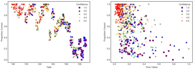
[image:10.595.137.450.400.511.2]The scatter plots in Figure 3 show the relationship between the proportion of correct responses for a task (shown on the y-axis), plotted against the task ID (left), and the time taken to respond (right). For the sake of clarity, a small amount of jittering (random noise) has been applied. The markers signify the reported confidence values. It can be seen that the proportion of users selecting the correct response for a task decreases with task ID, since again, the tasks become progressively more difficult. Considering the relationship between user response time and correctness, it can be seen that there is more variation for the harder problems, and response times tend to be quicker for easier tasks. However, there is a large overlap between successive confidence values, so the response time is not sufficient to clearly separate the 5 classes. Note also, that users tend to report higher confidence in decisions they make quickly, but there is more variation for lower confidence: sometimes users are “sure that they are not sure”.
Figure 3: Scatter plots of relationship between proportion of correct responses and task id (left), and time taken (right). Colours and styles of markers distin-guish levels of reported confidence. Jittering has been applied to aid visualisa-tion.
account of confidence. Thus when dividing by task, the first split comprises the users’ responses for tasks 1–6, the second tasks 7–12 and so on. The third approach (‘Stratified-CV’) attempts to ensure each partition contains a repre-sentative set of confidence values. This assigns cases to splits in rotation - so that again using the example of dividing according to task, the first split com-prises the users’ responses for tasks 1,6,11 etc. We discuss this issue further in Section 5.
4
Prediction Architecture and Methodology
Having collected data from the WASI study, here we describe how we use it to predict the confidence values reported by individual users. Typical machine learning approaches would engineer a collection of representative “summary” features that characterise the user activity, and then train a prediction model to map input features to an output which could be either a categorical class (e.g., confident or not confident), or a continuous value that represents the confidence scale (i.e., in the range 1 –5).
Summary features might include information about where, for how long, and in what sequence, fixations took place. In this study for example, calculating these might include dividing fixations according to whether they were on stim-ulus or options, or neither. This process of mapping from an{x, y}coordinate system onto a set of labelled regions is of course highly problem-specific, and time consuming. Recently there have been significant advances in deep learn-ing for automatlearn-ing this process of feature design and extraction, most notably using Convolutional Neural Networks (CNNs) for image-based tasks. Here the learning algorithms take images, rather than numerical features as inputs, and the first few convolutional layers effectively automate the process of feature engineering.
We next describe a flexible architecture that enables us to combine these approaches, before going on to describe in more detail the process of creating summary features, and the “gazemap” images used by the CNNs. The archi-tecture is designed to allow us to investigate a number of questions such as:
R1: Given the different ranges of confidence values used by subjects, is it better to make categorical or ordinal predictions?
R2: What is the effect of incorporating different levels of domain knowledge in the gazemaps used by the CNNs, or the numerical features?
R3: Can the automated learning process of CNNs create predictors that are
competitive with those using hand-engineered summary statistics? R4: Can the automated learning process of CNNs create predictors that are
complementary to those using hand-engineered summary statistics, in a way that can be exploited to further increase predictive accuracy?
4.1
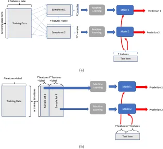
Hybrid Predictive Ensemble Architecture
respec-(a)
[image:12.595.128.465.131.439.2](b)
Figure 4: Architectures for ensemble predictors. Blue lines show process of model induction and red lines show process of predicting value for a new test item. (a): Conventional - each model is trained from a different subset of training items but “sees” all of the features for each training or test item. (b): Hybrid - each model is trained from adisjoint subset of features but ‘’sees” the entire training set.
each model. These can be used individually or combined via a stacking meta-learner, in which case we feed the predictions, (and associated probabilities) into a further prediction algorithm.
4.2
Generating Summary Statistics Features
Many different features can be derived from the raw eye tracking and timing data. Whilst many of these features are quite standard, such as mean values, durations, and counts, they required extensive application-specific processing to calculate, since it is necessary to know, for example, the on-screen regions corresponding to different stimuli and responses for each of the individual tasks. In Appendix A, we present box plots that show the distribution of the values observed for each summary variable as a function of the reported confidence. From observation of these plots, it can be seen that in fact no single feature can provide strong predictive value for classifying participant confidence. In addition, we also use three contextual features that we describe as easiness,
tendency, and mojo. These are derived from the observation data to provide a deeper context for prediction, making use of prior task and user data that is available to inform the current observation. Preliminary results suggests these significantly increase accuracy. Clearly, the suitability of such features in other systems would be application-dependent. Below we describe the contextual features in more detail:
• Theeasiness of the task is measured based on the proportion of correct responses versus incorrect responses, for all participants. This feature was designed to be useful for scenarios where we were interested in monitoring different users on a set of standard tasks for which we had the results from other users. This feature was removed from the data set when predicting the behaviour of known users on new tasks, due to the dependency of knowing about the task.
• Thetendency is a long term measure that is designed to characterise how each user reports their confidence. Currently it only applies to the binary classification case. We calculate this as (RC+W U−RU−W C)/(RC+
RU+W C+W U) where Rindicates a correct response, W indicates an incorrect response, C indicates a confident response (class 4 or 5), and
U indicates an unconfident response. This measure would be particularly useful where a user is expected to interact with a system repeatedly over time. For our case, we calculate this incrementally for each test case, such that it incorporates a notion of ‘familiarity’ with the given task. This feature was removed from the data set when predicting the behaviour of known tasks on new users, due to the dependency of knowing about the user.
feature is used in both predictive cases, since it is computed in real-time as the participant responds to the series of tests, and does not rely on prior knowledge of either the task or the user.
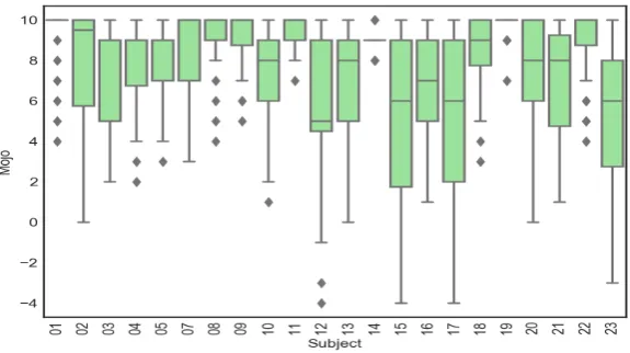
Figure 5: Box-plots of Mojo scores for different users as a means of analysing self-efficacy. Users that have a larger range will have reported that they are uncofident more frequently during the study.
After some initial experimentation, the following summary features were used:
• Time Taken,
• mean duration of fixations on each ROI (Op[1-5], Stim[1-4], and ‘outside’)
• mean pupil dilation during fixations on each ROI (Op[1-5], Stim[1-4], and ‘outside’)
• mean distance between successive fixations
• count of stimuli fixations
• count of option fixations
• count of ‘horizontal’ movements (i.e., stimulus–stimulus or option–option)
• count of ‘vertical’ movements (stimulus-option or option-stimulus)
• time taken to make a decision
• a measure ofeasiness for the task • a measure of user overalltendency
We also present results using a “reduced” feature set of summary features that do not depend on mapping fixation locations onto regions in the specific visual tasks. This reduced feature set is comprised of Time Taken, Tendency, Easiness, Mojo, Number of Fixations, Mean Fix Duration, Mean Pupil Diameter during fixations, and the Mean Distance between fixations.
4.3
Generating Gazemap Image Representations of Eye
Tracking Activity
In conjunction to the traditional summary features that can be used, we also investigate how gazemap image representations could be developed and used for the purpose of predicting user confidence. The concept of a gazemap seems reasonable to represent eye tracking activity due to the inherent nature of the spatial domain when the user is observing the task. Moreover, this approach can potentially save on the need for labourious ‘hand-crafting’ of numerical features to characterise the problem domain, as done in the previous section. In this sense, we can depict the spatial activity as an image and allow the classifier to identify whether there are distinguishing features that can support the separability of the output classes. In this section, we describe our systematic and incremental design scheme for developing gazemaps. We also examine the gazemap image representations in relation to reported confidence values, to assess the potential of being able to classify confidence from such images.
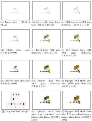
Given that there are many different visual channels that can be used to represent data, such as size, shape, colour, opacity, connection, and orientation, there is a question ofhow should a gazemap image representation be developed? Figure 6 presents the incremental design approach that we adopted for devel-oping different gazemap representations. Intuitively, eye movement data can be considered as a time-series of x, y coordinates, and so we begin by represent-ing this data with connected line segments. The line width can be mapped to the interfix duration time, where a longer duration between fixation points will result in a thicker line. Horizontal movements are shown by a blue line, and vertical movements are shown by a yellow line. The top row shows an initial design scheme to illustrate this. The scheme is extended to also incorporate fixation duration time, shown by the green circles (b). We made use of a popu-lar online colour palette generator,Colorsupplyyy2to select four complimentary colour hues in our designs using the square configuration from the colour wheel (#30499B, #EE4035, #F0A32F, #56B949). In (c), we make use of the region of interest (ROI) information that is collected by the eye tracking tool, to know whether the fixation point is a stimuli item, an option item, or outside either of these ROIs. Gaze movements from option to stimuli are coloured as blue. Gaze movements from stimuli to option are coloured as yellow. Gaze movements be-tween stimuli items or bebe-tween option items are coloured as red. Gaze duration are shown in green, where squares represent fixations on stimuli, and circles rep-resent fixations on options. Each row of Figure 6 follows a similar progression, where the second row increases the original thickness of the gaze lines. This is to increase the amount of information that the convolutional neural network can ‘see’ in the image, since the white background will not be informative. The third row removes alpha to make the image opaque. Initially, it was felt that the
(a) Lines only. (44.62± 30.52)
(b) Lines with gaze dura-tion. (62.53±28.36)
(c) ROI lines with ROI gaze duration. (48.58±31.53)
(d) Thick lines only.
(55.43±30.09)
(e) Thick lines with gaze duration. (78.90±4.46)
(f) ROI thick lines with
ROI gaze duration.
(78.35±5.30)
(g) Opaque thick lines only. (68.63±19.60)
(h) Opaque thick lines
with gaze duration.
(79.83±2.24)
(i) Opaque ROI thick lines with ROI gaze duration. (80.50±4.85)
(j) Original Task Image (k) Opaque thick lines
with gaze duration and shape edge lines. (78.29± 5.21)
[image:16.595.141.453.121.530.2](l) Opaque ROI thick lines with ROI gaze duration and shape edges lines. (80.97± 3.96)
Figure 6: Example gaze map images. We adopt an incremental design strategy for illustrating the influence of gaze map features. Left-to-right, features are in-troduced to incorporate fixation duration markers, and stimuli-option markers. Top-to-bottom, lines are thickened, made opaque, and then shapes are given an outline. Values shown in brackets are mean accuracy and standard deviation for 5-CV on each design scheme.
384×256 pixels.
4.4
Comparison of Gazemap Representations for
Confi-dent and UnconfiConfi-dent Users
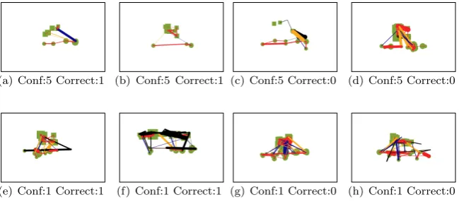
For any predictive classifier to be robust, there need to be some observable characteristics that enable it to identify a particular instance as one class over another, much as if a human was performing the same task. This is well under-stood for image classification tasks. For example, for a classifier that is trained to recognise digits, observing a vertical line may suggest that the digit is a ‘1’, whereas observing a circular area may suggest either a ‘0’ or an ‘8’. Here, we examine a subset of gazemap images, to explore how a system may recognise characteristics suggestive of confident or not confident.
(a) Conf:5 Correct:1 (b) Conf:5 Correct:1 (c) Conf:5 Correct:0 (d) Conf:5 Correct:0
[image:17.595.135.460.292.435.2](e) Conf:1 Correct:1 (f) Conf:1 Correct:1 (g) Conf:1 Correct:0 (h) Conf:1 Correct:0
Figure 7: Example gaze images for different participants to show cases of con-fident and unconcon-fident gazemaps. (a) and (b) are cases where participants are confident and correct, (c) and (d) where participants are confident and incor-rect. (e) and (f) are cases where participants are unconfident and correct, (g) and (h) where participants are unconfident and incorrect.
Figure 7 shows example gazemaps for different participants, to show cases of self-reported confidence (top row) and unconfidence (bottom row). We also include whether the participant’s response was correct (columns 1 and 2) or incorrect (columns 3 and 4). We do not currently account for correctness in our prediction, however there is much scope to pursue this in future research, in particular, investigating whether there a difference between confident users who are correct or incorrect, and likewise those who are unconfident but correct, or unconfident and incorrect? For now however, we primarily study only the difference between the confident and unconfident cases. The samples shown were randomly selected from the pool of available images. On observing these images, it appears that repeated gaze movements back and forth between stimuli and option may suggest unconfidence. This would seem a reasonable judgement for such tasks, where those who are confident may not need to study the task for as long. The confident cases have many fewer fixations, and these appear to have shorter duration.
the separability between confident and unconfident cases. To some extent, the purpose of the CNN is to alleviate the need for examining and identifying what the discriminating variables are between confident and unconfident examples by hand, since the machine can compute many more image feature derivatives that may yield greater separability between the classes, beyond those a human can verbally express. Here, we have begun to demonstrate that there are visual characteristics that could be informative for identifying the separability between confident and unconfident users, which therefore gives justification for adopting image classification techniques for solving this problem. The use of machine learning techniques to better investigate and understand the separability be-tween classes remains an active research area.
4.5
Implementation
The system was implemented in Python, using thescikit-learnlibrary imple-mentations of the machine learning algorithms, and theTensorflowlibrary [1] for the convolutional neural network, accessed via theKeraslibrary [8] to pro-vide a common interface to all the machine learning algorithms. To reduce the likelihood of results being skewed by poor design choices, we used the parameter grid search function (GridSearchCV) fromscikit-learnwith 5-fold cross vali-dation (5-CV). This process randomly divides the training set taking no account of the users or the tasks, and so the mean and standard deviation of the 5-CV results provides an indication of the amount of variability present, and whether the results on the test sets are representative.
Typical image classification tasks rely on hundreds, often even thousands, of possible training samples in order to generalise well to new observations. Given the limited number of participants and tasks that were used in this study, we therefore make use of Keras’ data augmentation routineimageDataGenerator.flow(). This is designed specifically to generate additional training image samples, by replicating examples from the training set and applying small variations to pa-rameters such as translation, rotation, and flip, whilst preserving the original training label. We allowed for translation shifts in bothx ory directions of up to 5% the image size. We also allow for ‘horizontal flips’ – reflections about the midpoint of the x-axis. For each epoch, we create one distorted version of each original training image.
A wide range of different machine learning algorithms from thescikit-learn
library were trialled on the summary features, and where available, classifica-tion and regression methods were tested. In the interest of brevity, we report only the four most successful techniques: Random Forests (RF), Gradient Boost (GB), Support Vector Machines (SV) and Multi-Layer Perceptron (MLP). De-tails of the parameters considered in the grid search for each algorithm, and of the CNN, are given in Appendix B.
4.6
Comparison Metrics
As described in Section 3.2, we consider three ways of generating train/test splits to estimate predictors’ performance. The two cross-validation approaches allow us to report both means and standard deviations for the reported metrics. For the 2-class classification task we removed images which were labelled as “neutral”, and merged the rest into two classes with confidence 0 (original labels “strongly disagree” and “disagree”) and 1 (original labels “agree” and “strongly agree”). This gives a 410:72 split between confident and unconfident. We left the test set unchanged. For the regression problem we used the full 500:83 train/test split.
The metrics chosen for comparison were the binary accuracy for classifi-cation, and the mean absolute and squared error for regression. To permit a comparison between the two approaches, we also report the numbers of False Positive and False Negative predictions. For the classification tasks these have the obvious standard definition. For the regression version, we say that a test case is incorrectly classified when the prediction lies on the ‘wrong side’ of neu-tral. Thus, as a False Positive when the user’s reported confidence for that case was 1 or 2, but the predicted value was>= 3.5 (and hence would be rounded to class 4 or 5). Correspondingly, a prediction of less than 2.5 is judged to be a False Negative when the user’s reported confidence is 4 or 5.
5
Predicting the Confidence of New Users on
Known Tasks
This scenario is predicting the confidence of new users on known tasks. We omit thetendency feature, since there should not be prior knowledge about the tendency of the user in how they report their confidence. The mojo variable is used since this is generated as the participant proceeds through the series of known tasks. Likewise, theeasiness variable can also be used, since the task is already known. None of this information is available in the gazemaps.
5.1
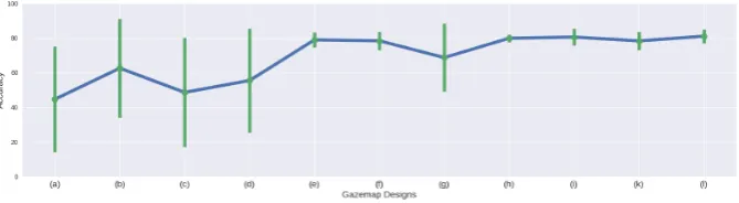
Choice of Gazemaps
As part of our experimentation, we trialled each of the design schemes in Figure 6 with the CNN predictive model to assess their performance. Figure 8 shows the mean accuracy, with standard deviation shown by the error bars on the task of predicting the confidence reported by new users on known tasks as a classification problem, using 5-fold cross validation (5-CV). The labels (a – i) correspond to the labels in Figure 6.
From these results, design scheme (l) (Opaque ROI thick lines with ROI gaze duration and shape edge lines) performs best with an accuracy result of 80.97±3.96. In fact, schemes (e), (f), (h), (i), (k) and (l) all achieve a mean accuracy of over 78%, with standard deviations that suggest no statistically sig-nificant difference in performance. Other methods all show much larger standard deviations, suggesting that the cross-validation splits may have significantly var-ied results. Of particular note is that schemes (e) and (h) achieve good accuracy and yet only make use of fixation duration time, interfix duration time, and the
Figure 8: Mean accuracy and standard deviation results, for each of the visual design schemes (a)-(l) shown in Figure 6. (l) achieves the highest score of 80.97±3.96. Schemes (e), (f), (h), (i), and (k) all score above 78%.
gaze duration) performs best with an accuracy of 79.83±2.24. Importantly, these schemes do not incorporate any task-specific information (unlike (f), (i), (k), and (l)). This is particularly encouraging as it demonstrates that there may be potential to extend this approach for more generalisable applications in the future, rather than relying on domain-specific knowledge. For further testing, we choose to use design schemes (h) and (l), since (h) achieves the greatest accuracy with no task-specific features, whilst (l) achieves the greatest accuracy overall.
5.2
Results for Predicting Confidence as a 2-Class
Classi-fication
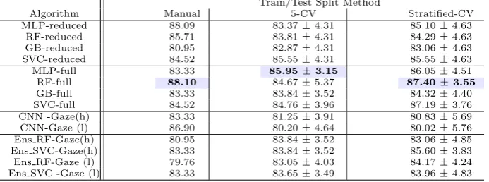
Table 1 shows the prediction results for the 2-class classification task, using the summary features, the gaze images, and the ensemble approach of both combined. We show results for the manually curated train/test split, 5-CV, and stratified cross-validation. For each split method, we highlight the most accurate result in bold.
These results illustrate the large variability between cross-validation splits, and also large variability in the traditional ML approaches versus the CNN techniques. Looking at the manual set, the range of results for the traditional ML approaches vary between 80.95% to 88.10%, whilst the CNN results range from 83.33% to 86.90%, and the ensemble results range from 79.76% to 83.33%. Whilst the MLP-full and RF-full methods show the greatest accuracy, the ac-curacy range from the CNN results and from the ensemble results are both comparatively similar, with the CNN-Gaze (l) achieving greater accuracy than 6 of the other traditional ML experiments.
Comparing equivalent results from full-vs- reduced feature sets, the former always gives higher accuracy, but the differences are not statistically significant taken classifier-by-classifier. Looking at the effect of including task-specific in-formation (l) or not (h) into gazemaps, the effect is to increase accuracy for the manual split, and to reduce it slightly (but not statistically significantly) for the cross-validation metrics.
the errors made by different algorithms are correlated.
Table 1: Mean and standard deviation (where appropriate) of accuracy for classification of confidence of new users on known tasks for different feature sets and classifiers. Ensemble results are suffixed by meta-learner, and where appropriate, the gaze map design scheme is indicated in brackets.
Train/Test Split Method
Algorithm Manual 5-CV Stratified-CV
MLP-reduced 88.09 83.37±4.31 85.10±4.63
RF-reduced 85.71 83.81±4.31 84.29±4.63
GB-reduced 80.95 82.87±4.31 83.06±4.63
SVC-reduced 84.52 85.55±4.31 85.55±4.63
MLP-full 83.33 85.95±3.15 86.05±4.51
RF-full 88.10 84.67±5.37 87.40±3.55
GB-full 83.33 83.84±3.52 84.32±4.40
SVC-full 84.52 84.76±3.96 87.19±3.76
CNN -Gaze(h) 83.33 81.25±3.91 80.83±5.69
CNN-Gaze (l) 86.90 80.20±4.64 80.02±5.76
Ens RF-Gaze(h) 80.95 83.84±3.52 83.06±4.85
Ens SVC-Gaze(h) 83.33 83.84±3.52 85.60±3.83
Ens RF-Gaze (l) 79.76 83.05±4.03 84.17±4.24
Ens SVC -Gaze (l) 83.33 83.65±3.49 83.96±4.83
5.3
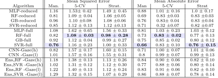
Results for Predicting Confidence as a Continuous
Value
Table 2 shows the results when treating the problem as a regression task to predict confidence as a continuous value. As before, we show the splits for manually-curated, 5-CV, and stratified-CV, and for each we highlight the case where the lowest error is obtained. In a number of the experiments, the predicted value is observed to be less than 1.0 from the actual value. This is particularly encouraging as it suggests that we can make far more nuanced predictions about different levels of confidence.
In almost every case the accuracy observed with the reduced feature set is worse than the corresponding result with the full feature set. However, compar-ing the two sets of CNN results show that includcompar-ing task specific information is unnecessary, making scheme (h) particularly appealing as a generalisable ap-proach for other domains.
For the manually-curated set, the SVR achieves the lowest MSE and MAE. The second lowest MAE is obtained by the CNN-Gaze (h) method, whilst the second lowest MSE is obtained by both CNN-Gaze (h) and RF. Again, this sug-gests that the CNN methods can provide comparable results to the traditional ML techniques. Also again the ensemble approaches do not significantly reduce errors over the baseline methods.
Table 2: Mean and standard deviation (where appropriate) of regression predic-tion accuracy metrics for new users on known tasks, for different algorithms and methods for training/test splits. Ensemble results are suffixed by meta-learner, and where appropriate, the gaze map design scheme is indicated in brackets.
Mean Squared Error Mean Absolute Error
Algorithm Man. 5-CV Strat. Man 5-CV Strat
MLP-reduced 1.16 1.53±0.42 1.49±0.45 0.88 1.01±0.16 1.0±0.17 RF-reduced 0.81 1.09±0.04 1.06±0.05 0.69 0.83±0.03 0.83±0.03 GB-reduced 0.96 1.10±0.08 1.08±0.06 0.76 0.83±0.04 0.83±0.04 SVR-reduced 0.85 1.12±0.13 1.12±0.13 0.71 0.32±0.07 0.82±0.07 MLP-full 1.08 1.62±0.65 1.56±0.33 0.81 1.03±0.23 1.03±0.12 RF-full 0.82 1.08±0.03 0.98±0.28 0.73 0.83±0.02 0.77±0.13 GB-full 0.92 1.12±0.04 0.99±0.27 0.75 0.85±0.02 0.80±0.12 SVR-full 0.76 1.16±0.23 1.00±0.33 0.66 0.83±0.10 0.76±0.15
CNN-Gaze(h) 0.82 1.57±0.17 1.60±0.15 0.71 1.00±0.07 1.01±0.06 CNN -Gaze(l) 1.01 1.57±0.16 1.55±0.31 0.8 0.99±0.07 0.99±0.13 Ens RF -Gaze(h) 1.18 1.38±0.13 1.13±0.26 0.84 0.90±0.06 0.82±0.10 Ens SVR -Gaze(h) 1.02 1.31±0.12 1.12±0.30 0.77 0.88±0.06 0.80±0.14 Ens RF -Gaze(l) 1.22 1.40±0.13 1.12±0.24 0.83 0.91±0.06 0.82±0.10 Ens SVR -Gaze(l) 1.29 1.32±0.15 1.07±0.29 0.86 0.88±0.07 0.78±0.14
for 93%, 87%, and 92% respectively of the variability in the observations – in other words the models are a very good fit in almost every case.
We can observe that the distribution of predictions for each reported con-fidence class is not uniform across the methods. Most notably, the ensemble predictor makes a greater range of predictions, whereas the CNN, and to lesser extent Random Forest tends not to predict low values of confidence. Despite the appearance of outliers in all plots, the R-squared statistic shows that there are a high number of points that do actual fit the ideal line, however due to occlusion in the plot these are not as visually distinct as the outliers. These out-liers, coupled with the use of least-squares fitting, are also the reason why the second, “best-fit” regression lines (dotted) (obtained using the default settings) have a high positive intercepts and a much lower R2 values.
5.4
Comparison of Errors from Classification and
Regres-sion Approaches
(a) (b) (c)
Figure 9: Scatter plots with “Ideal” (dashed) and ”best” (dotted) linear regres-sion lines for results from RF, CNN and Ensemble predictors of the confidences of new users. Predicted values are on the y-axis and the actual values on the x-axis. x-values have a small amount of random noise (jitter) added to aid visualisation.
that there is certainly no clear traditional approach that performs significantly better, and that the CNN methods can perform just as well under a variety of different testing scenarios.
Table 3: Mean and standard deviation (where appropriate) of number of False Positive and False Negative predictions for the confidence of new users on known tasks for different feature sets and contrasting prediction by classification or re-gression. Ensemble results are suffixed by meta-learner, and where appropriate, the gaze map design scheme is indicated in brackets. Highlighting indicates the lowest results in each column
Train/Test Split Method
Classification Regression
Algorithm Man. 5-CV Strat.-CV Man. 5-CV Strat.-CV
False Positive
MLP-full 8 8.4±5.20 10.6±5.40 0 2.2±1.3 2.2±0.80
RF-full 5 10.8±7.30 10.0±5.00 2 4.2±2.9 4.0±2.10 GB-full 9 9.8±5.70 13.0±6.20 3 4.60±2.6 4.0±2.00 SVC-full 6 10.8±6.00 10.4±4.70 2 6.0±4.9 5.8±3.5 CNN-Gaze (h) 6 13.0±6.20 13.6±6.20 2 5.0±4.2 5.6±4.9 CNN-Gaze (l) 7 12.4±6.70 13.6±6.30 2 6.0±3.2 7.6±5.9 Ens RF-Gaze (h) 9 9.6±5.39 11.2±4.87 3 5.0±2.9 5.0±2.6 Ens SVC-Gaze (h) 9 9.8±5.67 11.2±3.97 3 4.8±2.7 5.8±3.6 Ens RF-Gaze (l) 10 9.6±5.39 10.0±4.56 4 6.8±4.3 4.4±1.6 Ens SVC-Gaze (l) 9 9.8±5.67 12.8±5.91 5 6.0±3.2 5.4±2.5
False Negative
MLP-full 6 6.2±3.31 5.4±3.07 10 11.2±7.0 13.0±5.7
RF-full 5 5.0±3.90 4.6±3.01 2 3.2±3.2 2.8±1.7
GB-full 5 7.0±3.29 5.2±3.97 3 2.8±2.7 2.2±1.0
SVC-full 7 5.0±3.52 4.2±2.64 3 2.8±2.8 3.0±1.4
[image:23.595.124.470.504.712.2]6
Predicting the Confidence of Known Users on
New Tasks
In this second scenario, we are interested in predicting the confidence of known users on new tasks. Here we omit theeasiness feature, since there should not be prior knowledge about the difficulty of the new task. We make use of the
tendency feature since we have prior knowledge about how users have reported their confidence previously. As with the previous task, mojo is also used since this is generated on-the-fly as the participant proceeds through the series of tasks. As before, the gazemaps do not contain any of these features.
6.1
Results for Predicting Confidence as a 2-Class
Classi-fication
Table 4 shows the results obtained with different classifiers when predicting the confidence of known users on new tasks. In this case the stratified cross-validation approach is more successful at producing representative splits, with lower standard deviations. When considering the progression of task difficulty, the stratified-CV approach most likely provides a more representative test sam-ple compared to the 5-CV, since it draws test samsam-ples evenly across the full set of tasks, rather than as sequential groupings. Looking at the range of results for the stratified-CV, we see that the traditional ML methods range between 78.26% and 84.97%, the CNN methods range between 78.53% and 79.86% and the ensemble methods range between 82.49% and 84.61%. The CNN results are worse in this experiment, although not statistically significantly so. However, in the case of the manually-curated set, we see that the ensemble methods perform particular well, achieving the joint highest scores with GB, of 87.62%.
[image:24.595.127.469.567.698.2]The full-vs-reduced results are broadly the same for the Manual and 5-CV metrics, but the full feature set gives a 5% increase in accuracy for the Stratified Cross-Validation metric. There was no significant difference in the performance of CNNs using the two different types of gazemaps.
Table 4: Accuracy of predicting confidence of known users on new tasks as a classification problem, for different algorithms and train/test splits. Ensemble results are suffixed by meta-learner, and where appropriate, the gaze map design scheme is indicated in brackets.
Train/Test Split Method
Algorithm Manual 5-CV Stratified-CV
MLP-reduced 84.76 81.81±4.78 79.91±5.29
RF-reduced 81.90 81.43±4.78 79.50±5.29
GB-reduced 85.72 79.34±4.78 78.26±5.29
SVC-reduced 84.76 79.67±4.78 79.67±5.29
MLP-full 83.81 79.89±5.16 84.97±2.90
RF-full 82.86 78.36±5.50 84.40±2.80
GB-full 87.62 75.94±3.77 83.07±3.87
SVC-full 84.76 78.52±7.10 84.77±3.14
CNN-Gaze(h) 74.29 76.94±9.75 79.86±4.75
CNN-Gaze(l) 71.43 75.94±7.64 78.53±3.59
Ens RF-Gaze(h) 84.76 76.51±3.73 82.50±3.91
Ens SVC-Gaze(h) 85.71 75.94±3.77 83.44±3.75
Ens RF-Gaze(l) 87.62 74.64±2.66 82.49±4.35
6.2
Results for Predicting Confidence as a Continuous
Value
[image:25.595.124.482.356.490.2]Table 5 shows the results of applying different regression algorithms to the problem of predicting the confidence of known users on new problems. Again the stratified cross-validation approach shows greater consistency than the simple 5-CV approach, and highlights the differences between full and reduced feature sets. As with the classification variant of this scenario, the CNN results are worse, although not statistically significantly so. In terms of Mean Absolute Error (MAE), we see that the ensemble method with SVR and Gaze (l) has the lowest score for the manually-curated set, whilst the CNN-Gaze (l) methods has the lowest MAE for the 5-CV. The CNN-Gaze (h) method has the lowest MSE result for the 5-CV. Again, despite some cases where the CNN may score slightly lower, this still clearly illustrates how the CNN methods are certainly comparable against their traditional summary feature counterparts.
Table 5: Results of predicting confidence of known users on new tasks as a regression problem. Ensemble results are suffixed by meta-learner, and where appropriate, the gaze map design scheme is indicated in brackets.
Mean Squared Error Mean Absolute Error
Algorithm Man. 5-CV Strat. Man 5-CV Strat
MLP-reduced 1.54 2.48±1.17 2.52±1.15 1.04 1.32±0.38 1.34±0.37 RF-reduced 1.07 1.69±0.40 1.71±0.45 0.78 1.06±0.16 1.07±0.17 GB-reduced 1.02 1.71±0.57 1.70±0.55 0.77 1.08±0.22 1.07±0.22 SVR-reduced 1.07 1.73±0.57 1.73±0.57 0.78 1.06±0.21 1.06±0.21 MLP-full 1.73 2.65±1.07 1.82±0.18 1.09 1.37±0.36 1.12±0.08 RF-full 1.00 1.68±0.31 1.01±0.13 0.76 1.07±0.13 0.79±0.07 GB-full 1.01 1.73±0.37 1.01±0.12 0.77 1.09±0.16 0.78±0.06 SVR-full 1.21 1.66±0.61 0.99±0.08 0.82 1.05±0.23 0.76±0.04
CNN-Gaze(h) 1.80 1.64±0.23 1.42±0.15 1.08 1.04±0.08 0.95±0.07 CNN-Gaze(l) 1.61 1.65±0.41 1.37±0.22 0.96 1.03±0.17 0.94±0.09 Ens RF-Gaze(h) 1.04 2.13±0.50 1.26±0.23 0.74 1.17±0.18 0.85±0.10 Ens SVR-Gaze(h) 1.08 2.18±0.40 1.27±0.22 0.72 1.19±0.14 0.84±0.10 Ens RF-Gaze(l) 1.05 2.08±0.40 1.21±0.25 0.74 1.17±0.16 0.83±0.11 Ens SVR-Gaze(l) 1.05 2.11±0.30 1.26±0.22 0.71 1.17±0.11 0.84±0.09
6.3
Comparison of Errors by Classification and Regression
Table 6 shows the false positives and negative errors observed when using the classification and regression models to predict the confidence of known users on new tasks. It shows results for the different train/testing splits and for each of the different algorithms tested. As seen when predicting the behaviour of new users on known tasks, there are fewer errors when using the regression approach in all but the one case (Multi-Layer Perceptron). We also see a number of cases, such as the manually-curated sets, and the false positives in the stratified-CV classification, where the ensemble methods show the joint lowest error rates. Once again, this suggests that the ensemble methods are performing in line with the more accurate methods, and certainly much better than the less accurate methods.
7
Discussion of Results
Table 6: Mean and standard deviation (where appropriate) of number of False Positive predictions for the confidence of known users on new tasks for different feature sets and algorithms, and contrasting prediction by classification or re-gression. Ensemble results are suffixed by meta-learner, and where appropriate, the gaze map design scheme is indicated in brackets.
Train/Test Split Method
Classification Regression
Algorithm Man. 5-CV Strat.-CV Man. 5-CV Strat.-CV
False Positive
MLP-full 10 9.60±9.16 6.40±2.06 3 2.80±3.66 2.00±1.26
RF-full 12 10.20±9.87 6.80±2.14 5 4.60±6.28 2.20±1.47 GB-full 10 10.60±10.69 7.00±1.26 5 4.00±5.06 2.60±1.50 SVC-full 11 11.60±11.57 6.80±0.98 8 6.60±7.00 2.80±1.83 CNN-Gaze(h) 18 13.40±13.22 9.00±3.03 11 5.80±3.97 5.00±2.28 CNN-Gaze(l) 16 10.00±5.06 10.20±3.06 8 4.20±2.79 4.60±2.15 Ens RF-Gaze(h) 11 7.40±6.97 5.40±2.15 5 5.20±6.05 3.40±1.02 Ens SVC-Gaze(h) 11 10.20±9.93 6.60±1.74 7 5.00±5.66 3.60±1.02 Ens RF-Gaze(l) 10 8.20±8.70 5.20±2.04 5 6.00±6.23 3.00±1.79 Ens SVC-Gaze(l) 10 9.80±9.66 6.00±1.41 5 6.40±7.06 3.00±1.10
False Negative
MLP-full 7 11.40±4.63 9.40±2.42 14 25.80±13.88 15.00±2.61 RF-full 6 12.40±5.00 9.60±1.50 2 8.40±4.41 5.80±2.79 GB-full 3 14.60±7.99 10.80±3.19 2 9.00±4.69 5.80±3.43 SVC-full 5 10.80±6.18 9.20±3.19 2 4.40±3.26 4.60±2.58
CNN-Gaze(h) 9 10.60±7.61 12.20±5.19 6 6.00±1.67 5.40±3.32 CNN-Gaze(l) 14 15.20±10.91 12.40±3.20 6 6.40±2.94 5.40±0.49 Ens RF-Gaze(h) 5 17.20±4.45 13.00±3.29 2 13.20±7.57 7.60±2.58 Ens SVC-Gaze(h) 4 15.00±7.27 10.80±3.19 2 14.20±7.19 7.40±3.07 Ens RF-Gaze(l) 3 18.40±7.36 13.20±3.06 2 12.60±6.18 6.80±3.87 Ens SVC-Gaze(l) 3 16.40±8.87 10.20±3.25 2 14.00±8.07 7.40±3.01
R1: Given the different ranges of confidence values used by subjects, is it better to make categorical or ordinal predictions?
The answer is clearly ordinal. As was seen in Figure 2, many users will report their confidence in different ways. Some will make full use of the 1–5 scale, yet others may (un)intentionally limit themselves to a particular subset. It is difficult to know therefore how comparable between users a particular confidence rating may truly be. This is reflected in the high variability seen when estimating performance by cross-validation, but would be alleviated in deployment when predictors would be trained using the full set of training data. For this reason, we experimented with inducing both binary classification, and ordinal regression, models. Using a measure that labels regression predictions as incorrect if they are on the “wrong side of neutral” (e.g.,a user response of 1 or 2 is predicted as 3.5 or more), Tables 3 and 6 contrast the errors made by the two approaches. They offer conclusive evidence that the regression approach is better able to cope with the variability between subjects. Of course, the other point to note is that for the binary classification we removed the “neutral” images from training and test sets, whereas the regression approach coped well with all cases. In future work, it may be interesting to consider a wider scale, to further study how participants utilise the scale, and whether this can then be used to group similar values together to mitigate subjective opinion of scale meanings.
R2: What is the effect of incorporating different levels of domain knowledge in the gazemaps used by the CNNs, or the numerical features?
rep-resentations that allows us to carefully consider the impact of introducing ad-ditional features from the eye tracking data. We also then describe how the different gazemaps perform in a classification task, shown in Figure 8. It was observed that thicker lines outperform thin lines, suggesting that the CNN can make greater use of thick lines for identifying edges. Since interfix duration is also mapped to line thickness, this essentially results in a larger scaling factor for incorporating this attribute, which may therefore be more distinguishable for the CNN. The introduction of gaze duration shown as circular regions also makes significant improvements to the predictive value of the gazemaps. In com-parison, this increase is much greater than the introduction of region of interest details. This suggests that duration time at gaze fixation points is another key attribute for distinguishing between confident and unconfident observations.
What is particularly interesting is that the schemes that incorporate ROI details (e.g., Gaze (l) - accuracy 80.97±3.96%) are only marginally (and not statistically significantly) better than those that do not (e.g., Gaze (h) - accuracy 79.83±2.24% ). This is particularly important, since it suggests that task-dependent information is not necessarily required. Instead, only the detail of the spatial movement activity, the interfix duration times, and the fixation duration times, are of most predictive value. We would anticipate extending this research with other applications of eye tracking, and being able to assess user confidence. Knowing that the task-independent design schemes can achieve relatively high accuracy results is encouraging for moving towards generalisable application of this approach.
Turning to the numerical summary features, there was evidence that making the full feature set available to the ML algorithms led to more accurate models than just using the reduced feature set. This effect was not statistically signifi-cant when examined for a single metric with a single algorithm. However, given the pattern it may well be that appropriate statistical analysis of the pooled results would reveal the inclusion of task-specific information to be significantly beneficial.
R3: Can the automated learning process of CNNs create predictors that are com-petitive with those using hand-engineered summary statistics?
The answer here is clearly affirmative. The results in Section 5 and Section 6, show that the CNN can learn to predict confidence from gazemaps just as well as traditional machine learning algorithms can learn from summary features. It is worth reminding the reader that the gazemaps do not contain any of the information about users or tasks contained in the mojo, tendency or easiness
features. Given the need to carefully consider which features should and should not be included in traditional approaches, they can often suffer from bias in the inclusion of features - for example the prediction on the “new task” scenario changed dramatically when we removed the “easiness” feature. Whilst we ac-knowledge that there is some argument that gazemap design has to consider what data should be included, as we discussed above, the most important find-ing here is that even a relatively simple representation of eye trackfind-ing activity can yield good predictions of user confidence.
directly represented eye-movements as a gazemap. It was observed that repeated fixations in similar areas can cause issues with occlusion. Of course, this itself is an artefact of trying to capture information about a temporal process in a single image. In future work we intend to investigate the use of recurrent convolutional networks to classify sequences of images - along the lines of successes elsewhere in labelling actions in videos.
R4: Can the automated learning process of CNNs create predictors that are com-plementary to those using hand-engineered summary statistics, in a way that can be exploited by a stacking ensemble algorithm to further increase predictive accuracy?
The answer here is mixed. On one hand, ensemble results in the different scenarios do not exhibit a performance increase over the best single method. So there is no evidence that adding gazemap-CNN based predictors to the pool of “base level” algorithms adds extra diversity. On the other hand, the best-performing algorithm is scenario-dependent, so the meta-learning ensemble ap-proach provides a ‘fail-safe’ method. As an example, when comparing all results, whilst we observe that different techniques may exhibit the best result, we can observe that the Ensemble SVC Gaze (h) method is never the worse result, and so it allows us to establish a lower bound of acceptable result. It may well be that what we observe is simply “outvoting”, since the ensemble meta-learners combine the results from 4 predictors based on summary features and just one using gazemaps. There is scope for further research into ensemble creation.
8
Conclusions
We have demonstrated that we can train machine learning systems to accurately identify users’ confidence as they make decisions about a visual task - based on data from monitoring their eye movements. As a binary confident:unconfident
prediction we attain accuracies of 87-88%, and on a scale of 1–5 we can predict within±0.8 of the users’ reported confidence (MAE). We can attain similar lev-els of accuracy in two complementary scenarios: new users working on known tasks (which would extend to people repeating the same task at intervals), and known users attempting new tasks. We also show results for the numbers of False Positive and Negative predictions, showing that these values are typi-cally extremely low, especially when predicting confidence as an ordinal value (FP/FN in the range 2–5 for 80 test cases).
In future work we aim to investigate the use of metaheuristic search within the space of image mappings to find a gazemap representation that can max-imise the predictive accuracy of the convolutional networks, or the ensemble (these not being necessarily the same). The hypothesis is that although highly computationally expensive, the results will be generalisable - in the sense that a gaze representation that works well (i.e., from which a convolutional network can learn) for these WASI images will also work for other types of visual problems. We also aim to explore further methods of obtaining measures of confidence from users whilst undergoing particular tasks, and to cover a range of different visual tasks, and different user groups.
As discussed originally, the aim is to predict users’ confidence using non-invasive techniques, so as not to disrupt their engagement with the task at hand. As we have demonstrated, there is much potential to achieve this from using eye tracking activity data. There is also considerable scope for extending the work to consider other facets of behaviour such as distraction which are highly relevant to real-world decision making. The rapid pace of development of embedded and wearable devices - such as eye-trackers built in to glasses, and the limited processing power needed to use (rather than train) predictors, suggests that in the relatively near future such systems could be deployed unobtrusively with real benefit for many human-machine interaction systems whether in “smart cars”, healthcare, financial trading, manufacturing or security/military decision making.
References
[1] M. Abadi, A. Agarwal, P. Barham, E. Brevdo, Z. Chen, C. Citro, G.S. Cor-rado, A. Davis, J. Dean, M. Devin, S. Ghemawat, I. Goodfellow, A. Harp, G. Irving, M. Isard, Y. Jia, R. Jozefowicz, L. Kaiser, M. Kudlur, J. Lev-enberg, D. Man´e, R. Monga, S. Moore, D. Murray, C. Olah, M. Schuster, J. Shlens, B. Steiner, I. Sutskever, K. Talwar, P. Tucker, V. Vanhoucke, V. Vasudevan, F. Vi´egas, O. Vinyals, P. Warden, M. Wattenberg, M. Wicke, Y. Yu, and X. Zheng. TensorFlow: Large-scale machine learning on het-erogeneous systems, 2015. Software available from tensorflow.org.
[2] Joaqu´ın Ais, Ariel Zylberberg, Pablo Barttfeld, and Mariano Sigman. In-dividual consistency in the accuracy and distribution of confidence judg-ments. Cognition, 146:377–386, January 2016.
[3] S.Z. Arshad, J. Zhou, C. Bridon, F. Chen, and Y. Wang. Investigating user confidence for uncertainty presentation in predictive decision making. In
Proceedings of the Annual Meeting of the Australian Special Interest Group for Computer Human Interaction, OzCHI ’15, pages 352–360, New York, NY, USA, 2015. ACM.
[4] K. S. Berbaum, E. A. Brandser, E. A. Franken, and D. D. Dorfman. Gaze Dwell Times on Acute Trauma Injuries Missed Because of Satisfaction of Search. Academic radiology, 8(4):304–314, 2001.
[6] P. Caleb-Solly and J.E. Smith. Adaptive Surface Inspection via Interactive Evolution. Image and Vision Computing, 25(7):1058–1072, 2007.
[7] F. Chen. Automatic Multimodal Cognitive Load Measurement (AMCLM). Technical report, National ICT Australia, Sydney, August 2011.
[8] F. Chollet et al. Keras. https://github.com/fchollet/keras, 2015.
[9] J.M. Findlay and I.D. Gilchrist. Active Vision: The Psychology of Looking and Seeing. Oxford University Press, Oxford, 2003.
[10] P. Grimaldi, H. Lau, and M.A. Basso. There are things that we know that we know, and there are things that we do not know we do not know: Confi-dence in decision-making.Neuroscience & Biobehavioral Reviews, 55:88–97, August 2015.
[11] E. Haapalainen, S. Kim, J.F. Forlizzi, and A.K. Dey. Psycho-physiological measures for assessing cognitive load. In Proceedings of the 12th ACM International Conference on Ubiquitous Computing, UbiComp ’10, pages 301–310, New York, NY, USA, 2010. ACM.
[12] I. Jraidi, M. Chaouachi, and C. Frasson. Automatic Detection of User’s Uncertainty in Problem Solving Task: A Multimodal Approach. In Pro-ceedings of the Twenty-Fourth International Florida Artificial Intelligence Research Society Conference, pages 31–36, USA, July 2011. Association for the Advancement of Artificial Intelligence.
[13] I. Jraidi and C. Frasson. Student’s Uncertainty Modeling through a Multimodal Sensor-Based Approach. Educational Technology & Society, 16(1):219–230, 2013.
[14] P.A. Legg, O. Buckley, M. Goldsmith, and S. Creese. Caught in the act of an insider attack: Detection and assessment of insider threat. In IEEE Symposium on Technologies for Homeland Security 2015, pages 1–6, Pis-catway, NJ, 2015. IEEE, IEEE Press.
[15] P.A. Legg, D.H.S. Chung, M.L. Parry, R. Bown, M.W. Jones, I.W. Griffiths, and M. Chen. Transformation of an uncertain video search pipeline to a sketch-based visual analytics loop.IEEE transactions on Visualization and Computer Graphics, 19(12):2109–2118, 2013.
[16] E. Lughofer, J.E. Smith, M.A. Tahir, P. Caleb-Solly, C. Eitzinger, D. San-nen, and M. Nuttin. Human-machine interaction issues in quality control based on on-line image classification. IEEE Transactions on Systems Man and Cybernetics, Part A, 39(5):960–971, 2009.
[17] S.W. McQuiggan, S. Lee, and J.C. Lester. Predicting user physiological response for interactive environments: An inductive approach. In AIIDE, pages 60–65, Stanford, CA, USA, 2006. AAAI Press.
[19] D.K. Peterson and G.F. Pitz. Confidence, uncertainty, and the use of information. Journal of Experimental Psychology: Learning, Memory, and Cognition, 14(1):85–92, 1988.
[20] H. Raghavan, O. Madani, and R. Jones. Active Learning with Feedback on Both Features and Instances. Journal of Machine Learning Research, 7:1655–1686, August 2006.
[21] Thomas Roderer and Claudia M Roebers. Explicit and implicit confidence judgments and developmental differences in metamemory: an eye-tracking approach. Metacognition and Learning, 5(3):229–250, July 2010.
[22] C.L. Simons, J. Smith, and P. White. Interactive ant colony optimization (iACO) for early lifecycle software design. Swarm Intelligence, 8(2):139– 157, June 2014.
[23] Ben Steichen, Cristina Conati, and Giuseppe Carenini. Inferring Visualiza-tion Task Properties, User Performance, and User Cognitive Abilities from Eye Gaze Data. ACM Transactions on Interactive Intelligent Systems, 4(2):1–29, July 2014.
[24] A.L. Thomaz and C. Breazeal. Teachable robots: Understanding human teaching behavior to build more effective robot learners. Artificial Intelli-gence, 172(6-7):716–737, 2008.
[25] C. Umoja, X. Yu, and R. Harrison. Fuzzy and Uncertain Learning Tech-niques for the Analysis and Prediction Of Protein Tertiary Structures, pages 190–211. John Wiley and Sons, Inc, Hoboken, NJ, USA, 2015.
[26] S. Wang and H. Takagi. Improving the Performance of Predicting Users’ Subjective Evaluation Characteristics to Reduce Their Fatigue in IEC.
Journal of physiological anthropology and Applied Human Sciences, 24:81– 85, 2005.