Munich Personal RePEc Archive
Matching Estimators with Few Treated
and Many Control Observations
Ferman, Bruno
Sao Paulo School of Economics - FGV
4 May 2017
Matching Estimators with Few Treated and
Many Control Observations
∗
Bruno Ferman
†Sao Paulo School of Economics - FGV
First Draft: May, 2017
This Draft: September, 2018
Please click here for the most recent version
Abstract
We analyze the properties of matching estimators when there are few treated, but many control observations. We show that, under standard assumptions, the nearest neighbor matching estimator for the average treatment effect on the treated is asymptotically unbiased in this framework. However, when the number of treated observations is fixed, the estimator is not consistent, and it is generally not asymptotically normal. Since standard inferential techniques are inadequate in this setting, we propose alternative inferential procedures based on the theory of randomization tests under approximate symmetry.
Keywords: matching estimators, treatment effects, hypothesis testing, randomization
infer-ence
JEL Codes: C12; C13; C21
∗The author gratefully acknowledges the comments and suggestions of Luis Alvarez, Ricardo Paes de
Barros, Lucas Finamor, Sergio Firpo, Ricardo Masini, Cristine Pinto, Vitor Possebom, Pedro Sant’Anna, and participants of the 2017 California Econometrics Conference and of the Rio-Sao Paulo Econometrics Conference. Deivis Angeli provided outstanding research assistance.
1
Introduction
Matching estimators have been widely used for the estimation of treatment effects
un-der a conditional independence assumption (CIA).1 In many cases, matching estimators
have been applied in settings where (1) the interest is in the average treatment effect for the
treated (ATT), and (2) there is a large reservoir of potential controls (Imbens and Wooldridge
(2009)). Abadie and Imbens(2006) study the asymptotic properties of matching estimators
when the number of control observations grows at a higher rate than the number of treated
observations. However, their asymptotic results still depend on both the number of treated
and control observations going to infinity. Therefore, reliance on such asymptotic
approxi-mations should be considered with caution when the number of treated observations is small,
even if the total number of observations is large.
In this paper, we analyze the properties of matching estimators when the number of
treated observations is fixed, while the number of control observations goes to infinity. We
first show that the nearest neighbor matching estimator is asymptotically unbiased for the
ATT, under standard assumptions used in the literature on estimation of treatment effects
under selection on observables.2 This is consistent with Abadie and Imbens (2006), who
show that the conditional bias of the matching estimator can be ignored, provided that the
number of control observations increases fast enough, relative to the number of treated
ob-servations. In their setting, the matching estimator is consistent and asymptotically normal.
In our setting, however, the variance of the matching estimator does not converge to zero,
and the estimator will not generally be asymptotically normal. Our theoretical results
pro-vide a better approximation to the behavior of the matching estimator relative to Abadie
and Imbens (2006) in settings where there is a larger number of control relative to treated
observations, but the number of treated observations is not large enough, so that we cannot
1SeeImbens(2004),Imbens and Wooldridge(2009), andImbens(2014) for reviews.
2This is true whether we consider the average treatment effect on the treated conditional or unconditional
rely on asymptotic results that assume that the number of treated observations goes to
in-finity.3 We conduct an empirical Monte Carlo (MC) study based on real data, as suggested
by Huber et al. (2013). When the dimensionality of the covariates is low, and we consider
matching estimators with few nearest neighbors, our simulations suggest that, regardless of
the number of treated observations, the bias of the matching estimator is close to zero, even
when the number of control observations is not large. Increasing the dimensionality of the
covariates and/or increasing the number of nearest neighbors used in the estimation implies
that we need an increasing number of controls to keep our approximations reliable.
The fact that the matching estimator is not asymptotically normal, in our setting, poses
important challenges when it comes to inference. Inference based on the asymptotic
distri-bution of the matching estimator derived by Abadie and Imbens(2006) should not provide
a good approximation when the number of treated observations is very small, even if there
are many control observations. The bootstrap procedure proposed by Otsu and Rai (2017)
also relies on the number of both treated and control observations going to infinity. For
finite samples, Rosenbaum (1984) and Rosenbaum (2002) consider permutation tests for
observational studies under strong ignorability. However, these tests rely on restrictive
as-sumptions.4 Rothe (2017) provides robust confidence intervals for average treatment effects
under limited overlap. For the case with continuous covariates, he combines his method with
subclassification on the propensity score. However, with few treated observations, it would
not be possible to reliably estimate a propensity score. Therefore, we consider two
alter-native inference methods based on the theory of randomization tests under an approximate
symmetry assumption, developed by Canay et al. (2017). One test relies on permutations,
while the other relies on group transformations given by sign changes.5 We derive conditions
3The finite sample properties of matching and other related estimators have been evaluated in detail in
simulations by, for example,Frolich(2004),Busso et al.(2014),Huber et al.(2013), andBodory et al.(2018). In contrast to their approach, we provide theoretical and simulation results holding the number of treated observations fixed, but relying on the number of control observations going to infinity.
4
Rosenbaum (1984) assumes that the propensity score follows a logit model, while Rosenbaum (2002) assumes that observations are matched in pairs such that the probability of treatment assignment is the same conditional on the pair.
under which these tests provide asymptotically valid hypothesis testing when the number of
control observations goes to infinity, even when the number of treated observations remains
fixed.
The different test procedures we consider present important trade-offs in terms of size
distortion, power, and the underlying null hypothesis they rely on. With few treated
obser-vations, tests based on the asymptotic distribution derived by Abadie and Imbens (2006)
and on the bootstrap procedure proposed by Otsu and Rai (2017) can have important size
distortions, while the two randomization inference tests we propose control well for size even
when the number of treated observations is very small. However, the randomization
infer-ence tests rely on sharper null hypotheses. We show that the size distortion and power for
each test depend crucially on the number of treated observations, the number of control
ob-servations, and the number of nearest neighbors used in the estimation, providing guidance
on how to evaluate the trade-offs among these test procedures in different scenarios.
As an empirical illustration, we consider the “Jovem de Futuro” (Youth of the Future)
program. This is a program that has been running in Brazil since 2008, aimed at improving
the quality of education in public schools by improving management practices and allocating
grants to treated schools. In 2010, this program was implemented in a randomized control
trial with 15 treated schools in Rio de Janeiro and 39 treated schools in Sao Paulo. We
estimate the effects of the program using a matching estimator with the non-experimental
sample as the control schools. We take advantage of the fact that there were about 1,000
other public schools in Rio de Janeiro and more than 3,000 other public schools in Sao Paulo
that did not participate in the experiment, therefore, providing a setting with few treated
and many control observations.6 We find marginally significant treatment effects for Sao
Paulo, and small and insignificant effects for Rio de Janeiro, which is consistent with the
by Canay and Kamat (2018) for regression discontinuity designs, while a test based on sign changes has been studied in the context of an approximate symmetry assumption byCanay et al. (2017) for a series of applications.
6
estimates based on the randomized control trial. Moreover, using the experimental control
schools as the treated group for the matching estimator (so that we should expect to find
no significant results), we provide empirical evidence that inference based on the asymptotic
distribution derived byAbadie and Imbens(2006) may lead to over-rejection when there are
very few treated observations, while the randomization inference procedures control better
for size in this case.
The remainder of this paper proceeds as follows. We present our theoretical setup in
Section 2. In Section 3, we derive the asymptotic distribution of the matching estimator
and derive conditions under which it is asymptotically unbiased. In Section 4, we consider
alternative inference methods that are asymptotically valid when the number of control
observations goes to infinity, while the number of treated observations remains fixed. In
Section5, we present an empirical MC simulation based on the “Jovem de Futuro” program,
and estimate the effects of this program using a matching estimator. In Section6, we contrast
the different inference procedures in light of the theoretical results presented in Section 4
and the simulations presented in Section 5, providing guidance on which method should be
chosen depending on the setting. Concluding remarks, including a discussion of potential
implications for Synthetic Control applications, are presented in Section 7.
2
Setting and Notation
We are interested in estimating the effect of a binary treatment on some outcome.
Fol-lowing Rubin (1973), for each unit iwe denote the potential outcomes Yi(1) if observation i
receives treatment and Yi(0) if observation i does not receive treatment. Therefore, the ob-served outcome for unitiis given byYi =WiYi(1)+(1−Wi)Yi(0), where variableWi ∈ {0,1} indicates the treatment received. In addition to Yi andWi, we also observe for each unit ia continuous random vector of pretreatment variables of dimension k in Rk, which we denote
points, can be easily dealt with by estimating treatment effects within subsamples defined
by their values, and then aggregating on such covariates, as argued by Abadie and Imbens
(2006). We assume that we observe a sample ofN1 treated (N0 control) units that consists of i.i.d. observations of units with Wi = 1 (Wi = 0), and that treated and control observations are independent. Let Iw denote the set of indexes for observations with Wi =w.
Assumption 1 (Sample) For w ∈ {0,1}, {Yi, Xi}i∈Iw consists of Nw i.i.d. observations
with Wi = w. Furthermore, we assume that individuals in the treated and control samples
are independent.
We consider the case in which the number of treated observations (N1) is fixed, while the number of control observations (N0) goes to infinity. One possibility is that there is a large set of units that could potentially be treated, but only a finite number of those units actually
receive treatment. For example, in the empirical application, to be presented in Section 5,
there are a large number of schools that could potentially receive the treatment, but only a
small number of schools actually received it. Alternatively, we can imagine that there are a
large number of treated units, but we only have data from a small sample of them.
We focus on two distinct estimands. First, we consider the conditional average treatment
effect on the treated (CATT):
τ({Xi}i∈I1)≡ 1
N1
X
i∈I1
E[Yi(1)−Yi(0)|Xi, Wi = 1] (1)
which is, conditional on the realization of {Xi}i∈I1, the expected treatment effect for the treated units with these covariate values. We also consider the unconditional average
treat-ment effect on the treated (UATT), which we denote by
τ′ ≡E[Yi(1)−Yi(0)|Wi = 1]. (2)
because, given our setting with N1 finite and N0 large, there is no hope of constructing a counterfactual for the control observations using only a finite set of treated observations.
In the framework of Imbens and Rubin(2015), these two estimands are defined based on a
super-population.
Assumption1does not impose any restriction on how the distribution of (Yi(1), Yi(0), Xi) for treated and control observations may differ. The following assumption does restrict the
way in which these distributions may differ.
Assumption 2 (Conditional Independence Assumption) Conditional onXi, the
dis-tribution of Yi(0) is the same for i in the treated and in the control groups.
Assumption 2 is equivalent to the conditional independence assumption (CIA). While in
Assumption 1 we allow for different distributions of (Yi(0), Yi(1), Xi) whether i is treated or control, Assumption 2 restricts that the conditional distribution of Yi(0) given Xi is the same for both treatment and control observations.7 However, the density of X
i for the
treated observations (f1(Xi)) can potentially be different from the density of Xi for the control observations (f0(Xi)). This is what generates potential bias in a simple comparison of means between treated and control groups, without taking into account that these groups
might have different distributions of covariates Xi.
The next assumption states that possible values of Xi for the treated observations are in the support of the distribution of Xi for the control observations.
Assumption 3 (Overlap) X1 ⊂X0, where Xw is the support of fw(Xi), for w∈ {0,1}
Assumption 3replaces the standard assumption thatP r(W = 1|X =x)<1−ηfor some
η > 0. This assumption guarantees that, for each i in the treated group, we can find an observation j in the control group with covariates Xj arbitrarily close to Xi whenN0 → ∞.
7We do not need to impose such restriction on
Yi(1) because of our focus on average treatment effects on
The main identification problem arises from the fact that we observe eitherYi(1) orYi(0) for each observation i. Note that, if we had two observations, i ∈ I1 and j ∈ I0, with
Xi = Xj = x, then, under Assumption 2, E[Yi|Wi = 1, Xi = x]−E[Yj|Wj = 0, Xj = x] =
E[Yi(1) −Yi(0)|Xi = x, Wi = 1]. The main challenge is that, with a continuous random
variable Xi, the probability of finding observations with exactly the same Xi is zero. The idea of the nearest neighbor matching estimator is to input the missing potential outcomes
of a treated observationi∈ I1 with observations in the control groupj ∈ I0 that are as close as possible in terms of covariates Xi. More specifically, for a given metric d(a, b) in Rk, let
JM(i) be the set of M nearest neighbors in the control group of observation i ∈ I1. Then the matching estimator is given by
ˆ
τ = 1
N1
X
i∈I1
Yi− 1
M
X
j∈JM(i)
Yj
. (3)
3
Asymptotic Unbiasedness and Asymptotic
Distribu-tion
For w ∈ {0,1}, we define µ(x, w) = E[Y|X = x, W = w] and ǫi = Yi − µ(Xi, Wi).
Since we are focusing on the average treatment effect on the treated, we also defineµw(x) =
E[Y(w)|X = x, Wi = 1].8 Under Assumption 2, we have that µ(x,0) = µ0(x). Using this
notation, note that the CATT is given by
τ({Xi}i∈I1) = 1
N1
X
i∈I1
[µ1(Xi)−µ0(Xi)] (4)
8Note that Abadie and Imbens (2006) define
µw(x) = E[Y(w)|X = x]. We use a slightly different
and
ˆ
τ = 1
N1 X i∈I1
µ1(Xi)− 1
M
X
j∈JM(i)
µ0(Xj)
+
ǫi− 1
M
X
j∈JM(i)
ǫj
. (5)
We first show that ˆτ is an asymptotically unbiased estimator for the CATT when the number of treated observations is fixed and the number of control observations grows, and
we derive its asymptotic distribution in this setting.
Proposition 1 Under Assumptions 1, 2, and 3,
1. If µ0(x) is continuous and bounded, then E[ˆτ|{Xi}i∈I1] →τ({Xi}i∈I1) when N0 → ∞
and N1 is fixed.
2. If ˜h(x) = E[h(Y(0))|X = x] is continuous and bounded for any h(y) continuous and
bounded, then, conditional on {Xi}i∈I1,
ˆ
τ →d τ({Xi}i∈I1) + 1
N1
X
i∈I1
ǫi− 1
M
M
X
m=1
ǫm(Xi)
!
whenN0 → ∞ and N1 is fixed
where ǫm(Xi)=d Yi(0)|Xi−µ0(Xi) fori∈ I1, and ǫm(Xi) is independent across m and
i.
Proof. See details in Appendix A.1.1. Let Xi
(m) be the covariate value of the m-closest match to observation i. The main intuition for the results in Proposition1is that, for a fixedXi = ¯x,X(m)i
p
→x¯whenN0 → ∞, because, holdingM fixed, we will always be able to findM observations in the control group that are arbitrarily close to ¯x. Independence ofǫm(Xi) acrossm and i follows from the fact that the probability of two treated observations sharing the same nearest neighbor converges
to zero.
∞. We also derive the asymptotic distribution of the matching estimator conditional on
{Xi}i∈I1, which is centered on τ({Xi}i∈I1). This is important for the construction of the inference methods we propose in Section 4. These results are valid for any fixed value ofN1, including the case withN1 = 1.
Remark 1 The condition that µ0(x) is continuous and bounded would be satisfied if we assume that µ0(x) is continuous and X0 is compact, as is assumed by Abadie and Imbens
(2006). The intuition behind the assumption used in part 2 of Proposition 1is that the
con-ditional distribution ofY(0) given X =xchanges “smoothly” with x. This guarantees that the outcome of the m-closest match to treated observation i, Y(m)i , converges in distribution toYi(0)|Xi = ¯xwhen X(m)i
p
→x¯. In AppendixA.1.2, we show that this condition is satisfied if, for example, Y(0)|X =x∼N(θ(x), σ(x)), where θ(x) and σ(x) are continuous functions of x.
Remark 2 We focus on the properties of the matching estimator conditional on {Xi}i∈I1. We might be interested, however, in the unconditional properties of the matching estimator.
Under the assumptions from part 1 of Proposition 1, E[ˆτ] =E{E[ˆτ|{Xi}i∈I1]} converges to
τ′, which is the UATT. See details in Appendix A.1.3.
Remark 3 With N1 fixed, the estimator is not consistent. This happens because, with a fixed number of treated observations, we cannot apply a law of large numbers to the average
of the error of the treated observations. For the same reason, the matching estimator will not
be asymptotically normal, unless we assume that the error ǫi is normal. These conclusions are similar to the ones derived by Conley and Taber (2011) for differences-in-differences
estimators with few treated groups.
Remark 4 Consider a bias-corrected estimator given by
ˆ
τbiasadj = 1
N1
X
i∈I1
Yi− 1
M
X
j∈JM(i)
(Yj + ˆµ0(Xi)−µˆ0(Xj))
where ˆµ0(Xi) is an estimator forµ0(Xi). With additional assumptions, we can also guarantee that ˆτbiasadj has the same asymptotic distribution as ˆτ. The intuition is that ˆµ0(Xi)−µˆ0(X(m)i ) converges in probability to zero whenN0 → ∞, becauseX(m)i
p
→Xi. See details in Appendix
A.1.4.
Remark 5 We consider an asymptotic framework in whichM is held fixed, whileN0 → ∞, which is similar to whatAbadie and Imbens(2006) call fixed-M asymptotics in their setting.9
As argued byAbadie and Imbens (2006), the motivation for such fixed-M asymptotics is to provide an approximation to the sampling distribution of matching estimators with a small
number of matches. Matching estimators using few matches have been widely used in applied
work (see Abadie and Imbens (2006)). Moreover, Imbens and Rubin (2015) argue against
using matching estimators with many matches, as this would tends to increase the bias of
the resulting estimator, while the marginal gains in precision of increasing the number of
matches are limited.
4
Inference
The fact that the matching estimator is not generally asymptotically normal whenN1 is fixed and N0 → ∞ poses an important challenge when it comes to inference. In particular, inference based on the asymptotically normal distribution derived by Abadie and Imbens
(2006), or on the bootstrap procedure suggested byOtsu and Rai(2017), should not provide
a good approximation in our setting, as the asymptotic theory behind these methods rely
on both N1 and N0 going to infinity. We therefore consider alternative inference methods based on the theory of randomization tests under an approximate symmetry assumption,
developed by Canay et al. (2017). We derive conditions under which these methods are
asymptotically valid when N0 → ∞, even with fixed N1. The first test is based on group transformations given by permutations, while the second test is based on group
transforma-9The difference relative to the framework considered byAbadie and Imbens (2006) is that we also hold
tions given by sign changes. An important caveat is that these different tests differ in their
underlying assumptions and null hypotheses. Moreover, the size and power of these tests
depend crucially on the number of treated and control observations, and also on the number
of nearest neighbors used in the estimation. In Section6, we contrast the different inference
procedures, providing guidance on how to evaluate these trade-offs in different settings.
4.1
Randomization Inference Test Based on Permutations
Consider a function of the data given by
˜
SN0 =
˜
SN0,10 ,S˜N0,11 , ...,S˜N0,1M , ...,S˜N0,N10 ,S˜N01 ,N1, ...,S˜N0M,N1′ (7)
where ˜SN0,i0 =Yi and ˜SN0,im =Y i
(m) for m = 1, ..., M. That is, ˜SN0 is a vector containing the outcomes of the treated observations and of their M-nearest neighbors. The distribution of
˜
SN0 depends on N0, because the quality of the matches will depend on N0. In this notation, the matching estimator is given by
ˆ
τ = 1
N1 N1
X
i=1 ˜
SN00,i− 1 M
M
X
j=1 ˜
SN0,ij
!
. (8)
Let ˜Gi be the set of all permutations πi = (πi(0), ..., πi(M)) of {0,1, ..., M}, π =
⊗N1
i=1πi, and ˜G = ⊗ N1
i=1G˜i. Note that ˜G is the set of all permutations that reassign the treatment status conditional on having exactly one treated observation for each group of
treated observation i and its M nearest neighbors. For a given π ∈ G˜, consider ˜SNπ0 =
˜
SNπ1(0)0,1 ,S˜Nπ1(1)0,1, ...,S˜Nπ1(M)0,1 , ...,S˜πN1(0)
N0,N1 ,S˜ πN1(1)
N0,N1 , ...,S˜ πN1(M)
N0,N1
′
.
Let ˜K =|G˜| and denote by
˜
the ordered values of {T˜( ˜Sπ
N0) :π ∈G˜}, where
˜
T( ˜SN0π ) =
" 1 N1 N1 X i=1 ˜
Sπi(0)
N0,i − 1 M M X j=1 ˜
Sπi(j)
N0,i
!#2
. (10)
We set ˜k = ⌈K˜(1− α)⌉, where α is the significance level of the test, and define the decision rule of the test as
˜
φ(SN0) =
1 if ˜T( ˜SN1)>T˜(˜k)( ˜SN1) 0 if ˜T( ˜SN1)≤T˜(˜k)( ˜SN1).
(11)
In words, we calculate the test statistic ˜T( ˜Sπ
N0) for all possible permutations in ˜G, and then we reject the null if the actual test statistic ˜T( ˜SN0) is large relative to the distribution given by these permutations.
We show that, if we consider the null hypothesis
H0 :Yi(0)|Xi d
=Yi(1)|Xi for all i∈ I1, (12)
then such test is asymptotically levelα, meaning that probability of rejection under the null converges to a value lower or equal to α when N0 → ∞.
Proposition 2 Suppose the assumptions used in part 2 of Proposition 1 are valid, and that the distribution of Yi(0)|Xi is continuous. If we consider the problem of testing 12, then a
test based on the decision rule defined in 11 is asymptotically level α, for any α ∈ (0,1),
when N0 → ∞ and N1 is fixed.
Proof. See details of the proof in Appendix A.1.5.
The main intuition of the proof is that, when N0 → ∞, the limiting distribution of ˜SN0, under the null, is invariant to the transformations in ˜G. From the proof of Proposition
1, note that SNm0,i = Y i (m)
d
that Yi(0)|Xi d
= Yi(1)|Xi, we have that ˜SN0,ij →d Yi(0)|Xi for all j = 0, ..., M. Moreover, asymptotically, ˜SNj0,i is independent across iand j, because the probability that two treated units share the same nearest neighbor converges to zero when N0 → ∞.
Remark 6 Rosenbaum (2002) considers Fisher exact tests in observational studies with matched pairs. He shows that, if the probability of treatment assignment is the same for
both observations in each pair, then a permutation test conditional on the pair is valid, even
in finite samples. With a finiteN0and continuousX, however, it is not possible to guarantee this condition, even under Assumption2, since we will not have, in general, a perfect match
in terms of covariates. We show that this condition can be approximately satisfied when
N0 → ∞ and N1 is fixed using the theory of randomization inference under approximate symmetry developed by Canay et al.(2017).
Remark 7 The null hypothesis12implies thatτ({Xi}i∈I) = 0, but the converse is not true. To understand why this is crucial for this test, suppose, for example, that E[Yi(1)|Xi] = E[Yi(0)|Xi] for all i ∈ I, but V[Yi(1)|Xi] > V[Yi(0)|Xi]. If M > 1, then a permutation
that uses control observations in place of treated ones would have a less volatile distribution
relative to the distribution of the matching estimator. This would lead to a rejection rate
higher than α.10 This is an important drawback of this test, if the underlying interest is in
testing whether τ({Xi}i∈I1) = 0, because the test may reject at a rate higher than α even when τ({Xi}i∈I1) = 0. However, we need to consider a more stringent null hypothesis to guarantee that the test is valid for any fixed value of N1 (even for N1 = 1). Tests that rely on this kind of null hypothesis have received increasing attention, particularly in randomized
experiment settings (e.g. Young(2015)). In Section 4.2 we present an alternative test, that
is also valid with fixed N1, that rely on a less stringent null hypothesis.
Remark 8 This permutation test is similar in spirit to the test proposed by Conley and Taber (2011) for differences-in-differences with few treated and many control groups. Note
10Following the same logic, this also implies that such a test may have a low power if the treatment
decreases the variance of the outcome (that is,V[Yi(1)|Xi]<V[Yi(0)|Xi]). SeeFerman and Pinto(2018) for
that they assume that errors are i.i.d. across groups. In line with their results, the
permu-tation test we propose would also be asymptotically valid if, for example, we test the null
hypothesis τ({Xi}i∈I1) = 0 (instead of the null hypothesis 12), but we impose the assump-tions that ǫi is i.i.d. for alli, and that treatment effect is homogeneous. This highlights the fact that we need to rely on stronger assumptions if we want to construct a test that is valid
regardless of the number of treated observations.11
Remark 9 As outlined by Bugni et al. (2018), the null hypothesis Yi(0)|Xi d
= Yi(1)|Xi is implied by what is sometimes referred to as a “sharp null hypothesis,” in whichYi(1) =Yi(0) with probability one.
Remark 10 The test would remain valid if we consider the null hypothesis Yi(0)|Xi d =
Yi(1)|Xi +ci for all i ∈ I1, for a known vector of constants c = (c1, ..., cN1), instead of the null hypothesis defined in 12.
Remark 11 Canay et al. (2017) consider a randomized version of the test to deal with cases such that ˜T( ˜SN1) =T(˜k)( ˜SN1). Their approach guarantees a test with asymptotic size
α. We focus on the non-randomized version of the test that rejects the null hypothesis if ˜
T( ˜SN1) > T˜ (˜k)( ˜S
N1), which guarantees that the test is asymptotically level α, although it may be conservative. The under rejection will only be relevant if ˜K is very small, where ˜K
is a function of N1 and M.
Remark 12 This test is asymptotically valid, when N0 → ∞, in part because the proba-bility that different treated observations share the same nearest neighbor goes to zero. In
finite samples, however, this may not be the case, and two treated observations will likely
11Ferman and Pinto(2018) consider a method similar to the one proposed byConley and Taber(2011), but that allows for specific forms of heteroskedasticity based on the observed covariates. However, if we consider that all the observable variables that may induce heteroskedasticity are already included as covariates in the matching process, then this would be innocuous. More specifically, in this case, we would already be considering only permutations of observations with similar values ofXi, which is essentially a non-parametric
share the same nearest neighbor when N0 is not large enough relative to N1 and M. To take that into account, we consider a finite sample fix in the permutation test. If a control
observation is the nearest neighbor for two or more treated observations, then we restrict to
permutations of SN0 such that this control observation is always placed as either treated or control. Since the probability that two treated observations share the same nearest neighbor
goes to zero when N1 is fixed and N0 → ∞, for a fixed M, this finite sample adjustment is asymptotically irrelevant.12
Remark 13 This test is also asymptotically valid for bias-corrected matching estimators, as presented in 6. In this case, we define ˜SN00,i=Yi and ˜S
m N0,i=Y
i
(m)+ ˆµ0(Xi)−µˆ0(X i
(m)). The key idea is that, again, ˜Sm
N0,i = Y i
(m)+ ˆµ0(Xi)−µˆ0(X(m)i ) d
→ Yi(0)|Xi, for all m = 1, ..., M, because ˆµ0(Xi)−µˆ0(X(m)i )
p
→0.
4.2
Randomization Inference Test Based on Sign Changes
We consider now an alternative function of the data given by
SN0 = ˆτ1N0, ...,τˆ N0 N1
′
(13)
where ˆτiN0 =Yi−M1 Pj∈JM(i)Yj. Each ˆτiN0 depends on theM nearest neighbors of observation
i, so its distribution depends on N0.
Following Canay et al. (2017), we consider a test statistic given by
T(SN0) = | ˆ
τ|
q
1 N1−1
PN1 i=1(ˆτ
N0 i −ˆτ)2
(14)
where ˆτ = 1 N1
P
i∈I1ˆτ N0
i is the matching estimator for the treatment effects on the treated.
12Another alternative would be to consider a matching estimator without replacement. However, this
We consider the group of transformations given by G = {−1,1}N1, where gS N0 =
g1τˆ1N0, ..., gN1τˆNN10
′
. Let K =|G| and denote by
T(1)(SN0)≤T (2)(S
N0)≤...≤T (K)(S
N0) (15)
the ordered values of {T(gSN0) :g ∈ G}. Let k = ⌈K(1−α)⌉, where α is the significance level of the test. Then the test is given by
φ(SN0) =
1 if T(SN1)> T(k)(SN1) 0 if T(SN1)≤T(k)(SN1).
(16)
In words, we calculate the test statisticT(gSN0) for all possiblegSN0 = g1τˆ1N0, ..., gN1τˆN1N0
′
,
and then we compare the actual test statistic T(SN0) with the distribution {T(gSN0) :g ∈
G}.
We show that such test is asymptotically valid if we consider the null hypothesis
H0 :µ1(Xi) =µ0(Xi) for all i∈ I1 (17)
Proposition 3 Suppose the assumptions used in part 2 of Proposition 1 are valid, and that the distribution of Yi(1)|Xi (Yi(0)|Xi) is continuous and symmetric around µ1(Xi) (µ0(Xi))
for alli= 1, ..., N1. If we consider the problem of testing17, then a test based on the decision
rule defined in 16 is asymptotically levelα for anyα ∈(0,1)when N0 → ∞ andN1 is fixed.
Proof. See details of the proof in Appendix A.1.6.
Again, the main intuition of the proof is that, whenN0 → ∞, the limiting distribution of
SN0, under the null, is invariant to the transformations inG. This is true if, asymptotically, ˆ
τN0 i and ˆτ
N0
j are independent fori6=j, and the distribution of ˆτ N0
i is symmetric around zero. It is not necessary for ˆτN0
i to have the same distribution acrossi. From Proposition1, we know that, under the null, the asymptotic distribution of ˆτN0
ǫi−M1 PMm=1ǫm(Xi). This distribution is symmetric around zero given the assumption that
Yi(1)|Xi andYi(0)|Xi are symmetric around zero for alli= 1, ..., N1. Moreover, Proposition
1 also shows that, asymptotically, ˆτN0
i are independent across i.
Remark 14 This test relies on a null hypothesis that the average treatment effect is equal to zero, conditional on each covariate value in {Xi}i∈I1. This null allows for different dis-tributions of potential outcomes when treated and control. In particular, it allows for
het-eroskedasticity, as it may be that V[Yi(1)|Xi] 6= V[Yi(0)|Xi] under the null. This null
hy-pothesis is implied by more narrowly defined null hypotheses that are usually considered
in Fisher-type tests, such as Yi(0)|Xi d
= Yi(1)|Xi or Yi(0) = Yi(1) with probability one. However, it is still more stringent than the null hypothesis that τ({Xi}i∈I) = 0.
Remark 15 If the null hypothesis 17is false, butτ({Xi}i∈I) = 0, then the test would tend to be conservative. The reason is that, in this case, we will have that N11 P
i∈I1gi(µ1(Xi)−
µ0(Xi)) 6= 0 for at least some gi 6= (1, ...,1), while N11 Pi∈I1(µ1(Xi)−µ0(Xi)) = 0. This will tend to generate a distribution for the test statistic given these group transformations
that is more volatile than the distribution of the actual test statistic. Therefore, even if we
consider a null hypothesis τ({Xi}i∈I) = 0, we should still expect to have a levelα test.
Remark 16 This test can be extended to test null hypotheses of the formµ1(Xi) = µ0(Xi)+
ci for all i∈ I1, for a known vector of constants c= (c1, ..., cN1).
Remark 17 Similarly to the point raised in Remark 13, this test is asymptotically valid because the probability that different treated observations share the same nearest neighbor
goes to zero, whenN0 → ∞, which implies that ˆτiN0 and ˆτ N0
i′ are asymptotically uncorrelated
for i 6= i′. Therefore, we also suggest a finite sample adjustment, in which we restrict to sign changes such that gi = gj if i and j share the same nearest neighbor. Similar to the finite sample adjustment used in the test based on permutations, the probability that this
Remark 18 Remark 11also applies to this test.
Remark 19 This test is also asymptotically valid for bias-corrected matching estimators, as defined in equation 6. In this case, we define ˜τiN0 =Yi−M1 Pj∈JM(i)(Yj−µˆ0(Xj) + ˆµ0(Xi)).
5
“Jovem de Futuro Program”: Monte Carlo
Simula-tions & Empirical Application
We explore the validity of matching estimators and of different inferential methods in the
estimation of the effects of an educational program in Brazil called “Jovem de Futuro”, that
provides a setting with few treated and many control schools. In Section 5.1, we conduct
an empirical Monte Carlo (MC) study based on this application (e.g. Huber et al. (2013)),
while in Section 5.2 we estimate the effects of the program using matching estimators.
Before we proceed, we start with a brief description of the program, and we present some
descriptive statistics (see Barros et al. (2012) for more details). The “Jovem de Futuro”
program, an initiative of the “Instituto Unibanco” (Unibanco Institute), aims to improve the
quality of education in Brazilian public schools. This is a three-year-long intervention based
on two efforts: (i) providing school managers with strategies and instruments to become
more efficient and productive, and (ii) providing conditional cash transfers to schools.13 In
2007, the Unibanco Institute created and implemented the program in three schools in Sao
Paulo. Then they implemented a few randomized control trials in the following years to
evaluate the impact of the program.
We focus on the 2010 implementation of the program, which took place in Rio de Janeiro
and Sao Paulo. Schools in these two states were invited to participate in the program,
knowing in advance that they would be randomly assigned to receive the program starting
in 2010, or that they would be placed first as a control group and would start the program
13The conditions are to improve students’ performance on a standardized examination by the Institute at
only in 2013. We use information from the 2007 to 2012 “Exame Nacional do Ensino M´edio”
(ENEM), a national exam that evaluates high school students in Brazil, as a measure of
students’ proficiency.14,15Focusing on schools with test score information from 2007 to 2012,
we have 15 treated schools in Rio de Janeiro and 39 in Sao Paulo, with the same number of
control schools in each state.16
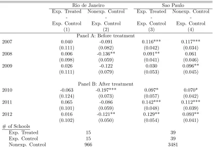
Column 1 of Table 1presents the difference in test scores for treated and control
experi-mental schools in Rio de Janeiro, and column 3 shows the same difference for schools in Sao
Paulo. Panel A presents this information for 2007 to 2009, which was before the intervention.
For Rio de Janeiro, all differences are small and not statistically different from zero, as one
would expect given random assignment. For Sao Paulo, however, there are significant
differ-ences in test scores in 2007 and 2008, suggesting that there may have been some problems
in the assignment of treatment schools. Panel B presents the results for the three years after
the implementation of the program. The comparison between treated and control schools
suggest a null effect of the program in Rio de Janeiro, and a positive and significant effect
in Sao Paulo. We should be careful in interpreting the results for Sao Paulo, however, due
to the imbalances in pre-intervention test scores.17
14It is not possible to identify the schools that participated in the “Jovem de Futuro” experiment using the
public-access ENEM microdata before 2007. For this reason, we do not consider earlier implementations of the program in Minas Gerais and Rio Grande do Sul, because we would only have one year of pre-treatment outcome.
15
For 2007 and 2008, we focus on the score on a 63-question multiple-choice test on various subjects (Portuguese, History, Geography, Math, Physics, Chemistry and Biology). Since 2009, the exam has been composed of 180 multiple-choice questions, equally divided into four areas of knowledge: languages, codes and related technologies; human sciences and related technologies; natural sciences and related technologies; and mathematics and its technologies. In this case, we consider the average score for these four areas. For each year and for each state, we standardize the test scores based on the sample of students from the experimental control schools.
16We exclude one control and two treated schools from Sao Paulo because they lack information for at
least one of these years.
Columns 2 and 4 of Table 1 present differences in test scores for public schools that did
not participate in the experiment and schools in the experimental control group. In Rio
de Janeiro, schools that (voluntarily) decided to participate in the experiment had better
outcomes prior to the intervention, relative to other schools that did not participate in the
experiment. In Sao Paulo, schools in the experimental control group were, on average, worse
than the schools that did not participate in the experiment. Interestingly, Rio de Janeiro
has 966 and Sao Paulo has 3481 non-experimental public schools, thus providing a setting
with few treated and many (non-experimental) control schools.
5.1
Empirical Monte Carlo Study
We consider an empirical MC study based on the “Jovem de Futuro” implementation.
We first estimate a probit model using schools’ average test scores in the three years prior
to the intervention as covariates. We estimate the probit model using the implementation
of the program in Sao Paulo, which was a place where the program focused on attending
schools with lower test scores, so treatment selection is a more severe problem in this case.
We also include private schools to have a larger population for the simulation study.18 Then
we exclude the treated schools and draw placebo treatments for all schools in Brazil with a
treatment selection process based on the estimated probit model. We have a population of
20,363 schools for this simulation study. Based on these simulations, we find, on average, a
difference of −0.32 points in a standardized test score when we simply compare treated and control schools under this selection process, revealing that schools that participated in this
program had, on average, worse test scores relative to other schools.
For each realization of the placebo treatment, we control the number of treated and
control observations by selecting a random sample of N1 ∈ {5,10,25,50} treated and N0 ∈
{50,500} control schools. We then estimate the nearest neighbor matching estimator with
M ∈ {1,4,10}, and calculate rejection rates based on the asymptotic distribution derived
byAbadie and Imbens (2006), and based on the randomization inference tests presented in
Section4. For each scenario, we draw 10,000 samples.
Bias and Mean Square Error
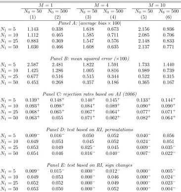
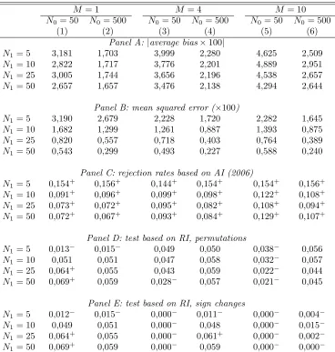
Panel A of Table 2 shows the average bias of the nearest-neighbor matching estimator.
Columns 1 and 2 has M = 1. For N0 = 50, the matching estimator for the treatment effect on the treated has a bias of around 0.01, regardless of the number of observations in the treated group, which reflects the fact that, with a finite N0, it is impossible to guarantee a perfect match in X for the treated observations and their nearest neighbors. This bias, however, equals only about 3% of the bias of a naive comparison between treated and control
observations, suggesting that, in this setting, the matching estimator is very effective in
controlling for differences in observables of treated and control schools, even when N0 is not large. Consistent with Proposition 1, the average bias shrinks to zero when we increase the
number of control observations, regardless of the number of treated observations. When the
matching estimator has more nearest neighbors, the bias increases, but it remains close to
zero when N0 = 500. This happens because, with a limited number of control observations, we end up with poorer matches when considering an estimator with more nearest neighbors.
This loss in match quality becomes less relevant when there are many control observations.
Panel B of Table 2 presents the mean square error (MSE) of the matching estimators.
While the MSE is always decreasing in N1 and N0, two competing forces come into play when M increases. On the one hand, using more nearest neighbors reduces the variance of the matching estimator. On the other hand, this increases the bias of the estimator. With
N0 = 500, since increasing M from one to ten has little impact on the bias, using more nearest neighbors — in this range — always reduces the MSE of the matching estimator.
However, with smallerN0 there are some cases in which increasingM actually increases the MSE, exposing the trade-off between bias and variance for the matching estimator.
in-creases.19 While the number of covariates does not affect our theoretical results in
Proposi-tion1, these simulations confirm the intuition that, when the dimensionality of the covariates
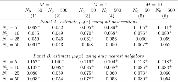
increases, a larger N0 is required to keep our approximations reliable. Finally, Appendix Ta-bleA.2presents simulations for a bias-corrected estimator, as defined in equation6.20 While
the average bias is reduced using this procedure, the effects on the MSE are ambiguous. In
particular, the bias corrected estimator may lead to higher MSE when N1 is very small and
N0 is not large. WhenN0 is large, the bias correction becomes less relevant, so the bias and MSE of the two estimators become very similar.
Inference: test size
Panels C to E of Table 2 show rejection rates for 5% tests using different inference
methods. A superscript “+” indicates a rejection rate greater than 6%, and a superscript
“−”, a rejection rate lower than 4%.21 Importantly, while the different test procedures rely
on different null hypotheses, all these null hypotheses are valid in the simulations. We discuss
in detail the implications of considering tests that rely on different null hypotheses in Section
6.
Panel C of Table 2 presents rejection rates using the test based on Abadie and Imbens
(2006).22 Rejection rates for a 5% test are higher than 13% when N
1 = 5, and around 9%
whenN1 = 10, for all values ofN0andM. This happens because the asymptotic distribution derived by Abadie and Imbens (2006) relies on N1 → ∞, even though it allows N0 to grow
19We generate three additional covariates with the same distributions of the test scores from 2007, 2008,
and 2009, but that are independent of all other random variables in the model. Then we estimate the matching estimator including these variables, in addition to the original ones, as covariates. A mismatch in these additional variables would not directly generate bias in the matching estimator. However, the addition of these variables makes it harder to find a good match in terms of relevant covariates, which might lead to higher bias.
20
We use linear least squares using only the nearest neighbors to estimate µ0(x). This is the procedure used in the teffects command in Stata.
21
While there is an asymmetry in that over-rejection is usually considered a more relevant problem relative to under-rejection, it is also important to highlight cases in which a test under-rejects, as this might imply that the test is under-powered.
22We consider in our simulations the default options of the teffect program in Stata, which uses the robust
at a faster rate than N1. When N1 increases, rejection rates go down, although they are still marginally higher than 5% even when N1 = 50. The simulations suggest that rejection rates computed using the asymptotic variance derived byAbadie and Imbens (2006) should
be considered with caution when the number of treated observations is small.
Panel D of Table 2 shows rejection rates using randomization inference test based on
permutations. Rejection rates are close to 5% in most cases. The exceptions are the scenarios
with M = 1/N1 = 5, and with M = 10/N1 ∈ {25,50}, in which the test is conservative. In both cases, the test is conservative because there are relatively few possible permutations.23
In the first case, there are few possible permutations because the dimension of ˜SN0 is small. Therefore, the test should remain conservative even when we increaseN0 even further. In the second case, the test is conservative because we end up with many shared nearest neighbors
(see Remark13). Therefore, the test would lead to rejection rates closer to 5% if we increase
N0.
Panel E of Table 2 shows rejection rates using the randomization inference test based
on sign changes, presented in Section 4.2. When the nearest-neighbor matching estimator
with M = 1 is considered, rejection rates using this test are close to 5%, except when
N1 = 5. In this case, few different group transformations exist, which explains why the test is conservative.24 When we consider matching estimators with M >1 and N
0 = 50, the test
under-rejects the null hypothesis, even for larger N1. This happens because increasing M
increases the probability that different treated observations share the same nearest neighbors,
which in turn reduces the number of group transformations. When N0 = 500, this problem becomes less relevant, and rejection rates approach 5%, when M = 4. However, the test is still conservative when M = 10. Since this comes from a higher proportion of shared neighbors when M = 10, the test would lead to rejection rates closer to 5% if we increase
23
We use the non-randomized version of the test in which we do not reject the null hypothesis in case of equality. We could guarantee the correct size if we used a randomized version of the test, as explained in Remark11.
24
N0 (except for the case with N1 = 5).
Appendix TableA.1show some over-rejection for the randomization inference tests when
we increase the dimensionality of the covariates, which is explained by the fact that the
bias is more relevant in this scenario. Again, such over-rejection does not arise if N0 is large enough. When a bias-corrected estimator is used, Appendix Table A.2also show some
over-rejection in the permutation test when N1 and N0 are small, despite the fact that the bias is smaller. When N0 is large, there is not much difference in rejection rates between the standard and the bias-corrected matching estimator. Finally, Appendix TableA.3shows
that the bootstrap test proposed byOtsu and Rai(2017) can also lead to over-rejection when
N1 is small. WhenN1 andN0 increases, rejection rates converge to 5%, which was expected given the theoretical results derived by Otsu and Rai(2017).25
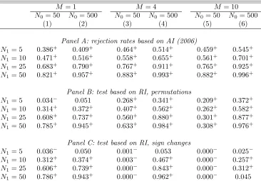
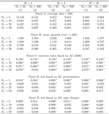
Inference: test power
Table 3present rejection rates when we assume a homogeneous treatment of 0.2 standard deviations in the students’ outcomes (that is, Yi(1) = Yi(0) + 0.2 for all i). An important caveat when comparing these different inference procedures is that inference based on the
asymptotic distribution derived by Abadie and Imbens (2006) leads to over-rejection under
the null, particularly when N1 is small. Therefore, these results should be considered with caution. As expected the power of these tests are increasing with N1. The power is also increasing with M, but at decreasing rates, which is expected given the discussion presented by Imbens and Rubin (2015) that M should not be large. Most importantly, the two ran-domization inference tests present non-trivial power in many settings in which tests that
rely on N1 → ∞ would lead to over-rejection. The only exceptions are the cases in which
25
We focus on the wild bootstrap implementation of test using the two point distribution suggested by
Mammen(1993). Another alternative proposed byOtsu and Rai(2017) would be a nonparametric bootstrap. However, with few treated and many control observations, we would likely generate bootstrap samples with no treated observations. Differently from the other tests we considered, this test must be based on a bias-corrected estimator, and it requires some properties on the estimator forµ0(x) (seeOtsu and Rai(2017) for details). FollowingOtsu and Rai(2017), we estimateµ0(x) using a linear OLS with all control observations. We also present results using the estimator forµo(x) used by default in the teffects command in Stata, which
there are few possible group changes, so that the test is conservative. Therefore, there are
settings in which the randomization inference tests may provide an important alternative to
inference methods that rely on N1 → ∞. In Section 6, we contrast these different inference procedures in more detail, providing guidance on how to evaluate the trade-offs of these
methods in different settings.
5.2
Empirical Application
Our idea is to estimate the effects of the program using a matching estimator with the
experimental treated schools as treated observations and schools that did not participate in
the experiment as control observations, therefore providing a setting with few treated and
many control observations. Moreover, we take advantage of the randomized control trial
to analyze the validity of the matching estimator and of different inference methods in this
setting. More specifically, we consider a matching estimator using the experimental control
schools as treated observations, and schools that did not participate in the experiment as
control observations. Since the experimental control schools did not actually receive the
treatment in the analyzed period, we should not expect to find significant effects in this
case.
One important caveat in using ENEM test scores is that the treatment may have affected
the probability that a student would take the exam. We do not find, however, significant
differences in the number of students who took the exam between treated and control schools
(see Appendix Table A.4). Moreover, one of our main exercises in this empirical application
is to analyze the performance of matching estimators using the experimentalcontrol schools
as the treated observations. Since the experimental control schools were not affected by the
treatment, we do not have any reason to believe sample selection should be a problem in
this case.
Table 4shows estimated effects from 2010 to 2012 using the experimentalcontrol schools
par-ticipate in the program, but were not actually treated during this period. Therefore, if the
matching estimators are valid, then we should not expect to find significant effects. In
addi-tion to the point estimates, p-values are calculated using the asymptotic distribuaddi-tion derived
byAbadie and Imbens(2006), and from the two proposed RI tests. We use test scores from
2007 to 2009 as matching variables. Interestingly, estimates for Rio de Janeiro (columns 1 to
4) generally have lower p-values using the test based on Abadie and Imbens(2006), relative
to the alternative inference procedures. In particular, a test based on Abadie and Imbens
(2006) would reject the null at 10% in two cases, while the other tests would fail to reject
the null. This is consistent with our simulations from Section 5.1, that show the test based
on Abadie and Imbens (2006) may lead to over-rejection when N1 is small. The difference in p-values across different methods is less pronounced when we consider estimates for Sao
Paulo, which is consistent with having a larger number of “treated” schools in Sao Paulo.
Finally, Table 5 presents estimated effects using the experimental treated schools as the
treated observations in our matching estimators. The effects for Rio de Janeiro are small
and not significantly different from zero, which is consistent with the experimental results
presented in Table1. For Sao Paulo, some results for 2011 and 2012 are significant, depending
on the specification. While positive, the estimates for Sao Paulo are generally smaller than
the experimental results presented in Table 1, which is consistent with the imbalances in
pre-treatment outcomes for the experimental sample.
6
Choosing Among Alternative Inference Methods
The different test procedures we consider present important trade-offs in terms of size
distortion, power, and the underlying null hypothesis they rely on. In light of the theoretical
properties derived in Section 4, and of the empirical evidence presented in Section 5, we
provide guidance on how to evaluate these trade-offs. First, note that tests based on the
proce-dure proposed byOtsu and Rai (2017), are valid to test the null hypothesis τ({Xi}i∈I) = 0, provided both N1 and N0 are large enough so that the asymptotic approximations are reli-able. The randomization inference tests, in contrast, rely on more stringent null hypotheses.
Therefore, if we believeN1 is large enough so that this approximation is reasonable, then we should use one of these tests that rely on N1 → ∞, instead of the randomization inference ones. In our simulations, for example, there is only a slight over-rejection when N1 = 50, so the advantage of using an inference method that is valid to test a less stringent null
hypothesis should dominate.
When N1 is not that large, then the over-rejection of tests that rely onN1 → ∞becomes more relevant, so it may be reasonable to consider alternative inference procedures that
allow for N1 fixed. The randomization inference test based on sign changes relies on a slightly more stringent null hypothesis, that the average treatment effect for each value of
Xi is equal to zero. However, in light of Remark 15, if τ({Xi}i∈I) = 0, but the null is false because treatment effects are heterogeneous across Xi, then the test would under-reject. This means that such test would only reject at a rate greater than α when it is actually the case that τ({Xi}i∈I) 6= 0 (asymptotically, with N1 fixed and N0 → ∞). Therefore, if the goal is to test the null τ({Xi}i∈I) = 0, then we should not expect over-rejection for any value ofN1. This test would have low power if N1 is very small, or if N0 is not very large, so that many treated observations share the same nearest neighbors. Since the proportion of
shared nearest neighbors is increasing with M, this provides another reason to avoid using matching estimators with large M (see Imbens and Rubin (2015) for other reasons to avoid using large M). In our simulations, the test based on sign changes becomes an attractive alternative when N1 ∈ {10,25}. In these cases, it has the correct size and non-trivial power, while tests that rely onN1 → ∞presented relevant size distortions. WhenN1 = 5, however, this test is underpowered, so it should not be used.
Finally, the randomization inference test based on permutations is the only one that
very stringent null hypothesis, which implies that we may reject at a rate greater than α
even when τ({Xi}i∈I) 6= 0 (see Remark 7). Therefore, this test should only be used when alternative methods either lead to significant over-rejection or provide trivial power.
7
Conclusion
We consider the asymptotic properties of matching estimators when the number of
con-trol observations is large, but the number of treated observations is fixed. In this setting,
the nearest neighbor matching estimator is asymptotically unbiased for the ATT under
stan-dard assumptions used in the literature on estimation of treatment effects under selection
on unobservables. Moreover, we provide tests, based on the theory of randomization under
approximate symmetry, that are asymptotically valid when the number of treated
obser-vations is fixed and the number of control obserobser-vations goes to infinity. The different test
procedures we consider present important trade-offs in terms of size distortion, power, and
the underlying null hypothesis they rely on. We, therefore, provide guidance on on how to
evaluate the trade-offs among these different test procedures in specific settings.
Our results are also relevant for Synthetic Control (SC) applications. Following
Doud-chenko and Imbens(2016), the SC and the matching estimators are nested in a framework in
which the estimated counterfactual outcome for the treated observation is a linear
combina-tion of the outcomes for the controls. In the framework of Doudchenko and Imbens (2016),
if we consider linear combinations of the controls such that the weights given to observations
with large discrepancies in pre-treatment outcomes relative to the treated units go to zero,
then, following the same arguments as we do for the matching estimator, the estimator is
asymptotically unbiased if treatment assignment is “as good as random,” conditional on
this set of pre-treatment outcomes.26 Moreover, under these conditions, the randomization
26If however, treatment assignment is only “as good as random” conditional on a set of common factors
pre-inference test based on sign changes remains asymptotically valid when the number of
con-trol units goes to infinity. Given recent concerns regarding the validity of the placebo test
proposed byAbadie et al. (2010) (see, for example,Ferman and Pinto(2017) and Hahn and
Shi (2017)), the randomization inference test based on sign changes may provide a feasible
alternative when there are multiple treated units and a large number of control units.27 The
only caveat is that a very large number of control observations are needed when the number
of pre-treatment periods is large, so that approximations remain reliable.
References
Abadie, A., Diamond, A., and Hainmueller, J. (2010). Synthetic Control Methods for Com-parative Case Studies: Estimating the Effect of California’s Tobacco Control Program.
Journal of the American Statiscal Association, 105(490):493–505.
Abadie, A. and Imbens, G. W. (2006). Large sample properties of matching estimators for average treatment effects. Econometrica, 74(1):235–267.
Abadie, A. and Imbens, G. W. (2011). Bias-corrected matching estimators for average treatment effects. Journal of Business & Economic Statistics, 29(1):1–11.
Barros, R., de Carvalho, M., Franco, S., and Rosal´em, A. (2012). Impacto do projeto jovem de futuro. Estudos em Avalia¸c˜ao Educacional, 23(51):214–226.
Bodory, H., Camponovo, L., Huber, M., and Lechner, M. (2018). The finite sample per-formance of inference methods for propensity score matching and weighting estimators.
Journal of Business & Economic Statistics, 0(ja):1–43.
Bugni, F. A., Canay, I. A., and Shaikh, A. M. (2018). Inference under covariate-adaptive randomization. Journal of the American Statistical Association.
treatment periods increases, even if the number of control units is fixed, whileGobillon and Magnac(2016) show provide conditions such that this perfect pre-treatment match is achieved when number of control units and the number of pre-treatment periods go to infinity. See alsoFerman and Pinto(2016) for a discussion of the conditions for asymptotic unbiasedness for the SC estimator when the number of control units is fixed, and a perfect pre-treatment match is not assumed.
Busso, M., DiNardo, J., and McCrary, J. (2014). New Evidence on the Finite Sample Properties of Propensity Score Reweighting and Matching Estimators. The Review of Economics and Statistics, 96(5):885–897.
Canay, I. A. and Kamat, V. (2018). The Review of Economic Studies. Forthcoming.
Canay, I. A., Romano, J. P., and Shaikh, A. M. (2017). Randomization tests under an approximate symmetry assumption. Econometrica, 85(3):1013–1030.
Chernozhukov, V., Wuthrich, K., and Zhu, Y. (2017). An exact and robust conformal inference method for counterfactual and synthetic controls.
Conley, T. G. and Taber, C. R. (2011). Inference with Difference in Differences with a Small Number of Policy Changes. The Review of Economics and Statistics, 93(1):113–125.
Dehejia, R. H. and Wahba, S. (1999). Causal effects in nonexperimental studies: Reevaluat-ing the evaluation of trainReevaluat-ing programs. Journal of the American Statistical Association, 94(448):1053–1062.
Dehejia, R. H. and Wahba, S. (2002). Propensity Score-Matching Methods For Nonexperi-mental Causal Studies. The Review of Economics and Statistics, 84(1):151–161.
Doudchenko, N. and Imbens, G. (2016). Balancing, regression, difference-in-differences and synthetic control methods: A synthesis.
Ferman, B. and Pinto, C. (2016). Revisiting the Synthetic Control Estimator. MPRA Paper 73982, University Library of Munich, Germany.
Ferman, B. and Pinto, C. (2017). Placebo Tests for Synthetic Controls. MPRA Paper 78079, University Library of Munich, Germany.
Ferman, B. and Pinto, C. (2018). Inference in differences-in-differences with few treated groups and heteroskedasticity. The Review of Economics and Statistics, forthcoming.
Ferman, B. and Ponczek, V. (2017). Should we drop covariate cells with attrition problems? Mpra paper, University Library of Munich, Germany.
Frolich, M. (2004). Finite-sample properties of propensity-score matching and weighting estimators. The Review of Economics and Statistics, 86(1):77–90.
Gobillon, L. and Magnac, T. (2016). Regional Policy Evaluation: Interative Fixed Effects and Synthetic Controls. Review of Economics and Statistics. Forthcoming.
Hahn, J. and Shi, R. (2017). Synthetic control and inference. Econometrics, 5(4).
Huber, M., Lechner, M., and Wunsch, C. (2013). The performance of estimators based on the propensity score. Journal of Econometrics, 175(1):1 – 21.