Issues in the Bayesian forecasting of dispersal after a nuclear accident

(1)

University of Warwick institutional repository:

http://go.warwick.ac.uk/wrap

A Thesis Submitted for the Degree of PhD at the University of Warwick

http://go.warwick.ac.uk/wrap/73485

This thesis is made available online and is protected by original copyright.

Please scroll down to view the document itself.

(2)

ISSUES

m

THE BAYESIAN FORECASTING

of

DISPERSAL AFTER A NUCLEAR ACCIDENT

Thesis submitted in fulfilment of requirements for the degree of

Doctor of Philosophy

Ali S. Gargoum

Department of Statistics

University of Warwick

(3)

List of Figures

1.1 Model Structure of RODOS . . . . . 3

3.1 The plume as represented by puffs 34

3.2 Puff pentification . . . 41

3.3 Plume trajectory and pentification 43

4.1 An illustration of some graph-theoretical terms 52 4.2 An ID I . . . . 55 4.3 Graphs of decomposable and non-decomposable IDs 57 4.4 An undirected graph with diques satisfying the RIP 59 4.5 An ID J and its junction graph . . . 60 4.6 An ID of early emissions and its junction tree . . 66

5.1 A plot of distances between N[O, 1] and N[O,

0'2] .

77

6.1 Forecast function ft{k) = 1 - (O.5)k . . . . 85

6.2 Forecast function ft{k) = (kjO.90)(O.90)k 86

(8)

6.5 Forecast emission from simulated noisy stack readings using example (1) 99 6.6 Retrospective fitted concentration . . . .

6.7 Mangement of uncertainty of release height

7.1 Tip of a. decomposable graph 7.2 Tip of a clique tree . . . .

7.3 An illustration of the OBLINK opera.tor

100 101

(9)

List of Tables

7.1 Positions of detector points on a grid . . . 138 7.2 Comparisons of concentration forecasts using two models. 139

(10)

Acknowledgements

I am deeply indebted to my supervisor, Professor Jim Smith. His excellent guidance, sustained encouragement and friendship made this thesis possible and these years of research a very pleasant experience.

I thank Professor P. J. Harrison for many discussions, lessons and for his help in using the two software packages, PROF and BATS.

I acknowledge the help of D. Ranyard from Leeds University in coding some of the new operators and algorithms proposed in this thesis.

I must also thank the staff of the Statistics Department at the University of Warwick and my fellow research students.

I would like to express my gratitude to the University of Garyounis (Benghazi) for giving me the opportunity to carry out this research and for their financial support.

Finally, I would like to thank my family for always supporting and encouraging me.

Declaration

(11)

(12)

Summary

This thesis addresses three main topics related to the practical problems of modelling the spread of nuclear material after an accidental release.

The first topic deals with the issue of how qualitative information (expert jUdgement) about the development of the emission of contamination after an accident can be coded as a Dynamic Linear Model (DLM). An illustration is given of the subsequent adaptation of the expert judgement in response to the incoming data. Moreover, the height of the release at the source can be a key parameter in the subsequent dispersal. We addressed uncertainty on the release height using the Multi-Process Models framework. That is we included several models in our analysis, each with a different release height. The Bayesian methodology uses probabilities representing their relative likelihood to weight these and updates the probabilities in the light of monitoring data. A brief illustration of testing the updating algorithm on simulated contamination readings is provided.

The second topic concerns the demands of computational efficiency. We show how the Bayesian propagation algorithms on a dynamic junction tree of cliques of variables (representing a high dimensional Gaussian process), as provided by Smith et al. (1995), can be generalised to incorporate the case when data may destroy neat dependencies (i.e. when observations are taken under more than one clique). Here we introduce two classes of new operators: exact and non-exact (approximations) which act on this high dimensional Gaussian process, modifying its junction tree by another tree which allows quicker probability propagation. We also develop fast algorithms which can be defined by approximating Gaussian systems by cutting edges on junctions. The appropriateness ofthe approximations is based on the Kulback-Leibler/Hellinger distances.

Some of these new operators and algorithms have been implemented and coded. Preliminary tests on these algorithms were carried out using arbitrary data, and the system proved to be highly efficient in terms of P.C. user time.

The third topic concentrates on generalisations from a Gaussian process. It proposes, as a good approximation, an adaptation of the Dynamic Generalised Linear Models (DGLMs) of West, Harrison, and Migon (1985) for updating algorithms on a dynamic junction tree. The Hellinger distance is used to check the accuracy of the dynamic approximation.

(13)

Chapter

1 Introd uction

This introduction gives a brief background to the original application which has moti-vated the research, presents the aims of the thesis, and then provides an outline of the whole work.

1.1 Background

In the event of an accidental release of radioactive pollutants or chemical gases, coun-tries will be concerned about the danger of environmental contamination, and in this respect interest centres on the prediction of the distribution of the radioactive emissions reaching these countries and the identification of regions where contamination is most likely to exceed certain prescribed levels.

(14)

Com-mission of the European Communities (CEC) to establish a number of projects to build Decision Support Systems (DSSs) and methodologies for use in the event of a future accident. One of these is the RODOS project.

RODOS is a Real-time On-line DecisiOn Support system for nuclear emergencies in Eu-rope, being jointly developed by some European institutions with support of the CEC. It is designed as an integrated software environment, which allows the implementation of software (external programs) developed by the contractors.

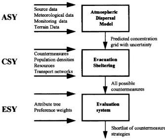
RODOS comprises three subsystems (see Ehrhardt et al., 1993).

(i) The analysis subsystem (ASY). The main task of this component is to provide continually updated forecasts of the spread of any contamination. The ASY con-sists of an atmospheric dispersion model such as Rimpuff model-will be discussed later- which is the prediction model; it predicts concentration of contamination both at present and in the future. The predictions are based on different sources of information:

• An estimate of the source term. This comprises the mass, and the height of the release, and is most likely to be expert judgement.

• Meteorological data.

• Geographical data from a Geographical Information System (GIS).

The output of the ASY is in a form of a grid of concentrations with an associ-ated uncertainty distribution. The grid becomes one of the inputs to the next subsystem, the CSY.

(15)

pos-sible countermeasures (sheltering and evacuation for the local population; food bans; etc.) and to quantify the benefits and drawbacks of various countermeasure combinations. The CSY then outputs a list of all possible countermeasures for input to the next subsystem, the ESY.

(iii) The evaluation subsystem (ESY). The main task ofESY is to evaluate the different countermeasures strategies. Figure 1.1 below shows the structure of RODOS.

Source data ~

ASY

Meteorological data

Monitoring data Terrain Data

~

Countermeasl.U'es

CSY

Population densities

Resources

Transport networks

~ ~

Attribute tree

ESY

Preference weights

~

Atmospheric Dupe"aI

Model

Predicted

,r

grid with

Evacuation Sheltering

concentration uncertainty

All possib

,r

counterm Ie easures

Evaluation

.ystem

Shortlist of countermeasure

"

strategies

Figure 1.1: Model Structure of RODOS

[image:15.519.102.437.251.535.2]

(16)

All the sources of information mentioned in ASY above are not considered to be one hundred per cent accurate. There are several uncertainties associated with them. For instance, RODOS contains an algorithm which describes the dispersal of radia-tion in the atmosphere. Such algorithms can only ever be approximaradia-tions of what is happening, and other methods must be incorporated to control them effectively. Also, uncertainty may arise from the lack of knowledge of source term characteristics (the re-lease characteristics) and the surface characteristics that affect the pollutant behaviour; etc.

Within the framework of RODOS, Smith & French (1993) investigated the feasibil-ity of managing the uncertainties relating to the key variables which are important for decision making in the short term, and of assimilating data as they became available using Bayesian methodology. The Bayesian methodology can tackle a number of issues of interest, for example: data assimilation, expert judgement, model uncertainty, etc. The authors designed the ASY module based upon the RIMPUFF model with Bayesian updating in the light of monitoring data in order to address the following questions:

• What is the likely spread of contamination ?

• How can the prediction be updated in the light of monitoring data?

• What are the uncertainties in the prediction ?

The authors have been able to combine the Dynamic Linear Model (DLM) methodology with the RIMPUFF model to address all three questions.

(17)

model used within RODOS. RIMPUFF approximates the continuous release of air-borne substances (such as radiation) by a discrete series of puffs. Puffs may contain different masses reflecting the uneven pattern release from the source. Different

pa-rameters can be associated with each puff, enabling characteristics of the windfield or local information gathered for monitoring data to be incorporated. The concentration distribution in each individual puff is assumed to be Gaussian, and puffs grow in size over time.

A further feature of the RIMPUFF model is pentification. When a puff reaches a cer-tain diameter, it is approximated by five smaller child puffs. Cercer-tain percentages of the mass of the parent are distributed amongst its children. These percentages can be adjusted in the light of observational data. The adjustment is controlled by incorpo-rating a Bayesian probability distribution over the model. As new data arrive (ground and air contamination readings), the puff mass estimates will be revised.

(18)

sets arrive on one clique at a time.

1.2 Aims

The basic issues of this research are as follows:

Firstly, to model the qualitative information of the experts of how they believe the emission of contamination will develop over time.

Secondly, to build a probabilistic expert system which is able to:

• generalise current exact Bayesian propagation algorithms on dynamic junction trees of cliques as described in Smith et al. (1995) to even faster algorithms (computational efficiency) .

• modify these exact algorithms (to approximation algorithms) when the condi-tional independence structures of the junction trees may be destroyed.

Thirdly, to generalise these linear updating algorithms to allow dispersal concentra-tion readings to be a non-Gaussian process. The Dynamic Generalised Linear Model (DGLM) of West, Harrison and Migon (1985) will be modified to give closed form updating solutions which can be used on dynamic junction trees for a variety of non-Gaussian processes.

1.3 Outline of the Thesis

(19)

In Chapter (3) we introduce the traditional dispersal models in general, with par-ticular emphasis on puff models. A statistical model which embeds physical models to handle uncertainties from different sources is defined and described.

Chapters (4) and (5) provide a necessary background for the development of the new material presented in Chapters (7) and (8). Chapter (4) looks at some graph-theoretical results on graphical modelling; Chapter (5) is devoted to information divergence, where definitions and properties of some separation measures are given.

Chapter (6) deals with describing the source emission process by considering several scenarios of expert judgement about the development of the release. An illustration of adaptation with simulated data is given for different emission profile shapes. Also in this chapter we discussed uncertainty management of key parameters of the emission process namely the release height.

Chapter (7) introduces two classes of new operators (exact and non- exact) which act on a high dimensional Gaussian process transforming its junction tree to another tree which accommodates data induced dependences (conditional independences im-plicit in the clique structure before the data arrived are no longer necessarily valid af-ter the data are observed). Also we proposed a new approximation scheme using edge deletion (neglecting weak dependences) in order to achieve computational efficiency.

In Chapter (8) we adapt the updating algorithms of Dynamic Generalised Linear Models (DGLMs) to updating algorithms on dynamic junction trees. The appropriate-ness of the dynamic approximation is based on the Hellinger metric.

(20)

Chapter

2 Dynamic Linear Models: A Brief

Review

2.1 Introduction

The Dynamic Linear Model (DLM) offers many facilities which will be used through-out this thesis. These include the use of expert judgement to start up the system; the construction of complex models from simple components using the superposition prin-ciple; the intervention analysis; simple sequential updating recursions; and Dynamic Generalised Linear Models (DGLM).

(21)

2.2 Bayesian Forecasting and Dynamic Models

In the control literature, linear dynamic systems are used by control engineers to moni-tor and control the state of a system or a process as it changes over time. To determine whether a system is operating satisfactorily, it is necessary to know the behaviour of the system at any time. For example, in the case of a nuclear accident, the state of the system may be the position of the plume of the contaminated material. The state of the system is random because physical systems are usually subject to random disturbances and the observations taken on the system are often noisy observations.

Making inference about the state of the system from noisy measurements and con-sequently deriving the predictive distributions of future observations is an important problem. Explicitly, the problem can be expressed in a general dynamic form as

(2.1)

(2.2) where the first equation relates the observations

lit

with the state 8t of the system, and the second relates the state variables at time t and those at time t - 1. In the first equation, called the observational equation, the quantity lit reflects observational error.

The second equation, called the state equation, assumes that the state at time t cannot be determined exactly by the state at time

t -

1 because of the effect of many unknown factors summarised in the random error

"'t.

(22)

from the past that is needed in order to predict the future.

The objective of the analysis is to make inference about 8_tH, k ~ 0 given the set of observations Yl,' .. , Yt-l. Originally Kalman (1960) derived a recursive algorithm to estimate the state of the system using the properties of orthogonal projection on linear spaces. Mehra (1979) summarised the key aspects of this approach to forecast-ing (known as the filterforecast-ing approach) with particular emphasis on the original work done by Kalman. The idea of using the state-space engineering representation and the principle of recursive updating of information in statistics did not appear until the early to mid 1970's. Harrison & Stevens (1976) adopted a stat~space representation in the context of Bayesian inference to describe the Dynamic Linear Model (DLM). An intrinsic difference between Harrison & Stevens's approach and that of Kalman was that Kalman expressed his recurrence relationships in terms of moments, whereas Harrison & Stevens used the same updating equations to describe the evolution of a fully probabilistic Gaussian process.

Bayesian methods are often useful in forecasting problems where there is little or no useful historical information available at the time the initial forecast is required. In this situation the early forecasts must be based on subjective assessment and experienced judgement. As the time series information becomes available, we then use Bayes the-orem to combine our prior information with the observed data through the likelihood function - the joint probability of the data under the stated model assumptions- to give the posterior distribution or information. This prior to posterior process can be expressed as

(23)

An example of this process is the forecasting of contaminated material which has a short life after a nuclear accident. An experienced judgement is needed at the beginning of the emission process. This is a process based on using Bayes theorem for updating a degree of belief expressed by a probability distribution in the light of new information. Bayesian forecasting uses Bayesian inference to study systems through dynamic models.

2.3 The Univariate DLM

2.3.1 Definition

Following the notation and terminology of West & Harrison (1989), the standard normal DLM is described as follows.

Let yt,

t

= 1,2, ... represent a time series of scalar observations. At time

t

we have the following defining equations

(2.3)

(2.4)

where the quantity 8t is an nrdimensional state parameter vector evolving through time according to the evolution or system equation (2.4). In the application we have in mind, the dimension of 8t will have the novel feature that it will depend on t as a function of the parameter of the model. Gt is the known nt x nt system matrix of the model defining the systematic component of the evolution and Wt is a stochastic term which describes random changes in the state vector, and which provides an increase in uncertainty over the time interval as 8_{t -}₁changes to 8t • Conditional on the past information Dt -1

(24)

is a known covariance matrix which provides the measure of increased uncertainty or loss of information. The structure of this matrix is defined using discount factors as discussed in Section (2.4). The state vector relates to the observation at time t via equation (2.3), systematically through the known, nt-dimensional regression vector F_t and stochastically via the observational noise term Vt. Typically (VtIDt-d '" N[O,

Yt]

with

Yt

known apart from a constant or a scalar precision parameter which may be estimated (Harrison & West 1986, 1987). The mean response at t is Itt = F;8t , which is simply the expected value of yt in equation (2.3) and defines the level of the series at time t. Finally, the sequences {vt} and {wt} are usually assumed uncorrelated and mutually uncorrelated. The univariate DLM can then be characterised by a quadruple

which is known at time

t.

This quadruple, together with the initial information (80IDo) '"

N[mo, Co], where mo is the prior expectation for

8₀and Co is its covariance matrix, define the DLM, assuming the initial distributions for the state to be independent of Vt and Wt.

2.3.2 Model Updating

Suppose that at each time t an observation yt = _{Yt is made such that Dt}= {Yt, Dt-t}. Then, with {F,G, V,

Wh

known for all t the, DLM can be updated as follows.

1. At time t - 1 we have a posterior distribution for the state vector given as

(25)

2. Using equation (2.4), prior distribution on the state vector for time

t,

(8

t

ID

t

-d

will be normally distributed with defining moments

Gtmt-t

GtGt-tGT

+

Wt

3. At this stage we forecast the expected new observation according to equation (2.4). The one-step ahead forecast distribution for

(YtID

t -.) will be normally distributed with defining moments

E[YtIDt-tl

-

it

Var[YtID

t -1] Qt

Frat

FrRtFt

+

\.'t.

4. When the new observation Yt

=

Yt is taken, the state vector is updated according to Bayes' rule, and from the joint normal distribution of Yt, 8t we obtain the posterior distribution at time

t

for 8t

where

mt = at

+

At(Yt - It)

Gt = Rt - AtQtAr·

with At = RtFtQt1 known as the Kalman filter or adaptive coefficient.

(26)

2.3.3 Forecast Distributions

Definition

The forecast function ft (k) is defined for all integers k ~ 0 and for any current time t as

where

is the mean response function at time t

+

k.

For k strictly greater than 0, the forecast function is defined as

The form of the forecast function in k plays a major role in defining DLMs. It is considered as a guide to the appropriateness of a particular model in any application. The following theorem provides the full forecast distributions for the series Yt and the state vector 8t . Examples of this will be given in Chapter (6).

Theorem 2.1. For each time

t

and k ~ 1, the k-step ahead distributions for 8t+k and Yt+k, given Dt are given by

(a)

State distribution: (8t+kIDt) fV N[at(k), Rt(k)],

(b) Forecast distribution: (Yt+kIDt) fV N[Jt(k), Qt(k)],

(27)

and

where

Ot(k) Gt+kOt(k - 1),

Rt(k) Gt+kRt(k - I)G;+k

+

Wt+k,

with starting values Ot(O)

=

mt and Rt(O)

=

Ct. In the special case that the system matrix Gt is constant Gt = G for all

t,

then for k ~ 0,

so that

ft(k) = F;+kGkmt.

Proof. See West & Harrsion (1989), p.ll5.

If both Ft and Gt are constants, then the DLM is known as time series DLM or TSDLM. The forecast function of the TSDLM has the form

2.4 The Discounting Concept

(28)

models a decay of information between observations. Recalling that

when there is no system error, then _Rt

=

GtCt-1G;' This means that _Wtintroduces uncertainty so that the quantity GtCt-1Gr can be considered as a discounted Rt with a discount factor 8,0

<

8

<

1. Thus _Rt= GtCttGT so that Wt = GtCt_1Gr(1s6).

In particular, in the case of a steady model with Ft

=

Gt

=

1, we have

Rt

=

¥

so that Wt

=

Ct_t{8-1 - 1).

2.5 Dynamic Estimation of Variance

So far we have assumed that the observation variance

lit

is known. But in most ap-plications this is not the case. Several approaches to learning on line about

lit

have been suggested (see, for example, Ameen & Harrison, 1985). A tractable fully Bayesian learning mechanism when the variance is constant is available.

In the context of our application, a conjugate prior to posterior analysis with an unknown variance is possible in a limited sense if we use the following parametrisation of the distribution of a noisy observation

Yi

and a vector

qt

of masses of contamination. This is an obvious modification of the algorithms of De Groot (1971) and West & Harrison (1989).

Observation

(29)

Vt an unknown parameter whilst, lit and the constant regression vector F are assumed

to be known. It is obvious that the larger the value of Vt, the larger the conditional

variance of yt. In more complex models, lit will be a function of various characteristics of the distribution of

qt"

State Information

Assume that

(2.6)

(2.7)

Updating Equations

where

(2.8)

(2.9)

with

Rt,

lit,

F, at

defined as before and

The parameters of Vt are updated using the equations

1

(2.10)

at

-

at-l

+

2

(30)

h Yt-FTmt

were ft = F1' F l ·

(Vt+ Rt)l 2

Note that this distribution is modified in the light of the normalised residual associated with Yt. The expectation E[VtIDt]' in particular, is given by (Qf~1) which, by repeated substitution in (2.10) and (2.11) gives

Setting Qo = 1 and letting

f30

---+

0 (a vague prior distribution on Vt initially) we obtain

which is the naive estimate of (VtIDt) based on normalised residuals.

2.6 Model Specification and Design

(31)

Theorem 2.2. If a TSDLM has a 2-dimensional state space, the state space can be linearly transformed so that its forecast function can be written as

where TnT = (mtl' mt2), and F and G having one of the following forms

i) F = ( : ). G = ( : ' : , )

il) F

= ( : ) .

G = ( : : )

iii)

F

= (

1 ), G

= ). (

cosw sin w )

o

-sinw cosw

where AI, ).2, ). and ware real. The forecast functions associated with these are respec-tively

iii)

ft(k) = [mtl cos(kw)

+

mt2sin(kw)]).k

An alternative expression for the forecast function (iii) above is

(32)

Example 1. This is an example of a damped growth model where the forecast func-tion rises from zero to a maximum height at time k* and then goes down exponentially. Here the forecast function has the form

with FT = (1, O),fflt = (mtl' mt2) and G as in (ii) above (a 2 x 2 Jordan block matrix with A diagonals) where 0

<

A

<

1.

Notice that the prior values of the initial state vector 8₀can be chosen so as to put mt2 = O.

Example 2. In this case the forecast function rises to an asymptotic value. It has the

form

/t(k) = Atmn

+

mt2

with FT

=

(1,1) and G as in (i) above where 0

<

Al

<

1, A2

=

1.

Usually we set mOl

=

-m02 so that this gives a (non-negative) expected exponential rise from an initial value of zero to an asymptote mt2.

2.7 The Superposition Principle

(33)

Consider the h time series

Yit

for integer h

>

1 generated by the DLM {Fi,Gi,

Vi,

Wilt with state vectors Bit of dimensions ni for i = 1, ... , h. Assume that for all distinct i

and j (1 ::; i,j ::; h) the series Vit and Wit are mutually independent of the series Vit and Wjt. Then the series

h

Yt

=

EYit

i=1

follows a DLM {F,G, V,

Wh

with a state vector given by

of dimension n = n1

+ ...

+

nh such that

Gt blockdiag{Glt, ... ,Ght},

Wt - block diag{Wlt , ... , Wht}

Proof. See West & Harrison (1989), p.184.

This principle is very useful since it provides a way of building up complex models for simple components. For instance a superposition of the models in examples (1) and (2) above has a regression vector

FT = (1,1,1,0)

and a system matrix

o

1 0 0

G=

o

0 A 1

(34)

In Chapter (6) we will discuss a range of these models to use in different cases.

2.8 Dynamic Generalised Linear Models (DGLM)

To generalise the concept of the DLM to non-normal distribution on the observed series and the state vector, West, Harrison & Migon (1985) proposed the Dynamic Generalised Linear Models (DGLM) which are essentially a dynamic and Bayesian version of the Generalised Linear Models (GLM) in Neider & Wedderburn (1972). In their generalisation, West, Harrison and Migon made no distributional assumptions about the n- dimensional state vector 8t apart from the first two moments, whilst the observables {Yi} were assumed to have a full distribution specification. Explicitly, the authors assumed that observations come from exponential family distribution -although their algorithm holds in general - with a density

(2.12) where "It and

Vt

>

0 are respectively the natural parameter and the scale parameter of the distribution, b(Yt!

Vt),

and

a(.,,)

are known functions. Here we assume that

Vt

or equivalently

l't-

1 = <Pt is a known precision parameter for all

t.

The system equation is as

(35)

Define At

= FT8

t as the linear score where Ft is a known n x 1 regression vector as defined in the standard DLM, and the link function g(.) as

(2.14)

where g(.) is a known, continuous and monotonic function mapping 17t to the real line. Then the observation model is defined by (2.12) and (2.14) while the system equation is defined by (2.13). Here we note that the standard DLM defined by (2.3) and (2.4) is a special case for which the distribution in (2.12) is N[At,

Vt],

the distributions of 8t and Wt are normal, and g(.) is the identity mapping.

West, Harrison and Migon (1985) reformulates the standard sequential procedure for the DLM and extended it to the non-normal case. In their analysis, the authors drop the normality assumption of the state vector. Similarly, the distribution of the error in the system equation is now only partially specified in terms of its first two moments. An alternative interpretation of their approach assumes that the random quantities {8t } defined in the system equation (2.13) are Gaussian and treats the whole process as approximate (see Smith, 1992 and Chapter 8). Under either interpretation the model updating is the same.

2.8.1 The DGLM updating

Suppose that

and the evolution of the model is defined by assuming that

(36)

where at

=

Gtmt-l and R t

=

GtGt_1GT

+

Wt. A full system of recursions is summarised in the following steps:

i) Under (2.14), At and 6 have a joint prior distribution which is partially specified in terms of the first two moments so that

ii) In order to obtain the one-step ahead forecast distribution we need the distribution of ("7tIDt-t). But this distribution is only partially specified since the full distribu-tion form of

At

=

g("7t)

is not necessarily known. Therefore further assumptions about the prior distribution of

At

are needed. A conjugate prior for

At

is supposed to have the form

(2.15)

for some defining parameters

O:t, Pt

and a normalising constant

c(O:t, Pt).

The defining parameters are chosen such that

The one-step ahead forecast distribution can now be obtained via

(37)

iii) Observing Yt = Yt. find the posterior for

""t

in the conjugate form

Denote the posterior mean and variance for At

=

g(""t) by

Ii

E[g(77t)lDt]

q;

Var[g(llt)IDt]

iv) Using the joint posterior distribution for At and 9 we can obtain the posterior moments for (9tIDt) as

p(At, 9tlDt ) oc p(At.9tIDt-t}p(YtIAt)

oc [P(9t

I

At. Dt-1)p(At!Dt-t}]p(YtIAt) oc p(9tIAt. Dt-1)[P(AtIDt-t}p(YtIAt)] oc p(9tIAt. Dt-l}P(AtIDt}.

Here 9t is conditionally independent of Yt given At and Dt - 1 • The posterior

dis-tribution of 9t is

(2.17)

The second probability density in the integrand can be obtained from step (iii) above. The first probability density is not always fully specified. but we only need its first two moments in order to obtain the first two moments for the posterior distribution of (9t IDt). The first two moments for (9t IAt. Dt-d can be estimated from standard Bayesian techniques. A detailed discussion of the Linear Bayesian Estimation (LBE) of moments of (9t IAt. Dt -1) is given in West & Harrison (1989). p.561. The LBE of the conditional mean E[9t_{IAt. Dt- 1]}is given by

(38)

for all At. The estimate of the variance is given by

for all At. Now from (2.17) we have

E[E{8

_{tIAt, Dt-dlDtl}

Var[E{8

_{tIAt, Dt-dlDtl}

+

E[Var{8

tIAt, Dt-dlDtl

and these can be estimated by substituting the LBE estimates as follows:

mt E[E]

and

Ct - E[V]

+

Var[E]

This step completes the updating procedure.

(39)

computational efficiency. Typically these methods, though accurate, are relatively slow and so are not currently applicable to the real time problem we have in mind here.

2.9 Multi-Process Models

In many cases, the modeller has in mind not just a single model, but several models corresponding to different possible scenarios which might explain a time series, and not just a single model. Harrison & Stevens (1976) introduced the multi-process model methodology for discriminating between rival DLMs M(i)

(i

=

1,2, ... , m) and

con-sidering them for the series simultaneously. The authors distinguished two classes of multi-process models, Class I and Class II, that are different in structure. In this thesis we are only concerned with Class I, where the class of alternative models is constant in time.

A

brief discussion of this class follows (see also West & Harrison, 1989, p.439). Let the process

{¥i},

(t =

1,2, ... ) follow a DLM Mt(a), where a are uncertain defining parameters of the model (e.g. discount factors, elements of a constant system matrix G, ... etc.). The precise value 0 = 00 is uncertain. Let the finite discrete set

A=

{Ol, ...

,am} denote the parameter space. Define

i)

The probability that the process follows the model M(i) given D_{t -}₁as

(i= 1, ... ,m)

ii)

Z as a vector of quantities of interest, for example the state vector 8t , a future observation

¥i+k,

k

>

0, ... etc.

(40)

1. The posterior probability of M(i) is updated via

where p(Ytlai, Dt-t} is the predictive density for Yt assuming the model M(i).

2. The marginal posterior densities are m

p(ZIDt) = Ep(Zlai,

Dt)p~i)

i=l

which are discrete probability mixtures of the standard T or normal distributions.

For example, in our application the emission process of the contaminated material after an accident can be modelled as a DLM which will lead to estimates of source term profile and predictions of the contamination spread. However, the model does not consider the uncertainty of the release height. One solution to this problem is to run a multi-process model which lets the mixing value a be the height. Each model in this set will be given a prior probability representing expert judgement on the likely height. These probabilities will then be updated in the light of monitoring data. By this means the data will give weights to most likely models. Details are given in Chapter (6).

(41)

Chapter 3 A Bayesian Forecasting of

Atmospheric Dispersion

3.1 Introduction

In the case of environmental disasters of different types (e.g. nuclear or chemical acci-dents) appropriate countermeasures must be taken to mitigate the consequences to the population and environment. A quick and accurate prediction of the dispersion of the contaminated material is crucial

Conventional atmospheric dispersion models (physical models) are widely used for fore-casting toxic contamination and obtaining results in real-time with varying degrees of accuracy. These models are deterministic, and one of the most significant problems associated with their use in prediction is the large degree of uncertainty inherent in their predictions.

(42)

concentra-tion observed at a given time and locaconcentra-tion downwind of a source cannot be predicted with precision (Chatwin, 1982). Concentration is a random quantity which should be described statistically or in a probabilistic framework rather than deterministically. Of primary importance is the need to define and reduce the uncertainty associated with predictions. The main sources of uncertainty are:

1. Uncertainties or errors in model input data such as meteorological data; source data; topographical data (surface characteristics, hills, coast lines, etc.). Source information, including the grid reference of the release point, and height of the release, also represents a source of uncertainty (see Eckman et al. 1992).

2. Errors in the field concentration measurements and incomplete knowledge of the expert judgmental data.

3. The uncertainty arising from the poorness of the physical model.

4. Uncertainty may be due to natural (stochastic) variability, (Fox, 1984).

These uncertainties may lead to a destabilisation of the decision process when envi-ronmental survey results disagree with the model predictions. Because of this, the uncertainty element must be studied as an integral part of any comprehensive model performance evaluation. Evaluation and identification of the range of model uncer-tainties provide a deep insight into model capabilities and increase our confidence in decision- making based on models (Rao & Hosker, 1993).

(43)

Govaerts 1993); so the assessment of uncertainties and their communication to the decision- maker remains an important challenge.

Recently, and within the framework of building a decision support system to improve emergency management of any future accidental release of radioactivity, Smith &

French (1993) addressed this problem and considered an atmospheric system design for the following purposes:

i)

The assessment of uncertainties and their communication to the decision-maker in an operationally flexible system.

ii)

The implementation of a data assimilation procedure to update predictions through the use of Bayesian methodology which:

1. Combines information from different sources.

2. Gives a probabilistic measures of uncertainty associated with the combina-tion of informacombina-tion.

This chapter is concerned with describing a Bayesian statistical model (see Smith & French, 1993) which embeds the dispersal model in a description of the uncertainties mentioned above. This both allows the assimilation of data to update current forecasts and also expresses an appropriate degree of uncertainty associated with any forecasts or estimates. The statistical model is carried out within a Bayesian Paradigm (see Box

(44)

3.2 Atmospheric Dispersion Models

This section gives a brief idea about the dispersion models used in modelling atmo-spheric transport by wind currents (advection) and turbulent diffusion. The task of the atmospheric dispersion module is to calculate space- and time- dependent air and ground concentrations of radionuclides.

Deterministic mathematical models are widely used in atmospheric studies. Differ-ential equations are usually employed to describe the atmospheric dispersion process, and the system is summarised in terms of the solution of the differential equations. Sev-eral dispersion models have been developed which are basically classified as Lagrangian and Eulerian models.

Lagrangian models of atmospheric dispersion processes are usually numerical, and are trajectory models which simulate the release as a sequence of particles following the history of material in time and space (see ApSimon et al. 1989). It was soon recognised that these models had several limitations. For example, experience suggested that they cannot provide accurate results quickly enough because they are dependent on detailed information about source term, atmospheric parameters and terrain data. Generally this information cannot be used in real-time because complex numerical models also require considerable computational time and capabilities. All these factors make these models unreliable in real-time.

(45)

and the diffusion (see Pasler-Sauer, 1985). Again basing a statistical analysis directly on these equations looks unpromising (see Smith & French, 1993). However, under certain conditions it is sometimes possible to obtain analytic steady state solutions. The Gaussian plume model is one solution that arises on assuming desirable physical features such as stationarity, a constant wind vector and homogeneous terrain. It applies an analytical solution of the steady state diffusion advection equation. (For details of Gaussian plume models see Pasler-Sauer, 1985).

Unfortunately, because these solutions are suitable only for a "stable" environment (Le. constant wind/terrain), they are not expected to perform well in turbulent flows over complex terrain. Furthermore, their use in the early phase of the release is obviously suspect since any sense of steady state will not yet have been reached.

3.3 Puff Models

The puff models have been proposed by many authors (e.g. Mikkelsen et al., 1984) to overcome the shortcomings of a standard plume model which are revealed in its inappropriateness in handling non-stationary, non-homogeneous flow and turbulence situations.

(46)

i=l

[image:46.530.7.514.28.775.2]

Source

D

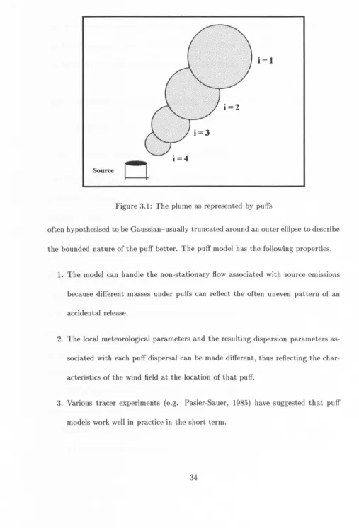
Figure 3.1: The plume as represented by puffs

often hypothesised to be Gaussian-usually truncated around an outer ellipse to describe

the bounded nature of the puff better. The puff model has the following properties.

1. The model can handle the non-stationary flow associated with source emissions

because different masses under puffs can reflect the often uneven pattern of an

accidental release.

2. The local meteorological parameters and the resulting dispersion parameters as

-sociated with each puff dispersal can be made different, thus reflecting the char

-acteristics of the wind field at the location of that puff.

3. Various tracer experiments (e.g. Pasler-Sauer, 1985) have suggested that puff

(47)

Because of these properties, a Bayesian model based on generalisation of the puff model has been adopted both to combine the puff model with expert judgements and monitor-ing data, and to provide an evaluation of the uncertainty associated with the forecasts.

3.4 A Statistical Forecasting Model based on RIMPUFF

Model

3.4.1 General Characteristics of RIMPUFF

The Rlso-Mesoscale PUFF-Model (RIMPUFF) is a Gaussian puff dispersion model developed at Riso in Denmark (see Mikkelsen et al., 1984 and Thykier-Nielsen

&

Mikkelsen, 1991). It is a fast operational computer code suitable for real-time sim-ulation of hazards from radioactivity released to the atmosphere. It has recently been adopted for inclusion into many decision support systems including RODOS.

RIMPUFF consists of an algorithm that models a continuous release by a series of consecutively released puffs. At each time step the model advects and diffuses the individual puffs in accordance with local meteorological parameter values. The rela-tionship between the movement and expansion of a puff and the local input parameters is extremely complex and non-linear. Concurrently, the model also monitors the re-sulting concentrations in selected grid points. The local meteorological parameters are organised in subprograms which can be readily changed or modified according to the needs and opportunities in the actual model situations.

(48)

with specific release rates in the specified grid. The individual puffs are advected by the wind field. RIMPUFF calculates the locations of puffs on the specified grid by computing their movements during finite time steps, using an interpolated wind field which is based on data from the wind measurement stations.

To compute the growth of the puffs, it is necessary to have simultaneous specifica-tions of the turbulence and/or the atmospheric stability. Once the advection and size of all puffs have been calculated, updated grid concentrations are obtained at each grid point summing up all the contributions from the puffs in the grid.

3.4.2 Stochastic Modification of the RIMPUFF

Smith

&

French (1993) have made use of the RIMPUFF model. The dispersion of time-dependent atmospheric plume is described by a sequence of directly released puffs whose superposition pattern approximates the concentration distribution of a contin-uous plume. The puffs are indexed such that puff i is released at time t

=

i. As-sume that the mass under puff i is Q(i). i.e. Q(i) is an uncertain quantity which represents the total number of contaminated particles under the ith puff. We define Qt = (Q(l), ... , Q(t))T which approximates the release profile of the source term. Stan-dard priors are used on the shape of the time profile (the time series) of the release. Such priors can model any uncertainty about the mass released and its duration. This gives a prior mean. Also we can encode "smoothness" in the release profile through the covariances between the Q (i) 'so

(49)

83 the vertical is given by the product Ft(i, s)Q(i). The stochastic multiplier Ft(i, s) determines how that emission is distributed over space and time. It is a proportion of the total contaminated particles under the ith puff at site s and time

t.

Typically Ft(i, s) is a complicated deterministic function of parameters, themselves calculated from uncertain meteorological inputs. For example, one of the simplest of such dispersal models is a Gaussian puff (see Pasler-Sauer, 1985), which sets

(3.1)

where (u(I), u(2)) is a wind velocity vector possibly depending on

t,

and h is the height of the emission. The radial growth of puffs during dispersion as a result of "internal turbulence" is described by the parameters

(O't(1),O't(2))

and

O't(3)

which denote puff sizes in horizontal and vertical directions respectively. These last param-eters relating to the diffusion are in part functions of meteorological data such as low frequency fluctuations in wind direction. The parameters of F_t(i, s) are calculated in rather complicated ways to take account of heterogeneity in the system. The function Ft(i, s) is often truncated and set to zero for

s

lying outside a contour with parameters

(O't(1)

=

0';(I),O't(2)

=

0';(2), O't(3)

=

0';(3))

(say). This explains why only a certain small number of puffs lie over a site s at any time.

(50)

• Relating an observation to puffs.

Instantaneous concentrations at monitoring sites are linear functions of Qt. Let Y{t, s) denote an observation taken under some overlapping puffs at time t at location

s.

Here Y

(t, s)

represents the total number of contaminated particles at (t, s). Now Y(t, s), the concentration of contamination, is simply the sum of concentrations of all puffs where the ith puff contributes a proportion Ft (i, 8) of its total mass

Q(i).

Thus Y(t,

8)

will be a linear function of the combinations of masses

Q(i)s.

In practice, because puffs are typically bounded, it is found that for many disper-sion models and scenarios that arise, only a few number of puffs will contribute to contamination at a given detector site at time t. This number of related puffs will be determined by the physical dispersion model. In terms of our formulation, it is implied that all but a few of the multipliers F_t(i,8) will be non-zero at a fixed point

(t,8)

• It is possible to use analogues of Bayesian DLM algorithms to assimilate a time series of monitoring data whose states are the uncertain masses.

In our application Y(t, s) will be a noisy function of the true contamination O(t, s) at site 8 at time t originating from Q(l), ... , Q(t). In practice the dispersal of the contaminated material is patchy (see Smith & French, 1993), and this needs to be modelled stochastically as

t

O(t, s)

=

E

Ft{i,

s)Q(i)

+

f{t, 8)

i=1

(51)

vari-ance U(t, a), and £(t, sd, £(t, S2) are independent for sites SI, S2. As a simple process (Y(t,s)l9(t,s)) is defined to have a Gaussian distribution with mean 9(t,s) and a fixed

variance V(t, s) where V(t, s) is assumed known and represents the "observation and modelling" error. Assume that Y(t, s) is independent of all other variables in the system given 9(t, s) then

Y(t,s)19(t,s)) '" N[9(t,s), V(t,s)] (3.2)

The methods can be generalised to assimilate non-normal data (see Chapter 8). The general observation process where Y(t, s) is a vector of observations taken at time

t

at a selection of sites s is discussed later in Subsection 3.6.1.1.

Now, conditioning on everything else other than masses, the model provides elegant algorithms to: update distributions of the source term in time; predict contamination over space and time; and hence to obtain predictive distributions of data and also to admit data assimilation.

However, in practice many of the variables coditioned on will be unknown. For example, we may be uncertain about a parameter like the release height and we know that this parameter has a significant effect on the multipliers.

(52)

3.4.3 Modelling Uncertainties about Meteorological Input and the

Dispersion Model

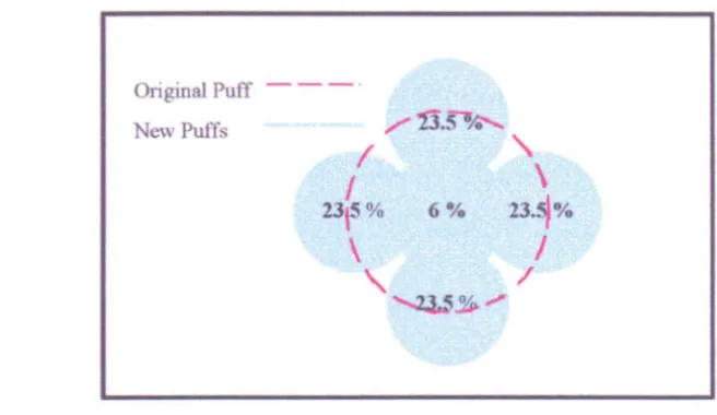
When the dispersal model is inadequate and its meteorological inputs are inaccurate then the statistical model described above cannot be expected to work well in practice. Fortunately, however, a splitting feature called pentification which is coded within the deterministic models of RIMPUFF can be adapted to manage, indirectly, much of the uncertainty indicated above.

(53)

Original Puff

[image:53.534.94.422.46.236.2]

New Puffs

Figure 3.2: Puff pentification

algorithm deterministic. In the statistical model we allow for the possibility that reality

may be better modelled by a different percentage split, i.e. that one or more puffs may

receive more than their expected share of the contaminant, and that correspondingly

others may receive less. As monitoring data are assimilated, the model may learn that

such an asymmetric pentification would be more appropriate, and it will adjust the

masses of contaminant in each puff accordingly. One effect of this is to shift the overall

plume somewhat to take account of such things as misspecification of the wind field

and dispersion model.

Explicitly the sibling vector of the children of the i th puff/ puff fragment Q (i)

(Q( i, 1), ... ,

Q(

i, 5)) can be expressed as

Q (i) = OtQ (i)

+

w ( i) (3.3)

where

(54)

and

w(i) = (w(i,1), ... ,w(i,5))

is a system error chosen to conserve mass i.e.

Ej=l

w(i,j) = 0 with Var[w(i,j)] =

W.

One simple example sets w{i) '" N[O, W*], where W* is a covariance matrix of shape

1 _-41 _-41 _{-4 -4}1 1 1 ₁ 1 1 1

-4 -4 -4 -4

W*= 1 1 ₁ 1 1 _W _(3.4)

-4 -4 -4 -4:

1 1 1 ₁ 1

-4 -4 -4 -4

1 1 1 1 ₁ -4 -4 -4: -4

Now equations (3.2), (3.3) and (3.4) specify a simple linear stochastic system. This system is rich enough to exhibit sensible learning procedures for a variety of plausible scenarios. Also it faithfully mirrors in its structure a dispersal model that a physicist understands. It requires as prior inputs only:

i)

The first two moments of the mass under each puff on emission.

ii)

A measurement error variance.

iii) A variance parameter to define the stochastic pentification.

3.5 Model Adaptation

(55)

00

i

=l

i=

2

[image:55.530.52.491.75.492.2]

i=

3

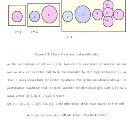
Figure 3.3: Plume trajectory and pentification

on the pentification are set as in (3.4). Consider the case where we observe

contam-ination at a site predicted only to be contaminated by the fragment labelled (1, 5).

Then it easily shown from the related equations defining the statistical model and the

pentification covariance that the joint Gaussian distribution of (Q(I), Q(I), Y) has a

mean vector (q(l),

o:

q(l), la5q(1)) where

Q(l)

=

(Q(l, 1), ... , Q(l, 5)), q(l) is the prior mean of the mass under the first puff,

0:

=

(all a2, a3, <1'4, 0'5)

=

(0.235,0.235,0.235,0.235,0.058)

and

I

= Ft (" s) with Ft (., s) as defined in (3.1). The covariance matrix of (Q(l), Q(l), Y)

is given in a block matrix form as

S

o:

T

S la5 S

o:TS C c

(56)

where S is the prior variance of the mass Q(l) and C = {Cij } where 1~i=j~5

if-j

where

W

is the variance of the system error in the first pentification.

c = f(C_{15 , ••• ,}C55

f

where Cij is defined above, and d = PC55

+

V, with V the

observational variance of Y conditional on Q(l, 5).

Now, using the usual normal theory, it is easy to derive the revised distribution of q(l) given Y, which is a multivariate normal with mean vector

qt(1)

and covariance matrix

Qt(1)

where

(3.5) and

qt(1)

=

(it(I, 1), ...

,qt(1,5))T

where for 1 ~ j ~ 5

(3.6)

where

et(5)

=

7 -

a5q(1) (3.7)

(1') f[aj a5S - 1/4W] J' -J. 5

a ,) = J2[a~S

+

W

+

V/

J2]'

f (3.8)

a(1,5)=

7-

[1-

a~s+%':v/J2l

(3.9)

where

ajq(l) is the expected contamination under puff (I,j) before observing y.

et(5)

is the difference between the naive estimate of

q(l,

5) using y and its prior expected value.

(57)

1. The adaptation of the fragment (1, 5) associated with the observation y pulls the mean towards the naive estimate y

I

I.

2. The larger the uncertainty in the source (8) and the uncertainty in the pentifica-tion (W) relative to the observational error variance V, the greater the adaptation towards the naive data based estimate.

3. The adaptation of beliefs associated with sibling fragments is interesting. Adap-tation of the mean towards or away from the naive estimate

yl I

of q(1, 5) will depend on whether the ratio 81W is large or small. Thus we adjust towards the naive estimate if the source uncertainty is large (assuming this has been mis-estimated) and away from the naive estimate if the source reading is accurate. In the later case, if more contamination than expected has been observed under puff (1, 5), then less must exist under puffs (1, j), 1 ~ j ~ 4. This illustrates the critical role of the settings of prior variances on the subsequent management of uncertainty.

To adjust beliefs about the source emission quantity Q(1), notice that, given y, this has a Gaussian distribution with mean (It(l) and variance

Qt(1)

where for

la5

#-

0

and

1 [

VIP

+

W

1 a(1)

=

la5

1 -

a~8

+

W

+

VI

J2 .

(58)

3.6 A Dynamic Fragmenting Puff Model

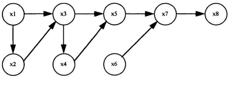
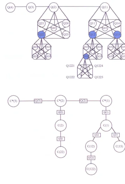
Although we have argued that the above statistical model might be appropriate from a theoretical standpoint, there is a practical requirement that we have to meet. The covariance matrices within the model can become very large in dimension, and compu-tational efficiency thus declines dramatically. Fortunately, this fragmenting puff model can be restructured as a dynamic junction tree, (see Chapter 7). In fact Smith et aI., (1995) address this problem. They have shown how the Bayesian propagation algorithms (Lauritzen & Speigelhalter, 1988) can be modified when the trees evolve dynamically. Their methodology is defined and illustrated within a stochastic version of a fragmenting puff model. In this section we describe briefly their methodology, starting with a notation and some distributional assumptions which we will follow in later chapters.

3.6.1 Model Description

With reference to the puff splitting scheme of section (3.4), fragments arising directly from another puff or puff fragments will be called children of a parent puff/ puff frag-ment. In RIMPUFF each parent puff has five children and is said to be pentificate.

Let m(t, I) = m(t, It, ... , Ik) be the puff fragment which is the ILh child of the

ILt:l

child, ... , of the lih child of the puff released at time t. In RIMPUFF 1

5

Ii

5

5, lSi

5

k. The index k relates to the number of fragmentations that have taken place before fragment m(t, I) appears. Let:

(59)

q(l) denote the vector of true masses under the set of the children of m(t, I). Q(I) = (Q(I), q(I))T

3.6.1.1 The Observation Process

Let QT be the vector of masses of all puffs and puff fragments emitted on or before time T. Let Y(t, s) denote a vector of observations taken at time t at a selection of sites s. Assume that Y(t, s)18(t, s) is independent of all other variables in the system. Here 8(t, s) can be interpreted as a random vector relating to the actual mass at time t on site s unconfounded with the observational errors in Y(t, s). As a simple process, Y(t, s)18(t, s) is defined as having a Gaussian distribution with mean 8(t, s) and a fixed covariance matrix V. As explained in Section (3.4), an important feature of puff models is that at all points (t, s) of the observation grid, 8(t, s) can be written as

8(t, s) = F(t, s)Qt

+

€(t, s).

Issues in the Bayesian forecasting of dispersal after a nuclear accident

University of Warwick institutional repository:

http://go.warwick.ac.uk/wrap

A Thesis Submitted for the Degree of PhD at the University of Warwick

http://go.warwick.ac.uk/wrap/73485

This thesis is made available online and is protected by original copyright.

Please scroll down to view the document itself.

ISSUES

THE BAYESIAN FORECASTING

of

DISPERSAL AFTER A NUCLEAR ACCIDENT

Ali S. Gargoum

Contents

List of Figures

0'2] .

List of Tables

Chapter

1

Introd uction

1.1 Background

ASY

CSY

ESY

,r

,r

"

1.2 Aims

1.3 Outline of the Thesis

Chapter

2

Dynamic Linear Models: A Brief

Review

2.1 Introduction

2.2 Bayesian Forecasting and Dynamic Models

lit

t -

"'t.

2.3 The Univariate DLM

2.3.1 Definition

t

t

Yt]

Yt

t.

N[mo, Co], where mo is the prior expectation for

2.3.2 Model Updating

Wh

t,

(8

ID

-d

+

(YtID

E[YtIDt-tl

-

it

Var[YtID

+

\.'t.

=

t

+

2.3.3 Forecast Distributions

+

t

(a)

+

=

=

t,

2.4 The Discounting Concept

=

<

<

=

=

=

¥

=

2.5 Dynamic Estimation of Variance

_{tIAt, Dt-dlDtl}