1
ECE-320 Lab 8:
Utilizing a dsPIC30F6015 to control the speed of a wheel
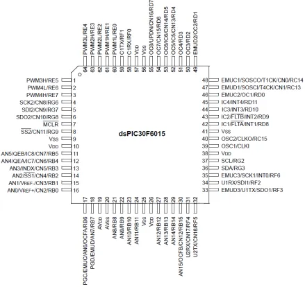
[image:1.612.83.522.262.676.2]Overview: In this lab we will utilize the dsPIC30F6015 to implement a PID controller to control the speed of a wheel. Most of the initial code will be given to you (see the class website), and you will have to modify the code as you go on. One of the things you will discover is that you often need to be aware of limitations of both hardware and software when you try to implement a controller. The dsPIC30F6015 has been mounted on a carrier board that allows us to communicate with a terminal (your laptop) via a USB cable. In what follows you will need to make reference to the pin out of the dsPIC30F6015 (shown in Figure 1) and the corresponding pins on the carrier (shown in Figure 2)
2 Figure 2. dsPIC30F6015 carrier. Note that the pin numbers are not consecutive.
Part A (Copying the initial files)
3 Part B (Putting it all together)
Now we are ready to start. Note that at some point in the following process you may need to let the system download firmware. Be sure you have selected the correct device (or it will do this twice).
Start MPLAB X IDE (not IPE)
Select File, then New Project (the screen should default to Mocrochip Embedded and Standalone Project)
Click on Next
In the Select Device section, select the following:
Family: 16-bit DSCs (dsPIC30) Device: dsPIC30F6015
Click on Next
In the Select Tool section, select PICkit3 Click on Next
In the Select Compiler section, select XC16 Click on Next
In the Select Project Name and Folder section, choose a name and project location
Click on Finish
Make sure the file lab8.c is in the Project folder. Right click on Source Files, then on Add Existing Item, then select lab8.c
4 You should build (compile) the existing program, download it to the dsPIC, and run it. You should see a sequence of numbers on your screen (the secure CRT screen). These correspond to sample times.
If you see the following message
You are trying to change protected boot and secure memory. In order to do this you must select the "Boot, Secure and General Segments" option on the debug tool Secure Segment properties page. Failed to program device
Then
• Right Click on the Project Name and select Properties • Under Categories in the left panel, click on PICkit3
• Under Option categories at the top, select Secure Segment • On the right select Boot, Secure, and General Segments • Then select ok at the bottom.
Your program should now compile.
Part C: Reading in the sensor transducer
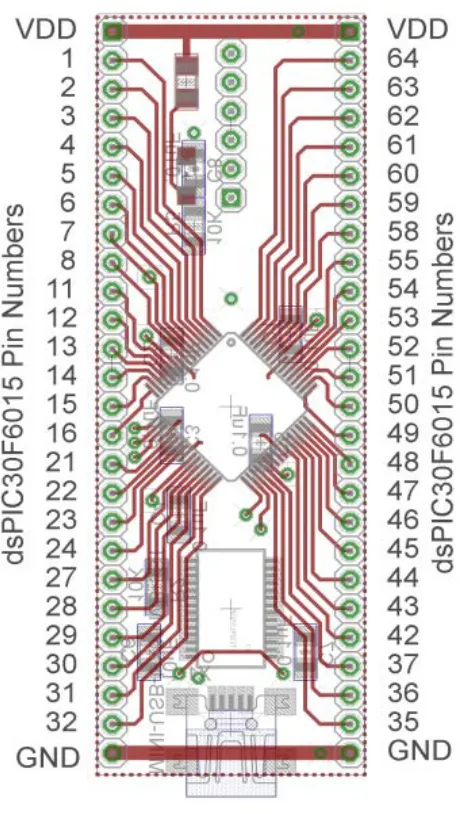
[image:4.612.170.442.525.603.2]In order to determine how fast the motor is spinning, we will need to use the QEI interface. The sensor is connected to the center of the wheel, and the other end of the sensor plugs into the breadboard. The pins for the interface are shown in Figure 3. You need to connect this interface to +5 volts (red ), ground (blue), and the QEA Channel A input (pin 12), and the QEA Channel B input (pin 11).
5 Part D (Reading in an A/D value)
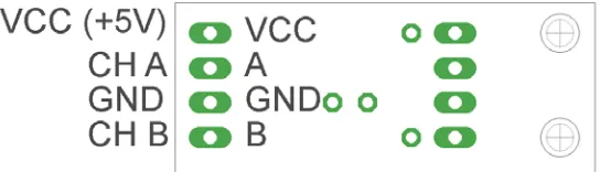
Now we want to be able to connect a potentiometer as shown in Figure 4 so we can have a variable reference. The software is currently set up for A/D input on AN3/RB3 (pin 13). You will need to do the following things:
• Connect the potentiometer as shown below • Set the appropriate TRIS bits for an input signal
[image:5.612.236.406.245.399.2]Note that this is the same set-up as was used in Lab7.
Figure 4. Connecting the potentiometer Part E: Connecting the power entry
Plug in both the 5 volt (green) and 12 volt (red) power supplies, as shown in Figure 5. Do not turn on the supplies yet (the LEDs should be off) .
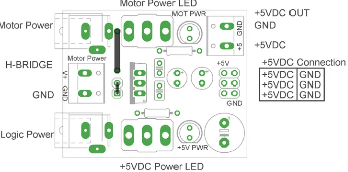
[image:5.612.135.480.520.691.2]6 Part F: Connecting the H Bridge
[image:6.612.58.518.167.330.2]Plug in the H-bridge, shown in Figure 6. You are going to need access to the different pins, so be sure it is located in a place you can easily get wires to.
Figure 6. H Bridge connections
Starting on the left, connect the ground and +5 volt supplies. Next, connect IN1 to RE6 (pin 2) and IN2 to RE7 (pin 3). (Note that if the motor speed is negative you may want to reverse these connections.) Finally connect PWM to PWM 3 high (pin 1).
Starting on the right, connect (with the twisted wires) the 12 volt power from the power entry module to the 12 volt input. Be sure to connect ground to ground and +12 to +12. Next, connect M1 and M2 (using the twisted wires from the wheel) to the motor input.
At this point all of your wiring should be done. You should check it over before you go on.
Two important things to keep in mind as you do the remainder of this lab:
• Use the red switch to shut off power to the motor. Sometimes stopping the dsPIC does not stop the motor, in which case you will need to use the switch.
7 For this lab, it is probably much easier to use the debugging features in MPLABX
Click here to compile and download to PIC
Click here to pause Click here to exit (stop)
Click here to reset
8 PART G: Determining Initial Scaling
We need a new program now to control the motor. You will modify lab8.c for the remainder of this lab. Now we will start to determine some of our parameters. Turn on the power to the motor (the red LED should turn on) and open SecureCRT. When the program starts to run, the output to the screen is the current time, the value read from the pot, the dutycycle, and the speed of the wheel in radians/sec.
With the system at rest start the program and slowly turn the pot so the motor is spinning. Turn the pot so the motor is spinning at less than or equal to 30 rad/sec. Let the motor come to a reasonably steady value (it will likely keep getting faster). Wait until the motor speed is fairly constant and the input reading from the pot is also fairly constant. Record the reading from the pot and the speed of the motor. Do this for three different positions of the pot where the steady state speed is less than 80 rad/sec. (Note that it is likely to be easiest to use the session log file than look at the screen output.)
We now want to determine the proportionality constant between the A/D value read from the pot and the motor speed in rad/sec. Compute the three scaling factors and average them (mine was approximately 0.170).
Change the parameter AD_scale (in your code) to this value. Run the system again at various input values. It may take a while for the system to reach steady state. Compare your reference input to the actual output. They should be fairly close for some speeds but they will not be exact. For other speeds they may be off by a significant amount. This is open loop control.
PART H: Proportional Control
We now want to start with our first control scheme, proportional control. You will need to declare the variable kp as a double (at the top of the main routine). Outside of the main loop set kp = 1.0, and inside the main loop, after both the speed and reference input are determined, compute the error as error = R-speed. Here R is the reference input and speed is the measured output speed of the wheel in
rad/sec. The control effort is then proportional to this error, so u = kp *error.
Recompile and download the code onto the microcontroller. Now start the system again. Move the pot to a number of different set points, and wait until the system comes to steady state. Most likely the steady state value will be approximately one half of the set point.
Stop the system and change the value of kp to 5, and then to 10. (Be sure to recompile and download after each time). Run the system again for each value of kp. You should notice that the steady state error gets smaller as kp increases.
PART I: Limiting the slope of the control effort
9 Starring with kp = 10.0, start the system and turn the pot (setting the reference input) as quickly as you can (but don’t worry about turning it all the way). You hear strange sounds from the motor like it is starting and stopping (or worse).
What we need to do in this case is limit the rate at which we allow the control signal to change. At the top of the code there is a constant MAX_DELTA_U which indicates the maximum change in control effort u from one time step to the next. This constant is going to need to be changed (but we will get to that). Declare a new (double) variable last_u, and set this variable equal to zero outside the main loop. Inside the main loop, add statements to the code that do not allow the control effort to increase by more than its current value + the maximum allowed increment. Insert this limit on the control effort after converting to a pwm signal but before we check that the control effort is not too large. Also be sure to update the value of last_u. However, do not update this value until the other statements in the code that insure that the value of u is within acceptable limits. Finally, you will need to set the value for
MAX_DELTA_U. I would start at around 1000, and change this as necessary. Try to get this value as large as possible. Run your code and try to change the pot (the reference input) as quickly as possible. Once you think your values are ok, set kp=100.0 and be sure your system runs acceptably (the motor does not shut off and on).
PART J: Proportional controllers with large gains
Make sure kp is set to 100 for this part. Compile the code if you need to and start it running. Vary the reference signal to a few set points (such as 30 rad/sec, 60 rad/sec, and 90 rad/sec) and allow the system to try and reach steady state at each of these set points. You should notice that the speed of the wheel varies significantly from the reference point. Part of this is due to the fact that the motor is only capable of one direction, but a larger part is due to the fact that small errors are amplified (by 100) and this causes the motor to continually oscillate.
PART K: Integral control
Recall that using a prefilter to control steady state error can sometimes be problematic since the prefilter is outside the feedback loop. An alternative, and generally better, solution is to include some form of integral control. Recall that an integral controller has the form
1 = ) ( ) ) ( 1 ( i c
k U z
z z z G E − = −
Rearranging this we get
1
U(z) ( ) ( )
iE z U z
k = −z−
In the time-domain this becomes
( ) ( ) ( 1)
ie n u n u
10 Since we want the control effort as our output, we will write this as
( ) (n 1) i ( )n u n =u − +k e
If we assume the initial control effort is zero, we can write this as follows:
1
(1) (0) (1)
(2) (2) (1) [ (2) (1)]
(3) (3) (
(1
2) [ (3) (2) e(1)]
( ) ) ( ) i i i i i i n i k
e u k e
u k
u
e u k e e
u k e u k e e
u n k e k
k = + = = + = + = + = = = + +
∑
Hence to implement the integral control, we need to sum the error terms and then scale them by ki. Declare two new (double) variables Isum and ki. Set the initial value of Isum to zero outside the main loop. Within the main loop update the error summation using something like Isum = Isum + error. Within the main loop implement a PI controller as follows:
u = kp*error + ki*Isum;
Set kp = 0.0 and ki = 0.1. Modify the print statement at the end of your code so the value of Isum is also printed out. Recompile and download your code. Start the system and set the reference signal to a few reference points (30, 60, 90 rad/sec, for example), and let the system run for a while. Your system will probably exhibit some pretty strange behavior on its way to the correct steady state value (it will bounce around the steady state value due to sampling). Look at what is happening to the value of Isum during this strange behavior.
PART L: Integrator problems
The first problem we need to fix is that our motor is only spinning in one direction. When Isum
becomes large and negative, we would expect the motor to spin in the other direction, but it can’t. One way to minimize this effect is to check to be sure that the value of Isum is greater than or equal to zero. Modify your code to do this, recompile, and run it again.
The second problem we have is called integrator windup. Basically, the accumulated error is becoming too large and causes the system to overshoot, and then undershoot. One way to fix this is to limit the value of Isum to a maximum value. There is a defined variable at the beginning of the code
11 someplace to start looking). Do not move on until you have what you think is a reasonable value of MAX_ISUM and your code seems to be working. Note that you will still have some oscillations, and that to get to a large steady state value MAX_ISUM will need to be fairly large.
PART M: Including a derivative term
Finally we need to include a derivative term to implement a full PID controller. You will need to define three new (double) variables, kd, Derror, and last_error. Outside of the main loop set last_error equal to zero and set kd equal to 0.01.
Inside the main loop include the lines
Derror = error-last-error; last_error = error;
Finally, to implement the full PID controller define the control error u to be u = kp*error+ki*Isum+kd*Derror;
Compile and download your code, and try a few reference points. Your system may still oscillate, but we can work on that soon.
PART N: Designing a PID controller
At this point, we want to hardcode the value of the reference signal so the step response will start as soon as we turn on the system. With the system at rest, twist the pot to a reference value and look at the step response. Try to get to a reference point greater than 90 rad/sec.
A general plan for designing a PID controller using a trial and error method (we have no model for the plant) is the following:
• First, set ki = kd = 0, and try to get a good response for a step input using only kp.
• Next, adjust ki to get a good steady state error. Since the integral control tends to slow the system down, don’t make this any larger than you need to. However, you may need to also change MAX_ISUM to get a good response.
• Finally, adjust kd to speed up the response.
Once you have a good design, you need to log your data so you can make a Matlab plot. If you have saved your data in a file named (for example) play3.log, then in Matlab type
data = load(‘play3.log’);
t = data(:,1);
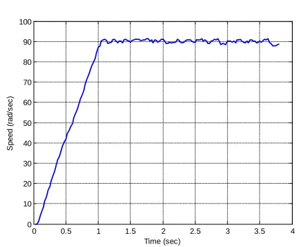
12 You may have to edit your files to make nice plots (like using t = t-t(1)). Be sure to include labels on your axes. The plot I have for one of my results is shown in Figure 7.
Design PID controllers to meet the specifications shown below.Include a Matlab generated figure of your step response results in your memo, and be sure to include both the sampling interval and the values of kp, ki, and kd. Also attach your final code to your e-mail.
(i) For a sampling interval of T = 0.025 sec (the default) our design criteria is a settling time of less than or equal to 1.2 seconds, and a percent overshoot less than 10%.
[image:12.612.78.508.257.616.2](ii) For a sampling time of 0.1 sec, our design criteria is a settling time of less than or equal to 4.0 seconds, and a percent overshoot less than 10%.
Figure 7: Step response for system with T = 0.025 seconds. I am not telling you my parameter values. Finally, I would appreciate any comments you may have on this lab, and how to improve it. Also, do you think it was useful and we should do more labs like this in the future or not?
0 0.5 1 1.5 2 2.5 3 3.5 4 0
10 20 30 40 50 60 70 80 90 100
S
peed (
rad/
s
ec
)