1 Comparing Spatial Patterns
1 2
Jed A. Long1,* and Colin Robertson2 3
4
1School of Geography & Sustainable Development, University of St Andrews 5
2Department of Geography & Environmental Studies, Wilfrid Laurier University 6
7
*Corresponding Author Email: [email protected] 8
9 10
Comparing Spatial Patterns 11
Keywords: maps, correlation, scale, bivariate, comparison, model assessment, spatial process 12
13
Abstract 14
The comparison of spatial patterns is a fundamental task in geography and quantitative spatial 15
modelling. With the growth of data being collected with a geospatial element we are witnessing 16
an increased interest in analyses requiring spatial pattern comparisons (e.g., model assessment, 17
change analysis). In this paper we review quantitative techniques for comparing spatial 18
patterns, examining key methodological approaches developed both within and beyond the 19
field of geography. We highlight the key challenges using examples from widely known 20
datasets from the spatial analysis literature. Through these examples we identify a problematic 21
dichotomy between spatial pattern and process – a widespread issue in the age of big geospatial 22
data. Further, we identify the role of complex topology, the interdependence of spatial 23
configuration and composition, and spatial scale as key (research) challenges. Several areas 24
ripe for geographic research are discussed to establish a consolidated research agenda for 25
spatial pattern comparison grounded in quantitative geography. Hierarchical scaling and the 26
modifiable areal unit problem are highlighted as ideas which can be exploited to identify pattern 27
similarities across spatial and temporal scales. Increased use of ‘time-aware’ comparisons of 28
spatial processes are suggested, which properly account for spatial evolution and pattern 29
formation. Simulation-based inference is identified as particularly promising for integrating 30
spatial pattern comparison into existing modelling frameworks. To date, the literature on spatial 31
pattern comparison has been fragmented and we hope this work will provide a basis for others 32
to build on in future studies. 33
2 35
Word Count Original (Intro to Conc): 7346 36
Word Count Revised (Intro to Conc): 6132 37
3 1. Introduction
40
The comparison of maps is a fundamental part of how geographers try to understand 41
the world. Quantifying spatial distributions and patterns, and comparing across regions or over 42
time is central to many types of geographical research and applications. To illustrate, Figure 1 43
presents two maps from the recent Intergovernmental Panel on Climate Change (IPCC) 44
Synthesis Report (IPCC, 2014) which shows recorded surface temperature change (1986-2005) 45
and projected changes (2081-2100). We are confronted with two simultaneous map comparison 46
tasks. First, we make comparisons locally within a map, noticing spatial differentiation within 47
both observed and projected temperature regimes – noting in particular the rapid warming in 48
polar regions. Second, we compare the maps globally, recognizing large magnitude shifts in 49
temperature across most continents in the projected scenario compared to the period of 50
observed temperature changes. In making these interpretations broadly, we mask uncertainties 51
associated with more precise questions of change, such as which populations are likely to be 52
most impacted by increasing temperatures, where should conservation resources be allocated, 53
are countries in the global North more impacted than the global South, were the data collected 54
equally in all regions, and countless other geographic questions. These maps are included in 55
the IPCC report designed as guidelines for policy and decision-makers. The recognition and 56
quantification of spatial change through comparison of spatial patterns, both globally and 57
locally, represents an important and under-recognized research area for geography which we 58
aim to review, critique, and contextualize. 59
<Figure 1 here > 60
Many of the origins for studying changes and differences in spatial patterns arose during 61
geography’s quantitative revolution. Today the sheer volume of geographically referenced data 62
is providing new opportunities for geographers to compare spatial patterns across space, and 63
time. Recent geographical data-intensive research streams include geocomputation (Openshaw 64
& Abrahart, 1996); geospatial big data (Li et al., 2016), human dynamics (Shaw, Tsou, & Ye, 65
2016), and geographic data mining (Miller & Han, 2009). Long-term archives of satellite 66
imagery, crowdsourced geospatial databases, and open data portals are now being developed 67
and maintained for a variety of subject areas. Despite the amount of data-intensive geographic 68
research taking place, geographers have not consolidated methods and models for performing 69
spatial pattern comparisons which facilitate replication, identification of broader trends and 70
underlying spatial process dynamics, and local anomalies. 71
In this paper we review existing quantitative techniques for comparing spatial patterns 72
4 associated with spatial patterns before moving on to a review of selected techniques, and 74
provide illustrative examples that highlight strengths and shortcomings of current methods. We 75
conclude with some thoughts on the research needs for spatial pattern comparison (SPC) in 76
geography today. In doing so we hope to provide some coherency and unity to the SPC research 77
which is fractured across fields, and identify research opportunities for geographers interested 78
in quantitative spatial analysis. 79
2. Characteristics of Spatial Pattern Comparison Problems 80
2.1 Characteristics of spatial patterns 81
As geographers, we typically ascribe meaning to spatial patterns as the outcomes of multiple 82
and interacting spatial processes (O’Sullivan & Unwin, 2010). Isolation of processes 83
themselves outside of laboratory or simulation environments is impossible at most 84
geographically-relevant scales, so while detecting change in a spatial pattern can reveal 85
changes in underlying processes, it is not sufficient to reveal those dynamics. Complicating 86
matters, pattern itself acts on and perturbs the processes generating patterns (Turner, 1989). 87
Even the term spatial pattern can itself imply multiple and conflicting phenomena. Here we 88
use a definition (see Box 1 for a glossary of terms and definitions that will be used throughout) 89
based on that of Dale (2000), that a spatial pattern is the scale-dependent predictability of the 90
physical arrangement of observations. 91
< Box 1 (Glossary) Here > 92
2.2 Spatial representation 93
Spatial data are abstractions of reality, with ‘features’ (i.e., the things we demarcate, 94
categorize, and label in the world) represented by points, lines, polygons (areas), and 95
continuous spatial lattices (irregular or regular) in a digital mapped form. These are the core 96
spatial data types available in a geographic information system (GIS) and there exists relatively 97
few other ways to represent spatial phenomenon in a GIS (Roberts & Robertson, 2016). The 98
representation of complex physical and societal characteristics (in spatial data) influences how 99
feature or attribute data can be characterized, visualized and subsequently analysed (Miller & 100
Wentz, 2003). Nearly all examples of SPC that will be discussed in this paper represent what 101
can be termed ‘diagonal’ comparisons (referring to a matrix of spatial data types; e.g., see 102
O’Sullivan & Unwin, 2010, p. p26), that is, for example, point-point and lattice-lattice 103
comparisons. 104
2.3 Statistical properties 105
Methods for SPC can also be characterised as being entity-based or attribute-based. 106
5 limited to spatial comparisons of points, lines, and polygons (areas). Attribute-based 108
comparisons simultaneously consider patterns associated with both location and attributes. 109
With attribute-based comparisons, whether the attribute type is continuous or categorical also 110
impacts how a spatial comparison is framed. Most attribute-based comparisons are associated 111
with fixed spatial arrangements (i.e., the locations are the same in both maps), but this need not 112
be the case. 113
SPC methods can further be broken down along dimensions of spatial pattern that they 114
compare, whether local or global aspects of pattern, or the abundance (composition) or 115
arrangement (configuration) of mapped values (Figure 2). At the global level, SPC can be 116
undertaken by either computing a single univariate measure, such as Moran’s I index of spatial 117
autocorrelation (Cliff & Ord, 1973), individually on each map; or by computing a bivariate 118
measure that simultaneously compares values in two maps. In the first case, only a coarse 119
understanding of spatial pattern change can be inferred, for example a change from complete 120
spatial randomness to spatially clustered. One of the challenges with the former approach, is 121
that both local-to-global scaling and composition vs configuration are highly interdependent 122
concepts, posing challenges for robust statistical significance testing. Some specific measures 123
have been proposed for disentangling global and local spatial structure such as the Oi statistic
124
(Ord & Getis, 2001), however these have not been widely adopted. Similarly, composition and 125
configuration are also interdependent, and several authors have highlight the need to compare 126
measures of spatial configuration only in the context of spatial composition (Cushman, 127
McGarigal, & Neel, 2008; Long, Nelson, & Wulder, 2010; Remmel & Csillag, 2003). In 128
bivariate comparison measures, these issues are partially overcome, as the distributional issues 129
associated with comparison are resolved by reduction of the parameter space to a single metric 130
(e.g., the root mean square error or the Kappa statistic). 131
2.4 Types of questions 132
Finally, SPC can be characterised as one of three types of question: change, similarity, 133
and association. Each type of SPC question can be specified in terms of the constraints and 134
variability in space, time, and theme of the patterns being investigated (Sinton 1978). Studies 135
of change involve cases where space and theme are fixed and time varies. The goal of change 136
analysis is often to identify whether change has occurred (globally), where such changes are 137
located (locally), and whether changes represent a significant change (Boots & Csillag, 2006; 138
Remmel & Csillag, 2003). Similarity questions involve situations where space is varied and 139
theme is fixed (time can be fixed or varying). Similarity tasks are prominent in the image 140
6 imagery (e.g., Yang & Newsam, 2013). Studies of associations involve cases where space is 142
fixed but theme varies (again time can be fixed or varying). Questions concerning spatial 143
associations are common in both the physical and social sciences (e.g., Austin et al., 2005; 144
Jones, Rendell, Pirotta, & Long, 2016). 145
A distinct and popular application for SPC is in spatial model assessment. Models that 146
produce mapped outputs can be compared to reference data to assess model fit, or across model 147
frameworks and parameterizations. Early examples of using SPC for model assessment include 148
Cliff (1970) and Sokal et al. (1983), who both characterized model outputs with spatial 149
autocorrelation statistics. Spatially explicit model assessment is critical as it can reveal patterns 150
in error structures not evident in error statistics (e.g., Plouffe, Robertson, & Chandrapala, 151
2015). SPC for model assessment, has seen more recent interest in the area of categorical spatial 152
data (e.g., land cover maps; Hagen-Zanker & Martens, 2008; Visser & de Nijs, 2006). 153
Examining the spatial pattern of model outputs as a complementary measure of model quality 154
underscores the importance of spatial pattern/process in environmental modelling (see Bennett 155
et al., 2013). 156
<Figure 2 here> 157
3. General approaches for Quantitative Spatial Pattern Comparison 158
3.1 Visual spatial pattern comparison 159
The human visual system excels at recognizing shapes and patterns. Our brains are able 160
to process information on shapes and patterns independently from context (Marr, 1985). Thus, 161
to date a large body of work on SPC has involved visual comparisons, and most commonly this 162
involves the presentation of maps side-by-side as a tool for visual SPC (see, for example, Figure 163
1 above). Comparing patterns in maps has led to some significant geographical insights, for 164
instance, Wegener’s work on continental drift theory was largely initiated by identifying 165
similar patterns in maps of the coastlines of Africa and South America (Wegener 1966). 166
However, comparing spatial patterns is visually challenging, as the human visual system is not 167
well adapted to judging spatial correspondence between two variables on side-by-side maps 168
and is more sensitive to the color classification scheme (e.g., Lloyd & Steinke, 1977; Steinke 169
& Lloyd, 1983). Moreover, MacEachren (1995, p. 403) suggests that we would expect visual 170
comparisons of maps to be more successful when changes are compositional (e.g., symbol size, 171
color) then with configuration changes (e.g., shape, and orientation). 172
Perception of patterns in maps is a function of our perceptual attention (i.e., where, and 173
for how long we look), also termed saliency. When comparing maps, cosaliency represents the 174
7 not correspond to salient features in individual maps (Jacobs, Goldman, & Shechtman, 2010). 176
Within the cartographic literature a number of techniques for enhancing visual map comparison 177
tasks have been developed (See Ch. 9 in MacEachren, 1995 for example). Many newer 178
techniques have abandoned side-by-side comparisons in favor of overlay techniques, and 179
implement tools such as translucents, swiping, and lenses (Lobo, Pietriga, & Appert, 2015). 180
However, it is widely acknowledged that visual SPC is challenging, most notably in assessing 181
changes in spatial configuration, a problem that continues to hinder both visual and quantitative 182
assessments of SPC. 183
3.2 Comparing spatial point patterns 184
Tobler (1965) studied the correspondence between pairwise point patterns of the 185
locations of birth for a sample of married couples in Japan using a comparison measure which 186
he termed the affine correlation statistic. The approach was innovative in terms of its attempt 187
to draw on Pearsons correlation coefficient, but was limited to cases where two patterns had 188
the same number of points and the points are naturally paired. Ecologists were early adopters 189
of statistical methodologies for comparing bivariate point patterns, notably the work of 190
Anderson (1992) who drew on seminal methods from Diggle (2003), to compare one point 191
pattern to another with the bivariate extension of the K-function. 192
In biology, tight coupling of spatial and physical factors that drive the control and 193
function of cellular functions and processes demands rigorous methods to detect differences in 194
pattern. Myers (2012) highlights the increasing need for quantitative approaches for SPC in 195
microscopy resulting from new forms of medical imaging data that are often used to derive 196
spatial point patterns. Many proposed approaches have bene tailored to specific biological 197
applications (e.g., Bell & Grunwald, 2004; Burguet & Andrey, 2014) however opportunities 198
exists for generalization to other, more complex, classes of spatial data. 199
3.3 Comparing line and polygon data 200
There are fewer methods available for comparative analysis of line and polygonal 201
pattern data. Within the geographical literature, line and polygonal spatial representations tend 202
to be treated as features rather than patterns, with emphasis of methods on the proximity and 203
orientation relations between pairs of objects, and summarizing such metrics over the dataset 204
provide a measure of global similarity. Maruca and Jacquez (2002) provide polygon 205
comparison statistics called area-based association measures, which essentially quantify the 206
degree of correspondence based on area overlap between two of polygon pattern datasets. 207
8 assessment, such as buffering a reference line and comparing the proportional overlap of a test 209
line (e.g., Goodchild & Hunter, 1997). 210
Graph analysis provides a large body of theory and methods for characterizing 211
networks, which is a common way to represent spatial line data in geographic applications. 212
These network representations can be compared through measures of including centrality, 213
connectivity, degree and others. However, often the geographical context is ignored to focus 214
on topological properties. The uptake of these methods in a spatial context has been greatest in 215
landscape research, examining structural (e.g. configurational) properties of a matrix of habitat 216
patches (i.e., nodes) and their spatial connectivity (i.e., edges) (Bunn, Urban, & Keitt, 2000; 217
Urban & Keitt, 2001; Urban, Minor, Treml, & Schick, 2009). Similarly, landscape ecologists 218
are interested in SPC of maps of land cover types, using indices of diversity, fractal dimension, 219
and shape (e.g., Mladenoff, White, Pastor, & Crow, 1993). However, these comparisons are 220
focused on comparing the measures of pattern in one map to another, rather than on bivariate 221
methods. Robertson et al. (2007) provide a comparison framework adapted from Sadahiro and 222
Umemura (2001) for studying temporal changes in spatial polygons which focuses on problems 223
where the spatial locations of polygons move through time (e.g., a forest fire). Here, changes 224
are characterized as events derived from topological and proximity relations of two polygon 225
patterns. 226
3.4 Comparing patterns in spatial lattices 227
There are many more methods for comparing patterns on spatial lattices, and here we 228
refer to the case where the spatial structure of the lattice does not differ between the two maps 229
(e.g., the spatial units are the same). One of the first applied quantitative analyses comparing 230
spatial patterns was that of Robinson and Bryson (1957) who looked at the spatial correlation 231
between precipitation and population in Nebraska by mapping regression residuals to describe 232
the spatial correspondence – a technique which has since been employed for assessing spatial 233
models (e.g., Hengl, Heuvelink, & Stein, 2004). Cliff (1970) looked at the correspondence of 234
Hägerstrand’s (1967) innovation diffusion data, comparing empirical data to theoretical 235
simulations, which represents the first example where the spatial autocorrelation of the 236
difference between maps (tested using joint counts based on whether the difference was 237
positive or negative) was used as a measure of spatial correspondence. Spatial autocorrelation 238
analysis of residual differences as proposed by Cliff (1970) remains influential today (e.g., 239
Wulder, Boots, Seemann, & White, 2004). 240
Several contemporary authors have proposed varied approaches for quantifying spatial 241
9 counties). Sokal and Wartenberg (1983) used spatial correlograms (from Moran’s I and Geary’s 243
C) to characterize similarity in gene-frequency surfaces between simulated populations under 244
an isolation-by-distance model. Hubert et al. (1985) propose a spatial cross-product statistic in 245
an attempt to distinguish spatial pattern similarity from attribute similarity. Specifically, Hubert 246
et al., demonstrate how various map patterns can arise when holding Pearson’s correlation 247
coefficient constant, confounding spatial comparison problems. Global statistics (like the 248
correlation coefficient) are insensitive to variations in local spatial patterning. Haining (1991) 249
proposed spatial adjustments for the Pearson and Spearman correlation coefficients by 250
adjusting the significance test of the statistic to account for spatial structure (measured as spatial 251
autocorrelation) present in the data. 252
Cumulative distribution functions have been proposed for SPC problems because they 253
are able to consider the shape of the underlying empirical distributions (Syrjala, 1996). Wong 254
(2001) proposes a local cumulative distribution function as a means to use the widely employed 255
cumulative distribution function in a spatially-local comparison. In analysis of neighbourhoods 256
and their social characteristics, comparisons of both geographic and multivariate demographic 257
characteristics has led to use of self-organizing maps to link social factors and spatial patterns 258
(Spielman & Thill, 2008), and approach which decomposes spatial and thematic properties into 259
separate ‘map’ spaces, which can then be visualized and explored for patterns. 260
Additional methods for SPC have focused on the development of local forms of spatial 261
analysis (Boots & Okabe, 2007; Fotheringham & Brunsdon, 1999). Fotheringham et al. (2002) 262
propose a geographically weighted correlation coefficient as a spatially-local tool for studying 263
bivariate associations extending Pearsons correlation coefficient to local analysis. A further 264
extension of the locally weighted correlation coefficient was presented by Lee (2001) which, 265
combines Pearson’s R with a bivariate Moran’s I into a single statistic that simultaneously 266
considers correlation and autocorrelation. A spatially-local version of the statistic is also 267
presented along with a formal statistical testing framework (Lee, 2001). Robertson et al. (2014) 268
extend an image comparison metric - the structural similarity index (SSIM; Z. Wang, Bovik, 269
Sheikh, & Simoncelli, 2004) - for comparing spatial patterns within a spatial model assessment 270
framework. Further, separation of local patterns into the first order, second order and pattern 271
components provides significant opportunity for studying differences in local spatial patterns. 272
Computer scientists have also been intensively developing methods for image matching 273
and comparison, which is analogous to the comparison of raster data. For example, Scharstein 274
(1994) used an image shifting approach based on localized gradient field to assess how well 275
10 Distance (Rubner, Tomasi, & Guibas, 2000) use multi-dimensional histograms that describe 277
colour and texture and define distance measures in these spaces to characterize similarity of 278
images. Applications of these methods in geographic contexts, most notably for retrieval and 279
characterization of satellite imagery, are increasing (Jasiewicz, Netzel, & Stepinski, 2014; 280
Kranstauber, Smolla, & Safi, 2016; Shao, Zhou, Zhang, & Hou, 2014). 281
The above methods focus predominantly on comparisons of continuous value attribute 282
data on a lattice, but there is a great deal of work on comparing categorical lattices as well. The 283
Kappa statistic tests agreement between lattices relative to what would be expected by chance, 284
and its widespread use in remote sensing is thought to be due to its familiar interpretation, even 285
when its mathematical underpinnings are poorly understood or erroneous (Pontius Jr & 286
Millones, 2011). Hagen-Zanker (2009) extended the statistic to use fuzzy relations between 287
categories and spatial location similarities as a bivariate SPC tool for categorical lattices. 288
Pontius Jr and Millones (2011) argue for a new type of comparison measure that considers both 289
quantity and allocation disagreement in mapped categories. Pontius Jr and Millones emphasize 290
that a valid metric for spatial comparison should a) avoid compressing the two dimensions of 291
pattern into one metric, and b) characterize disagreement rather than agreement. 292
4. Issues in SPC analysis 293
4.1 Examples 294
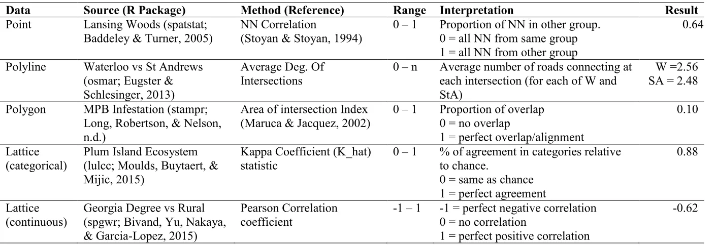
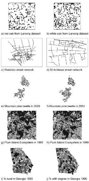
To demonstrate the challenges associated with SPC we have hand-picked a set of five examples 295
(see Table 1 and Figure 3). For each example, we have chosen a representative and current 296
technique for quantitative SPC associated with each data type. In all cases we have selected a 297
single global statistic for comparison. Through the use of basic comparison statistics as a 298
starting point, we highlight some the challenges associated with SPC analysis. 299
< Table 1 Here> 300
<Figure 3 here> 301
4.2. Highlight problems in spatial pattern comparisons 302
Problem 1: Pattern vs Process 303
Perhaps the biggest challenge emerging from the ‘big data’ revolution is that of 304
connecting the analysis of patterns in the data with the underlying processes that we are 305
interested in studying (Miller & Goodchild, 2015). As an example, consider the comparison of 306
the red oak and white oak patterns. The results suggest there is evidence of a relationship 307
between the spatial patterns of the two species, but we do not have any theory to support this 308
at the process level. Perhaps there is inter-species attraction due to seed dispersal, shading 309
11 that this is really of question of spatial interaction at the process level, which manifests in 311
spatial similarity at the pattern level. It is unclear how likely this similarity is under independent 312
spatial processes governing the distribution of red and white oaks. Static spatial patterns are 313
inherently limited in their ability to describe dynamic processes. More data does not necessarily 314
improve this limitation and may in fact add additional noise. 315
Problem 2: Topological Complexity 316
Comparison of topological characteristics of spatial data is typically reduced to 317
comparison of connectivity matrices or graphs. In the example comparing node degree for 318
OSM street networks for Waterloo, Canada and St. Andrews, Scotland. Spatial non-stationarity 319
in road network density in Waterloo was present, whereby node degree of the dense parts of 320
the network in the downtown area more difficult to observe in contrast with the less dense parts 321
of the network in rural outlying areas, which tended to have four-node intersections. The 322
similarity in node degree in the two networks was masked partially by the dis-similarity in 323
network densities. While computing the node-degree values is straightforward, the results here 324
highlight the difficulty in isolating one component of pattern to compare. Typically, the overall 325
comparison of pattern similarity for the HVS is a composite of several dimensions of spatial 326
pattern. Developing metrics or aggregate indicators of similarity of spatial patterns therefore 327
hinges on identifying the key dimensions of pattern for a specific comparison task. Comparing 328
topological properties may be an example where ‘spatial intuition’ and computed values are 329
misaligned, as slight spatial changes can have large impacts on topology (e.g, undershoots in 330
routing problems). 331
Topology is also confounded by spatial representation decisions in maps when 332
visualizing comparisons. The visual assessment of pattern similarity between the mountain 333
pine beetle polygons is certainly impacted by a number of classical cartographic pitfalls, such 334
as a failure to include a reference basemap, map graticule, grid lines, or even a scale bar. 335
However, a much more challenging problem arises when comparing objects that exhibit such 336
a highly complex topology (such as the infestation polygons with irregularly shaped borders, 337
holes, and multiple polygon parts). Had these two infestation polygons exhibited regularly 338
shaped boundaries the comparison process would be easier (both visually, but also 339
computationally). But complex topological shapes, including less binary gradients and 340
boundaries, are the norm in environmental applications (Gustafson, 1998), and are salient in 341
many anthropogenic examples (Batty & Xie, 1994). Thus, characterizing the similarities 342
between complex shapes and patterns in a single (or multiple) index remains an ongoing 343
12 Problem 3: Composition vs Configuration
345
The description of spatial patterns can be decomposed into two unique but 346
interdependent components: composition and configuration (Boots, 1982, 2003). To 347
generalize, composition refers strictly to the aspatial properties of the elements of a spatial 348
pattern (e.g., the type, number, and statistical properties of what is being mapped), while 349
configuration refers to the strictly spatial arrangement of these elements (i.e., the where). 350
Consider the Plum Island Ecosystem maps in Figure 2 (g-h). The most basic description of 351
configuration refers to homogeneous (no variation exists) vs. heterogeneous (i.e., the observed 352
pattern varies across space) spatial patterns. In practice, assessing configuration involves 353
quantifying the level and nature of heterogeneity in mapped data and a wide set of terminology 354
and techniques are available. These terms are typically both data and application specific; and 355
can be used differently depending on the context of the analysis. 356
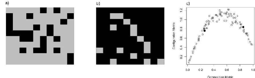
Dependency between composition and configuration of spatial patterns is demonstrated 357
in Figure 4. Previous research has demonstrated that the potential for different spatial 358
configurations to arise is largely dependent on the composition of elements in the map (Remmel 359
& Csillag, 2003; X. Wang & Cumming, 2011). Thus, quantifying SPC is complex due to the 360
potential for changes in configuration to arise solely due to changes in composition (i.e., Figure 361
4), confounding inferences into SPC (Long et al., 2010; Remmel & Csillag, 2003; X. Wang & 362
Cumming, 2011). Indices for SPC must be able to simultaneously consider and disentangle the 363
level of compositional and configurational change to be effective. 364
<Figure 4 here> 365
Problem 4: Spatially Global Indices 366
To date, most approaches for SPC are spatially global, producing a single statistic for 367
the entire study area (indeed all five of the indices we employed fall into this category). With 368
large-area and ‘big’ sources of spatial data, this can be misleading as global statistics fail to 369
adequately capture spatial non-stationarities in observed patterns. However, spatially local 370
analysis of big data also poses challenges since outputs require some interpretation, a non-371
trivial task with increasingly large datasets. With spatial-temporal local models, more 372
sophisticated geovisual analytics may be required to understand the complex output stemming 373
from local analysis of large mapped datasets (Foley & Demšar, 2012). But relying on visual 374
interpretations can be challenging given the characteristics of many modern large datasets (i.e., 375
coverage over broad-scales, with fine spatial resolution). Visualization as a tool for SPC (see 376
13 resolution that is beyond our perceptual limits. Geographic knowledge discovery (Miller & 378
Han, 2009) approaches may be suitable for performing SPC in large geographic databases. 379
A further challenge commonly encountered is that a single output statistic may not be 380
sufficient for performing SPC with complex spatial patterns. For example, the negative 381
correlation identified in the Georgia data may not be consistent across the entire state, and a 382
spatially sensitive correlation measure (e.g., see p. 172 in Fotheringham et al., 2002) would 383
shed further insight into the spatial variation in correlation. With increasingly large datasets 384
(big data), moving the analysis scale from the global to the spatially local scale is necessary to 385
capture how spatial pattern comparisons vary across space. 386
4. Moving the Spatial Pattern Comparison Research Agenda Forward 387
4.1 Comparing maps as spatial processes 388
Csillag and Boots (2005) advocate a process-based framework for comparing spatial 389
patterns and identify two underlying questions that we, as geographers, should be seeking to 390
answer in all SPC related-tasks: 1) Could the observed differences in spatial patterns have 391
arisen purely by chance? and 2) Could the observed spatial patterns have been generated by the 392
same process?. Pearl (2009) makes the case for a clear discrimination between associative and 393
causative statistical analysis where associative analysis considers any relationship that can be 394
defined by joint distribution of two variables and a causative relationship is one that cannot be 395
defined by the joint distribution alone. With respect to SPC nearly all methods would fall into 396
the former category, whilst Csillag and Boots (2005) make the emphatic case for models that 397
fit squarely into the latter. One of the potential areas where new models are providing avenues 398
for new insight along this causative line of thinking is through the development of complex 399
simulations which can be used to test spatially explicit hypotheses (O’Sullivan & Perry, 2013). 400
Spatial analysis theory considers a map as a single realization of a stochastic spatial 401
process, and thus inference regarding two static maps, if treated independently, yields a sample 402
size of two. Spatial inferences pertain to the underlying process, though the particulars of what 403
a mapped pattern represents have been debated (e.g., Summerfield, 1983). Cressie (1993) cites 404
two basic contexts for doing spatial modelling; when a spatial process has reached temporal 405
equilibrium and its spatial properties describe causative components of that process, and when 406
short-term causal effects are aggregated over a fixed time period and expressed spatially. 407
Comparing spatial patterns disconnected from their generative (temporal) processes incurs a 408
high risk of finding differences resulting from natural variability. Explicit incorporation of time 409
into an SPC framework may provide a way to both handle big spatial data and still reason about 410
14 tools for continuous spatial evolution, and 2) undertake spatial multi-pattern comparisons; both 412
which imply a more explicit treatment of spatial processes. 413
Simulations provide an attractive framework for SPC as they allow experimentation 414
with model parameters, incorporation of nonlinear dynamics and feedbacks, and flexibility in 415
the types of model output (e.g., maps) that are generated. Two dominant approaches to 416
simulating spatial patterns and processes are widely used; individual-based models (IBMs), 417
and spatial-covariance models (SVMs). IBMs provide complete flexibility to specify all 418
important dynamics of the geographical system under investigation, which can then be used to 419
draw patterns from the model. Generating reference distributions for SPC metrics can be part 420
of model sensitivity testing. For example, evaluating the model’s sensitivity to parameter 421
uncertainty from the perspective of spatial pattern is an interesting application area for SPC ., 422
Emergent spatial patterns play a central role in developing, parameterizing, and extracting 423
knowledge from IBMs (Grimm et al., 2005), and exemplar spatial patterns for specific 424
processes can be used to find model parameter values through inverse fitting procedures that 425
depend on a pattern comparison metric (Burnham & Anderson, 2002; Wiegand, Revilla, & 426
Knauer, 2004). Such an approach has been recently tested in a more formal framework that 427
provides model selection of parameter values and structure by ‘approximate Bayes’ methods 428
(van der Vaart, Beaumont, Johnston, & Sibly, 2015). The extension of these new approaches 429
for constructing, fitting, and assessing IBMs to incorporate explicitly spatial metrics is an 430
exciting research opportunity for SPC. 431
SVMs instead require specification of the form of spatial pattern that results from the 432
model (or process that generates it), which might more accurately reflect observed data, but 433
tend to have less mechanistic meaning. Remmel et al. (2002) used a conditional autoregressive 434
(CAR) model to simulate three types of landscapes and to compare landscape pattern indices 435
under each landscape-type scenario. The resulting distributions provide reference for 436
interpreting differences between two LPI values when performing landscape. Long et al. (2012) 437
used simulations from a space-time model that incorporated a similar spatial covariance 438
structure (CAR prior) to model the probability of spread of a binary infection process on a 439
lattice. These types of spatial simulations are now widely employed in model testing, 440
comparison, and evaluation where simulated data is used to compare spatial parameter 441
estimates from different model specifications to a known underlying spatial process (e.g., 442
Fotheringham & Oshan, 2016). Currently, visual comparisons and aspatial metrics are the de 443
15 metrics are equally important in the SVM approach, and could perhaps serve as a point of 445
reference for comparing inferences obtained from different modelling frameworks . 446
4.2 Spatially local analysis 447
There is a clear need for robust spatially sensitive metrics, which seems like a surprising 448
thing to be championing given widely available tools for local spatial analysis. However, these 449
tools are largely appropriate only with spatial lattices (regular and irregular) and have failed to 450
be adopted more broadly. In a growing number of applications and decision-making contexts, 451
rigorous definitions of pattern similarity need to be adopted (e.g., Churchill et al., 2013; Sakieh, 452
Amiri, Danekar, Feghhi, & Dezhkam, 2015). When numeric or categorical data are obtained 453
over comparable spatial units and the SPC task pertains to how that data are spatially 454
configured across those units, measures of spatial pattern such as Moran’s I, Geary’s C, or local 455
variants can be employed. Waller (2014) provides a convincing argument for the need for 456
explicitly spatial statistical thinking in approaching analysis of geographical data, citing 457
common research motivations such as assessing fit of spatial models or spatial assessment of 458
statistical performance. Methods for SPC reviewed here can directly contribute to development 459
of a spatial statistical approach to science by providing tools for the robust comparison of 460
spatial patterns. 461
Yet the methods needed to answer comparative questions are often lacking. To 462
demonstrate this, a linear regression performed between ‘% rural’ and ‘% with a college 463
degree’ from the Georgia dataset, and the residuals were retained and shuffled across the 464
counties randomly (Figure 5). Two very different spatial patterns emerge which have identical 465
error statistics (MAE 0, RMSE 4.46). A reasonable question might be to ask whether the 466
differences are due to chance or the result of different underlying spatial processes, or rather, 467
what are the chances of obtaining I= -0.169 and I = 0.274 from this configuration of spatial 468
units and values, if the underlying processes are the same. Given the exact distribution of 469
Moran’s I (Tiefelsdorf & Boots, 1995) we can compute probabilities of observed patterns based 470
on a null hypothesis of no spatial structure, but cannot use these results to compare two patterns 471
directly. Tiefelsdorf (1998) gives a conditional expectation of Moran’s which allows 472
comparison of competing spatial process hypotheses as expressed through the spatial weights 473
matrix. Clifford et al. (1989) provide a t-test for comparing spatial structure in the context of a 474
correlation coefficient, yet do not give us a tool to understand if the spatial process giving rise 475
to the two patterns is the same or not. 476
<Figure 5 here> 477
16 Spatial scale is often determined either arbitrarily or by a fixed set of intervals – both 479
in terms of grain and extent. This is critical for SPC because scale is intimately tied to the 480
definition of and observation of spatial patterns (Levin 1992; Dale 2000). The infinite number 481
of scales available for both making observations (i.e. grain) as well as observing patterns (i.e., 482
extent), and the inter-relatedness of these constructs, makes comparison tasks challenging. Not 483
all scales are created equal for a given problem, and a set of characteristic scales are optimal 484
for analysis (Wiens, 1989). Big data provides opportunities for linking spatial processes across 485
scales, especially if data evolve over time. Previously, issues of scale in geographical analysis 486
tended to focus on the modifiable areal unit problem, whereby ‘scale effects’ are assessed by 487
varying aggregation units (e.g., Jelinski, Wu, & Wu, 1996). For SPC problems, variances due 488
to scale may be a critical aspect of pattern-observation and thus comparison. Sémécurbe et al. 489
(2016) provide an example of using multifractal analysis that quantifies MAUP to better 490
understand spatial heterogeneities in population density in France, developing a typology of 491
settlement patterns. 492
Yan and Li (2015) stress the need for both mathematical and psychological 493
justifications in the definition of spatial similarity measures (i.e., linking similarity to the HVS). 494
For the case of automated map generalization, a hierarchical scheme of maps, layers, groups, 495
and objects (i.e., points, lines, areas) is presented which define the fundamental units for which 496
spatial similarity relations are sought. The relations for comparing spatial objects at different 497
scales are distinct from the comparison of patterns. In the Yan and Li system, object properties 498
(size, shape, area etc.) and object group properties (topology, distance, correction etc.) may be 499
a way to integrate dimensions of similarity at the pattern or regional scale. 500
4.4 Guidance for performing SPC 501
We provide six simple guidelines for researchers wishing to compare spatial patterns in their 502
own applications. 503
1. Visual comparisons are useful – comparing two maps visually is a crucial first step in 504
the exploratory spatial data analysis process. 505
2. Quantitative measures are necessary – the subjectivity of the visual comparison process 506
means that any visual comparison should be further explored using a quantitative 507
comparison metric. 508
3. Local SPC measures are preferred – global SPC measures are subject to all the issues 509
17 4. Quantifying dissimilarity is better – indices that focus on characterizing differences in 511
patterns, over similarities in pattern are more likely to provide meaningful inferences 512
(Pontius Jr & Millones, 2011). 513
5. Consider multiple elements of spatial pattern – spatial patterns have a variety of 514
characteristic components. Comparison measures capable of disentangling different 515
elements of spatial pattern within the SPC context are more informative than summary 516
measures. 517
6. Don't forget processes – understanding the linkages between processes and patterns is 518
the most challenging part of spatial analysis. Quantified pattern (dis)similarities may 519
be related to unknown confounding processes. 520
521
5 Conclusions 522
SPC is a complex task, which is difficult to automate, has a mixture of computational 523
and psychological components, and is increasingly required as geography and other fields 524
exploit bigger and more varied spatial datasets. Here we have reviewed the literature on SPC 525
that comes from a wide array of disciplines where applied problems have developed specific 526
comparison methods, lacking any coherent conceptual or theoretical framework. Our review 527
has focused on comparing spatial patterns of similar spatial representations (e.g., point-point, 528
lattice-lattice), there are however significant prospects for developing new methods for ‘off-529
diagonal’ comparisons (e.g., point-polygon, line-lattice etc.). Many of the classical problems 530
of geography such as pattern vs process, scale, MAUP, and topology become exacerbated in 531
SPC. The spatial patterns we observe in maps are determined partially by spatial representation, 532
aspatial characteristics, data collection components, the truly spatial component, and some 533
element of randomness. More research into how these various components interact to create 534
spatial distributions we observe, through simulation and empirical data catalogs, would bolster 535
our ability to develop spatial modeling tools that support SPC. 536
537
1 References
1
Andersen, M. (1992). Spatial analysis of two-species interactions. Oecologia, 91, 134–140. 2
Austin, S. B., Melly, S. J., Sanchez, B. N., Patel, A., Buka, S., & Gortmaker, S. L. (2005). 3
Clustering of fast-food restaurants around schools: A novel application of spatial 4
statistics to the study of food environments. American Journal of Public Health, 95, 5
1575–1581. 6
Baddeley, A., & Turner, R. (2005). Spatstat: an R package for analyzing spatial point 7
patterns. Journal of Statistical Software, 12, 1–42. 8
Batty, M., & Xie, Y. (1994). Modelling inside GIS: Part 1. Models structures, exploratory 9
spatial data analysis and aggregation. International Journal of Geographical 10
Information Systems, 8, 291–307. 11
Bell, M. L., & Grunwald, G. K. (2004). Mixed models for the analysis of replicated spatial 12
point patterns. Biostatistics, 5, 633–648. 13
Bennett, N. D., Croke, B. F. W., Guariso, G., Guillaume, J. H. a, Hamilton, S. H., Jakeman, 14
A. J., … Andreassian, V. (2013). Characterising performance of environmental models. 15
Environmental Modelling & Software, 40, 1–20. 16
Bivand, R. S., Yu, D., Nakaya, T., & Garcia-Lopez, M. A. (2015). Package “spgwr.” 17
Boots, B. (1982). Comments on the use of eigenfunctions to measure structural properties of 18
geographic networks. Environment and Planning A, 14, 1063–1072. 19
Boots, B. (2003). Developing local measure of spatial ssociation for categorical data. Journal 20
of Geographical Systems, 5, 139–160. 21
Boots, B., & Csillag, F. (2006). Categorical maps, comparisons, and confidence. Journal of 22
Geographical Systems, 8, 109–118. 23
Boots, B., & Okabe, A. (2007). Local statistical spatial analysis: Inventory and prospect. 24
International Journal of Geographical Information Science, 21, 355–375. 25
Bunn, A. G., Urban, D. L., & Keitt, T. H. (2000). Landscape connectivity: A conservation 26
application of graph theory. Journal of Environmental Management, 59, 265–278. 27
Burguet, J., & Andrey, P. (2014). Statistical comparison of spatial point patterns in biological 28
2 Burnham, K. P., & Anderson, D. R. (2002). Model selection and multi-model inference: a 30
practical information-theoretic approach. Springer. 31
Churchill, D. J., Larson, A. J., Dahlgreen, M. C., Franklin, J. F., Hessburg, P. F., & Lutz, J. 32
A. (2013). Restoring forest resilience: From reference spatial patterns to silvicultural 33
prescriptions and monitoring. Forest Ecology and Management, 291, 442–457. 34
Cliff, A. (1970). Computing the spatial correspondence between geographical patterns. 35
Transaction of the Institute of British Geographers, 50, 143–154. 36
Cliff, A., & Ord, J. K. (1973). Spatial Autocorrelation. London: Pion Limited. 37
Clifford, P., Richardson, S., & Hemon, D. (1989). Assessing the significance of the 38
correlation between two spatial processes. Biometrics, 45, 123–134. 39
Cressie, N. (1993). Statistics for Spatial Data. New York: John Wiley & Sons Inc. 40
Csillag, F., & Boots, B. (2005). A framework for statistical inferential decisions in spatial 41
pattern analysis. The Canadian Geographer, 49, 172–179. 42
Csillag, F., & Boots, B. (2005). Toward comparing maps as spatial processes. In 43
Developments in Spatial Data Handling (pp. 641–652). 44
Cushman, S. A., McGarigal, K., & Neel, M. C. (2008). Parsimony in landscape metrics: 45
Strength, universality, and consistency. Ecological Indicators, 8, 691–703. 46
Dale, M. (2000). Spatial Pattern Analysis in Plant Ecology. Cambridge: Cambridge 47
University Press. 48
Diggle, P. J. (2003). Statistical Analysis of Spatial Point Patterns (2nd ed.). New York, NY: 49
Arnold. 50
Eugster, M. J. A., & Schlesinger, T. (2013). osmar: OpenStreetMap and R. The R Journal, 5, 51
53–63. 52
Foley, P., & Demšar, U. (2012). Using geovisual analytics to compare the performance of 53
geographically weighted discriminant analysis versus its global counterpart, linear 54
discriminant analysis. International Journal of Geographical Information Science, 27, 55
633–661. 56
Fotheringham, A. S., & Brunsdon, C. (1999). Local forms of spatial analysis. Geographical 57
3 Fotheringham, A. S., Brunsdon, C., & Charlton, M. (2002). Geographically Weighted
59
Regression: The Analysis of Spatially Varying Relationships. Chichester: Wiley. 60
Fotheringham, A. S., & Oshan, T. M. (2016). Geographically weighted regression and 61
multicollinearity: dispelling the myth. Journal of Geographical Systems, 18, 303–329. 62
Goodchild, M. F., & Hunter, G. J. (1997). A simple positional accuracy measure for linear 63
features. International Journal of Geographical Information Science, 11, 299–306. 64
Grimm, V., Revilla, E., Berger, U., Jeltsch, F., Mooij, W. M., Railsback, S. F., … DeAngelis, 65
D. L. (2005). Pattern-oriented modeling of agent-based complex systems: lessons from 66
ecology. Science, 310, 987–991. 67
Gustafson, E. (1998). Quantifying landscape spatial pattern: what is the state of the art? 68
Ecosystems, 1, 143–156. 69
Hagen-Zanker, A. (2009). An improved Fuzzy Kappa statistic that accounts for spatial 70
autocorrelation. International Journal of Geographical Information Science, 23, 61–73. 71
Hagen-Zanker, A., & Martens, P. (2008). Map comparison methods for comprehensive 72
assessment of geosimulation models. Computational Science and Its Applications– 73
ICCSA 2008, 194–209. 74
Hägerstrand, T. (1967). On Monte Carlo simulation of diffusion. Quantitative Geography, 75
Part, 1, 1–32. 76
Haining, R. (1991). Bivariate correlation with spatial data. Geographical Analysis, 23, 210– 77
227. 78
Hengl, T., Heuvelink, G. B. M., & Stein, A. (2004). A generic framework for spatial 79
prediction of soil variables based on regression-kriging. Geoderma, 120, 75–93. 80
Hubert, L. J., Golledge, R. G., Costanzo, C. M., Gale, N., Costanzo, M., & Gale, N. (1985). 81
Measuring association between spatially defined variables: An alternative procedure. 82
Geographical Analysis, 17, 37–46. 83
IPCC. (2014). Climate Change 2014 Synthesis Report. In I. Core Writing Team, R. Pachauri, 84
& L. Meyer (Eds.), Contribution of Working Groups I, II and III to the Fifth Assessment 85
Report of the Intergovernmental Panel on Climate Change (p. 151). Geneva: IPCC. 86
Jacobs, D. E., Goldman, D. B., & Shechtman, E. (2010). Cosaliency: where people look 87
4 interface software and technology, 219–228.
89
Jasiewicz, J., Netzel, P., & Stepinski, T. F. (2014). Landscape similarity, retrieval, and 90
machine mapping of physiographic units. Geomorphology, 221, 104–112. 91
Jelinski, D. E., Wu, & Wu, J. (1996). The modifiable areal unit problem and implications for 92
landscape ecology. Landscape Ecology, 11, 129–140. 93
Jones, E. L., Rendell, L., Pirotta, E., & Long, J. A. (2016). Novel application of a quantitative 94
spatial comparison tool to species distribution data. Ecological Indicators, 70, 67–76. 95
Kranstauber, B., Smolla, M., & Safi, K. (2016). Similarity in spatial utilization distributions 96
measured by the earth mover’s distance. Methods in Ecology and Evolution. 97
doi:10.1111/2041-210X.12649 98
Lee, S.-I. (2001). Developing a bivariate spatial association measure: An integration of 99
Pearson’s r and Moran’s I. Journal of Geographical Systems, 3, 369–385. 100
Levin, S. (1992). The problem of pattern and scale in ecology. Ecology, 73, 1943–1967. 101
Li, S., Dragicevic, S., Castro, F. A., Sester, M., Winter, S., Coltekin, A., … Cheng, T. (2016). 102
Geospatial big data handling theory and methods: A review and research challenges. 103
ISPRS Journal of Photogrammetry and Remote Sensing, 115, 119–133. 104
Lloyd, R., & Steinke, T. (1977). Visual and Statistical Comparison of Choropleth Maps. 105
Annals of the Association of American Geographers, 67, 429–436. 106
Lobo, M.-J., Pietriga, E., & Appert, C. (2015). An Evaluation of Interactive Map Comparison 107
Techniques. In CHI’15 Proceedings of the 33rd Annual ACM Conference on Human 108
Factors in Computing Systems (pp. 3573–3582). Seoul, South Korea: ACM. 109
Long, J. A., Nelson, T. A., & Wulder, M. A. (2010). Characterizing forest fragmentation: 110
Distinguishing change in composition from configuration. Applied Geography, 30, 426– 111
435. 112
Long, J. A., Robertson, C., Nathoo, F. S., & Nelson, T. A. (2012). A Bayesian space-time 113
model for discrete spread processes on a lattice. Spatial and Spatio-Temporal 114
Epidemiology, 3, 151–62. 115
Long, J. A., Robertson, C., & Nelson, T. A. (n.d.). stampr: An R package for spatial-temporal 116
analysis of moving polygons. Journal of Statistical Software, In Review, 18p. 117
5 New York: The Guilford Press.
119
Marr, D. (1985). Vision: The philosophy an the approach. In A. M. Aitkenhead & J. M. Slack 120
(Eds.), Issues in Cognitive Modeling (pp. 103–126). London: Erlbaum. 121
Maruca, S. L., & Jacquez, G. M. (2002). Area-based tests for association between spatial 122
patterns. Journal of Geographical Systems, 4, 69–83. 123
Miller, H. J., & Goodchild, M. F. (2015). Data-driven geography. GeoJournal, 80, 449–461. 124
Miller, H. J., & Han, J. (2009). Geographic data mining and knowledge discovery An 125
Overview. In Geographic data mining and knowledge discovery (pp. 1–26). 126
Miller, H. J., & Wentz, E. a. (2003). Representation and Spatial Analysis in Geographic 127
Information Systems. Annals of the Association of American Geographers, 93, 574–594. 128
Mladenoff, D. J., White, M. A., Pastor, J., & Crow, T. R. (1993). Comparing spatial pattern 129
in unaltered old-growth and disturbed forest landscapes. Ecological Applications, 3, 130
294–306. 131
Moulds, S., Buytaert, W., & Mijic, A. (2015). An open and extensible framework for 132
spatially explicit land use change modelling: the lulcc R package. Geosci. Model Dev., 133
8, 3215–3229. 134
Myers, G. (2012). Why bioimage informatics matters. Nature Methods, 9, 659–660. 135
O’Sullivan, D., & Perry, G. L. W. (2013). Spatial Simulation: Exploring Pattern and 136
Process. John Wiley & sons. 137
O’Sullivan, D., & Unwin, D. (2010). Geographic Information Analysis (2nd ed.). Hoboken, 138
NJ: John Wiley & Sons. 139
Openshaw, S., & Abrahart, R. J. (1996). Geocomputation. In R. J. Abrahart (Ed.), 1st 140
International Conference on GeoComputation (pp. 665–666). University of Leeds, UK. 141
Ord, K., & Getis, A. (2001). Testing for local spatial autocorrelation in the presence of global 142
autocorrelation. Journal of Regional Science, 41, 411–432. 143
Pearl, J. (2009). Causality: Models, Reasoning and Inference (2nd ed.). Cambridge: 144
Cambridge University Press. 145
Plouffe, C. C. F., Robertson, C., & Chandrapala, L. (2015). Comparing interpolation 146
6 data sources: A case study of Sri Lanka. Environmental Modelling & Software, 67, 57– 148
71. 149
Pontius Jr, R. G., & Millones, M. (2011). Death to Kappa: birth of quantity disagreement and 150
allocation disagreement for accuracy assessment. International Journal of Remote 151
Sensing, 32, 4407–4429. 152
Remmel, T., & Csillag, F. (2003). When are two landscape pattern indexes significantly 153
different. Journal of Geographical Systems, 5, 331–351. 154
Remmel, T., Csillag, F., Mitchell, S. W., & Boots, B. (2002). Empirical distributions of 155
landscape pattern indices as functions of classified image composition and spatial 156
structure. Ottawa, Ontario, Canada. 157
Roberts, S., & Robertson, C. (2016). Geographic Information Systems and Science: A 158
Concise Handbook of Spatial Data Handling, Representation, and Computation. Don 159
Mills, Ontario: Oxford University Press. 160
Robertson, C., Long, J. A., Nathoo, F. S., Nelson, T. A., & Plouffe, C. C. F. C. F. (2014). 161
Assessing quality of spatial models using the structural similarity index and posterior 162
predictive checks. Geographical Analysis, 46, 53–74. 163
Robertson, C., Nelson, T. A., Boots, B., & Wulder, M. A. (2007). STAMP: spatial–temporal 164
analysis of moving polygons. Journal of Geographical Systems, 9, 207–227. 165
Robinson, A. H. H., & Bryson, R. A. (1957). A Method for Describing Quantitivatively the 166
Correspondence of Geographic Distributions. Annals of the Association of American 167
Geographers, 47, 379–391. 168
Rubner, Y., Tomasi, C., & Guibas, L. J. (2000). The earth mover’s distance as a metric for 169
image retrieval. International Journal of Computer Vision, 40, 99–121. 170
Sadahiro, Y., & Umemura, M. (2001). A computational approach for the analysis of changes 171
in polygon distributions. Journal of Geographical Systems, 3, 137–154. 172
Sakieh, Y., Amiri, B. J., Danekar, A., Feghhi, J., & Dezhkam, S. (2015). Scenario-based 173
evaluation of urban development sustainability: an integrative modeling approach to 174
compromise between urbanization suitability index and landscape pattern. Environment, 175
Development and Sustainability, 17, 1343–1365. 176
7 12th International Conference on Pattern Recognition, 1.
178
doi:10.1109/ICPR.1994.576363 179
Sémécurbe, F., Tannier, C., & Roux, S. G. (2016). Spatial distribution of human population 180
in France: Exploring the modifiable areal unit problem using multifractal analysis. 181
Geographical Analysis, 48, 292–313. 182
Shao, Z., Zhou, W., Zhang, L., & Hou, J. (2014). Improved color texture descriptors for 183
remote sensing image retrieval. Journal of Applied Remote Sensing, 8, 83584. 184
Shaw, S.-L., Tsou, M.-H., & Ye, X. (2016). Editorial: human dynamics in the mobile and big 185
data era. International Journal of Geographical Information Science, 30, 1687–1693. 186
Sokal, R. R., & Wartenberg, D. E. (1983). A test of spatial autocorrelation analysis using an 187
isolation-by-distance model. Genetics, 105, 219–237. 188
Spielman, S. E., & Thill, J. C. (2008). Social area analysis, data mining, and GIS. Computers, 189
Environment and Urban Systems, 32, 110–122. 190
Steinke, T., & Lloyd, R. (1983). Judging the similarity of choropleth map images. 191
Cartographica, 20, 35–24. 192
Stoyan, D., & Stoyan, H. (1994). Fractals, Random Shapes and Point Fields: Methods of 193
Geometrical Statistics. (J. W. & Sons, Ed.). Chichester, New York. 194
Summerfield, M. (1983). Populations, samples, and statistical inference in geography. The 195
Professional Geographer, 35, 143–149. 196
Syrjala, S. E. (1996). A Statistical Test for a Difference between the Spatial Distributions of 197
Two Populations. Ecology, 77, 75–80. 198
Tiefelsdorf, M. (1998). Some practical applications of Moran’s I’s exact conditional 199
distribution. Papers in Regional Science, 77, 101–129. 200
Tiefelsdorf, M., & Boots, B. (1995). The exact distribution of Moran’s I. Environment and 201
Planning A, 27, 985–999. 202
Tobler, W. (1965). Computation of the correspondence of geographical patterns. Papers of 203
the Regional Science Association, 15, 131–139. 204
Turner, M. G. (1989). Landscape ecology: The effect of pattern on process. Annual Review of 205
8 Urban, D. L., & Keitt, T. (2001). Landscape connectivity: A graph-theoretic perspective. 207
Ecology, 82, 1205–1218. 208
Urban, D. L., Minor, E. S., Treml, E. A., & Schick, R. S. (2009). Graph models of habitat 209
mosaics. Ecology Letters, 12, 260–273. 210
van der Vaart, E., Beaumont, M. A., Johnston, A. S. A., & Sibly, R. M. (2015). Calibration 211
and evaluation of individual-based models using approximate Bayesian computation. 212
Ecological Modelling, 312, 182–190. 213
Visser, H., & de Nijs, T. (2006). The Map Comparison Kit. Environmental Modelling & 214
Software, 21, 346–358. 215
Waller, L. A. (2014). Putting spatial statistics (back) on the map. Spatial Statistics, 9, 4–19. 216
Wang, X., & Cumming, S. G. (2011). Measuring landscape configuration with normalized 217
metrics. Landscape Ecology, 26, 723–736. 218
Wang, Z., Bovik, A. C., Sheikh, H. R., & Simoncelli, E. P. (2004). Image Quality 219
Assessment : From Error Visibility to Structural Similarity. IEEE Transactions on Image 220
Processing, 13, 600–612. 221
Wheeler, D. C. (2010). Visualizing and Diagnosing Coefficients from Geographically 222
Weighted Regression Models. In B. Jiang & X. Yao (Eds.), Geospatial Analysis and 223
Modelling of Urban Structure and Dynamics (Vol. 99, pp. 415–436). Berlin: Springer 224
Science and Business Media. 225
Wiegand, T., Revilla, E., & Knauer, F. (2004). Dealing with uncertainty in spatially explicit 226
population models. Biodiversity & Conservation, 13, 53–78. 227
Wiens. (1989). Spatial scaling in ecology. Functional Ecology, 3, 385–397. 228
Wong, D. (2001). Location specific cumulative distribution function (LSCDF): An 229
alternative to spatial correlation analysis. Geographical Analysis, 33, 76–93. 230
Wulder, M. A., Boots, B., Seemann, D., & White, J. C. (2004). Map comparison using spatial 231
autocorrelation : an example using AVHRR derived land cover of Canada. The 232
Canadian Geographer, 30, 573–592. 233
Yan, H., & Li, J. (2015). Spatial Similarity Relations in Multi-scale Map Spaces. Heidelberg: 234
Springer. doi:10.1007/978-3-319-09743-5 235
9 IEEE Transactions on Geoscience and Remote Sensing, 51, 818–832.
1 Box 1: Glossary of terms.
Spatial Pattern Comparison - a numerical assessment of the (dis)similarity between two (or more) mapped datasets.
Spatial Pattern - scale-dependent predictability of the physical arrangement of observations Spatial Process – model that produces spatial patterns with a known probabilistic function Global Statistic – summary statistic that quantifies a property of spatial distribution with a single value
Local Statistic - summary statistic that quantifies a property of a spatial distribution at each location and sums to a global statistic
1 Table 1: Example datasets and methods for exploring issues in spatial pattern comparison analysis.
Data Source (R Package) Method (Reference) Range Interpretation Result
Point Lansing Woods (spatstat; Baddeley & Turner, 2005)
NN Correlation
(Stoyan & Stoyan, 1994)
0 – 1 Proportion of NN in other group. 0 = all NN from same group 1 = all NN from other group
0.64
Polyline Waterloo vs St Andrews (osmar; Eugster & Schlesinger, 2013)
Average Deg. Of Intersections
0 – n Average number of roads connecting at each intersection (for each of W and StA)
W =2.56 SA = 2.48
Polygon MPB Infestation (stampr; Long, Robertson, & Nelson, n.d.)
Area of intersection Index (Maruca & Jacquez, 2002)
0 – 1 Proportion of overlap 0 = no overlap
1 = perfect overlap/alignment
0.10
Lattice (categorical)
Plum Island Ecosystem (lulcc; Moulds, Buytaert, & Mijic, 2015)
Kappa Coefficient (K_hat) statistic
0 – 1 % of agreement in categories relative to chance.
0 = same as chance 1 = perfect agreement
0.88
Lattice (continuous)
Georgia Degree vs Rural (spgwr; Bivand, Yu, Nakaya, & Garcia-Lopez, 2015)
Pearson Correlation coefficient
-1 – 1 -1 = perfect negative correlation 0 = no correlation
1 = perfect positive correlation
1 Figures