Coupled complex networks : structure, adaptation and processes

ADAPTATION, AND PROCESS

S

aray Shai

A Thesis Submitted for the Degree of PhD at the

University of St Andrews

2014

Full metadata for this item is available in Research@StAndrews:FullText

at:

http://research-repository.st-andrews.ac.uk/

Please use this identifier to cite or link to this item:

http://hdl.handle.net/10023/6596

adaptation, and processes

Saray Shai

This thesis is submitted in partial fulfilment for the degree of

Doctor of Philosophy

at the University of St Andrews

In the last 15 years, network science has established itself as a leading scientific tool for the study of complex systems, describing how components in a system interact with one another. Understanding the structure and dynamics of these networks of interactions is the key to understanding the global behaviour of the systems they represent, with a wide range of applications to fundamental societal problems; from designing stable and resilient infrastructures which are critical to our sustainability, to identifying topological patterns in interactome networks that are associated with breast cancer.

Most studies so far have focused on isolated single networks that do not interact with or depend upon other networks, while in reality networks rarely live in isolation and are often just one component in a much larger complex multilevel network. Together with the increased availability of richer, bigger and multi-relational datasets, the analysis of coupled networks has been recently attracting many researchers, and has exposed a multitude of new features and phenomena that were not observed for isolated networks.

In this thesis, we present analytical, numerical and empirical studies of coupled complex networks, aiming to understand the implications of coupling to the functionality and behaviour of complex systems.

First of all, I would like to thank my supervisor Prof. Simon Dobson for showing me how to enjoy research. This thesis would not have been possible without him and without his great advice, support and encouragement he has given me over the last four years.

I am also thankful for the further advice and inspiration I have received from my second supervisors Prof. Ian Gent and Prof. Jane Hillston.

I would like to thank my committee members Prof. Stephen Linton and Prof. David Arrowsmith for a stimulating discussion during my viva, and for their useful suggestions.

I also thank my friends and colleagues in the School of Computer Science, who are always there for me, supporting and inspiring my research, equally happy to have a stimulating discussion or an early afternoon pint.

Some of the work presented in this thesis has been previously published:

I Saray Shai and Simon DobsonEffect of resource constraints on intersimilar

coupled networks. Phys Rev E 86(6): 066120 (2012)

II Saray Shai and Simon DobsonCoupled adaptive complex networks. Phys Rev E 87(4): 042812 (2013)

III Saray Shai, Dror Y. Kenett, Yoed N. Kenett, Miriam Faust, Simon Dobson and Shlomo Havlin Resilience of modular complex networks. Manuscript submitted for publication. arXiv:1404.4748 (2014)

IV Emanuele Strano, Saray Shai, Simon Dobson and Marc BarthélemyEfficiency

and centrality of multiplex spatial networks in large urban areas. Manuscript

Candidate’s Declarations

I, Saray Shai, hereby certify that this thesis, which is approximately 31 113 words in length, has been written by me, that it is the record of work carried out by me and that it has not been submitted in any previous application for a higher degree.

I was admitted as a research student and as a candidate for the degree of Doctor of Philosophy in September 2010; the higher study for which this is a record was carried out in the University of St Andrews between 2010 and 2014.

Date:

Signature of candidate:

Supervisor’s Declaration

I hereby certify that the candidate has fulfilled the conditions of the Resolution and Regulations appropriate for the degree of Doctor of Philosophy in the University of St Andrews and that the candidate is qualified to submit this thesis in application for that degree.

Date:

In submitting this thesis to the University of St Andrews I understand that I am giving permission for it to be made available for use in accordance with the regulations of the University Library for the time being in force, subject to any copyright vested in the work not being affected thereby. I also understand that the title and the abstract will be published, and that a copy of the work may be made and supplied to any bona fide library or research worker, that my thesis will be electronically accessible for personal or research use unless exempt by award of an embargo as requested below, and that the library has the right to migrate my thesis into new electronic forms as required to ensure continued access to the thesis. I have obtained any third-party copyright permissions that may be required in order to allow such access and migration, or have requested the appropriate embargo below.

The following is an agreed request by candidate and supervisor regarding the electronic publication of this thesis:

Access to printed copy and electronic publication of thesis through the University of St Andrews.

Date:

Signature of candidate:

Contents i

List of Figures iii

1 Introduction 1

1.0.1 Contributions of this thesis . . . 3

1.0.2 Structure . . . 4

2 Background 7 2.1 Basic concepts in network theory . . . 7

2.1.1 Degree distribution . . . 8

2.1.2 The small-world effect . . . 10

2.1.3 Clustering . . . 10

2.1.4 Giant component . . . 11

2.2 Network models . . . 12

2.2.1 The Erd˝os-Rényi model . . . 12

2.2.2 Watts-Strogatz small-world networks . . . 13

2.2.3 Barabási-Albert preferential attachment model . . . 13

2.2.4 Configuration model . . . 14

2.3 Dynamics on networks . . . 16

2.3.1 Percolation and network resilience . . . 16

2.3.2 Epidemic spreading . . . 20

2.4 Coupled networks . . . 24

2.4.1 Interdependent networks . . . 25

2.4.2 Interacting, modular, and multiplex networks . . . 28

2.5 Conclusions . . . 31

3 Resilience of modular networks 33 3.1 Introduction . . . 33

3.2 Model of random modular networks . . . 35

3.3 Analytical framework . . . 37

3.3.1 Generating functions for networks of networks . . . 38

3.3.2 Solution for modular ER networks . . . 39

3.3.3 Attack on interconnected nodes . . . 41

3.4 Results . . . 45

3.5 Conclusion . . . 52

4 Epidemic spreading on coupled adaptive networks 55

4.1 Introduction . . . 55

4.2 Model . . . 57

4.3 Formalism . . . 58

4.4 Simulation . . . 64

4.5 Results . . . 65

4.6 Conclusion . . . 70

5 Constrained epidemic spreading on correlated coupled networks 73 5.1 Introduction . . . 73

5.2 Model . . . 76

5.3 Simulation . . . 77

5.4 Results . . . 78

5.5 Conclusion . . . 85

6 Empirical study of coupled transportation networks 87 6.1 Introduction . . . 88

6.2 Data and methods . . . 91

6.2.1 Computing quickest paths . . . 94

6.3 Results . . . 94

6.3.1 Quickest paths . . . 94

6.3.2 Interdependence . . . 96

6.3.3 Centralities . . . 98

6.3.4 Local outreach . . . 101

6.4 Discussion . . . 103

7 Conclusions 107 7.0.1 Contributions . . . 109

7.0.2 Discussion . . . 109

2.1 Schematic illustration of an undirected network . . . 8

2.2 Scale free vs. exponential degree distribution . . . 9

2.3 Construction of the Watts-Strogatz small-world model . . . 13

2.4 Visualisation of random networks generated with different network formation models 15 2.5 Robustness of scale-free and exponential networks to attack and random failure . . 21

2.6 Second order vs. first order percolation transition . . . 26

3.1 Schematic illustration of a modular network . . . 34

3.2 Modular networks generated with different values ofα . . . 37

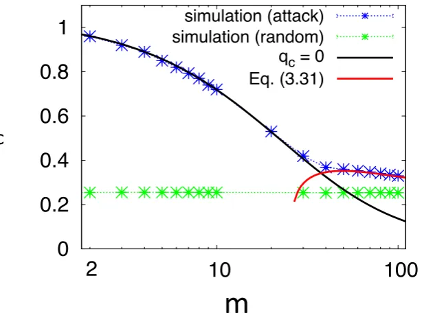
3.3 Percolation threshold as a function of the number of modules . . . 46

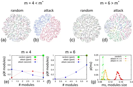
3.4 Visualisation of the network where the giant component contains 10% of the nodes 47 3.5 Size of the largest connected component as a function of the occupation probability 49 3.6 Critical number of modules as a function ofα . . . 49

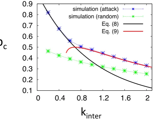
3.7 Percolation threshold as a function of the mean inter-module degree . . . 50

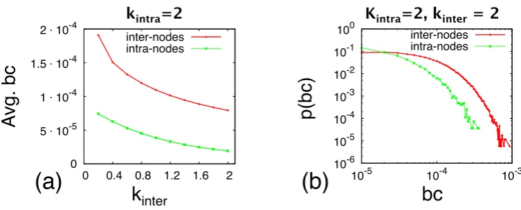
3.8 Betweenness centrality of interconnected vs. intraconnected nodes . . . 51

3.9 Two percolation regimes in scale-free modular networks . . . 52

4.1 Bifurcation diagram of stationary disease prevalences with no rewiring . . . 66

4.2 Bifurcation diagram of stationary disease prevalences with rewiring rateγ=0.04 . . 67

4.3 Localise epidemic breakout only in the coupled nodes . . . 68

4.4 Analytical results without pair approximation . . . 69

5.1 Epidemic transition as a function of the infection rate . . . 78

5.2 Degree distributions of constrained and non-constrained correlated multiplex networks 80 5.3 Degree-degree correlations in correlated multiplex networks . . . 82

5.4 Degree-degree correlations in single BA networks . . . 83

5.5 Epidemic transition as a function of the interaction limit . . . 84

6.1 Spatial and statistical distribution of cells sizes in London . . . 89

6.2 Distinctive features of betweenness centrality in real street networks . . . 90

6.3 The spatial extent of the two datasets of London and New York . . . 92

6.4 Basic quantitative analysis of underground and street networks . . . 93

6.5 Distribution of quickest paths . . . 95

6.6 Interdependence between underground and street networks . . . 96

6.7 Interdependence profile . . . 97

6.8 Effect of coupling on the spatial distribution of betweenness centrality . . . 99

1

C

HAPTER

O

NE

I

NTRODUCTION

Complexity is a young discipline which can help us understand the world around us.

Self-organising emergent complex systems, in which large networks of components with no central

control and simple rules of operation give rise to complex collective behaviour, are ubiquitous

across disciplines [160]. In a cell, the complex network of chemical constituents and reactions

play a key role in sustaining cellular functions [135]; our society is shaped by a network of

repeated local interactions among individuals, which give rise to global regularities such as

spontaneous formation of a common language and culture or the emergence of consensus about a specific issue [62]; even large-scale engineered systems, such as energy distribution

networks [9], transportation networks [26] and the Internet [94], often evolve from the bottom up

in a decentralised manner, growing complex structural patterns resulting from local optimisations

and decision-making at different scales.

Although very different in nature, the systems mentioned above can all be abstracted into

networks (or graphs), by describing which components in a system interact with one another,

thus hiding the complexity of their constituting parts and concentrating on their connectivity patterns instead. The analysis of networks of interactions has proven useful in a wide range

of systems and have recently become the focus of a dedicated research field called “network

science”. But the idea of abstracting complex problems away from their details into the language

of graphs and then use general mathematical tools to manipulate them, is not new. It was

originally invented in 1736 by one of the best-known mathematicians, Leonhard Euler, using

which he solved the famous Königsberg Bridges problem (consisting in finding a round trip

that traversed each of the bridges of the prussian city of Königsberg exactly once), and founded

modern graph theory [44, 93]. Since its birth, graph theory has been established as a branch of

discrete mathematics with stimulating problems such as graph colouring, covering and max-flow problems.

Recent years, however, have witnessed a substantial new movement in network research, with the

focus shifting away from the analysis of networks small enough to be described in full, with all

their nodes, edges and other details written down, to general statements about the properties of

large-scale networks, whose complete details might not be known. It began with the introduction

of random graphs by the Hungarian mathematicians Paul Erd˝os and Alfred Rényi, who studied

the statistical properties of graphs generated by a random process [45, 89, 90]. Erd˝os and Rényi

random graph model has guided our thinking about complex networks for decades since its

introduction and is still widely used in many fields and serve as a benchmark for many modelling and empirical studies. But with the recent availability of large databases of various real networks,

coupled with an increased computational ability to analyse them, the topology of real networks

has been found to largely deviate from a random graph, calling for new tools and measurements to

quantify their underlying organising principles, and leading the emergence of “network science”.

Remarkably, it was discovered that the connectivity patterns of fundamentally different systems,

including the World Wide Web [12] and the Internet [94], scientific coauthorship and citation

networks [170], and neural and metabolic networks [55, 135], display common universal features, such as very large fluctuations in the number of connections – most of their nodes are very

low connected, but there exists some nodes of very extreme connectivity (hubs). This is in

contrast to random graphs where the majority of nodes have approximately the same number of

connections. These discoveries have led to the development of new network formation models,

based on various mechanisms such as preferential attachment and local optimisations to grow the

irregular connectivity patterns found in many real networks, instead of random processes used to

generate the random graphs that were used so far. Later, equipped with a better understanding of

their complex structure, the focus has turned to investigate the dynamical behavior of networks,

with a special emphasis on how the network structure affects the properties of a networked dynamical system. Indeed, nontrivial connectivity patterns were found to have tremendous

dynamical implications, and network science has rapidly evolved and established itself as a

leading scientific field in the description of complex systems [11, 42, 169].

But although the significant advances in our understanding of the structure and behaviour

of complex systems, many challenges still remain in providing a comprehensive modelling

framework that account for their important realistic features [122]. In particular, most studies

so far have focused on isolated single networks that do not interact with or depend upon other networks, while in reality, networks rarely live in isolation and are often just one component in a

much larger complex multilevel network. Examples include mutually dependent infrastructures,

interactions between cells and cortical areas in our body, and people involved in more than one

datasets, in the last four years, coupled networks have been widely investigated and shown to

give rise to a multitude of new features and phenomena that were not observed for isolated

networks [103, 139].

In this thesis, we present analytical, numerical and empirical studies of coupled complex

networks, aiming to understand the implications of coupling to the functionality and behaviour

of complex systems, while tackling timely and important challenges in the network science literature. While in some cases there is an obvious separation into distinct coupled networks, in

others, the mathematical advantage of multiple over single networks might not be evident. We

demonstrate the opportunities that open up with the new degrees of freedom that result from

the introduction of multiple layers, enabling the analytical study of heterogeneous multiscale

networks, providing a clear and detailed picture into their behaviour that is often not possible

to obtain within the mathematical framework of single networks. Throughout this thesis, we

hope to maintain a stimulating discussion about what is expected to lead to a paradigm shift

in the study of networks, moving from single to interacting networks, which is currently an

extremely hot and active topic with new results published on a daily basis, attracting the attention of abundance of network scientists.

1.0.1

Contributions of this thesis

In the main part of this thesis, we present three theoretical models followed by an extensive

empirical study of coupled transportation networks. The contributions of this thesis can be

summarised as follows:

I A theoretical framework, based on generating functions, for studying the robustness of

modular networks to attacks on interconnected and high betweenness centrality nodes.

II A theoretical framework, based on nonlinear ordinary differential equations, to study

epidemic spreading in coupled adaptive networks, using which we discover a new

equilibrium that was not seen before in single adaptive networks.

III A numerical study on the effect of nonrandom coupling on the behaviour of coupled networks, contradicting recent results on the topic, thus providing an important new

insight.

IV An application of coupled networks approach to the study coupled transportation networks,

providing the first empirical result on the interplay between the topologies of street and

1.0.2

Structure

This thesis is organised as follows: in chapter 2 we review the main advances in the field of

network science, providing a literature review while concentrating on the most relevant topics for

the purpose of the present work. First, we review the qualitative measures used to characterise the large-scale organisation of complex networks, and the main network formation models, which

aim to generate the structural features observed in real networks. Then we discuss in detail the

two most widely used network dynamics models, percolation and epidemic spreading, while

highlighting some of the striking mathematical results arising when “running” processes on

networks with nontrivial connectivity patterns. We complete the chapter with a literature review

on the recent advances made in the study of coupled networks.

In chapter 3 we present a theoretical framework for studying the robustness of modular or interconnected networks, exhibiting a multiscale structure consisting of tightly connected groups

of nodes (models) with relatively few interconnections. We develop a simple model to generate

modular networks with a varying number of modules and densities of interconnected nodes,

and find a critical concentration of interconnections between modules, above which the internal

structure of each module is inseparable from the system as a whole. We discuss the computer

simulation used both to verify the analytical prediction, and to provide a more detailed picture

of the dynamics, such as visualisation of the network at different stages and other statistical

quantities not given by the analytical model. We conclude the chapter with a discussion about

the implications of our results and possible directions in which they can be extended.

In chapter 4 we present a theoretical framework to study epidemic spreading in interconnected

adaptive networks, which have the ability to adapt their topology dynamically in response to

the dynamic states of nodes. We extend an existing analytical framework, based on nonlinear

differential equations, from single to coupled adaptive networks, demonstrating the process of

generalising “traditional” single networks results to account for the interaction and dependencies

between networks. In particular, we discover a new equilibrium that only emerges in the case

of weakly coupled networks, which in order to obtain its exact quantitative behavior from the analytical model, one must account for the actual second-order moments of the system, even for

homogeneous networks, where such higher-order terms may generally be treated by a uniform

approximation. Therefore, while tackling a specific problem, we demonstrate in this chapter

that multilayer networks often require a more careful treatment than the one that is normally

sufficient for isolated single networks.

In chapter 5 we present a numerical study on the effect of correlated coupling, accounting for

networks, and in particular, how efficient correlated structures are in spreading flows. We present

a model of constrained epidemic spreading, aiming to capture the resource constraints existing in

coupled networks where, unlike connected nodes in a single network, coupled nodes often share

resources, like time, energy, and memory. Using an extensive computer simulation, we analyse

the model dynamics on networks with various topologies, revealing a qualitatively different result

than the one obtained in recent studies, thus questioning their robustness, while also providing a

possible explanation for the random coupling found in biological networks, which according

to previous studies was considered less spreading-efficient. We complete the chapter with a discussion, calling for more future work about this topic, and especially more theoretical results.

To complement the theoretical work considered in the previous chapters, in chapter 6 we

present a large-scale empirical study of interacting underground and street networks in the entire

metropolitan areas of both London and New York. While intermodality was largely considered

in the transportation science literature, most studies on the topic do not provide a topological

analysis of the network’s graph, a fact that has yet to be addressed in the complex networks

literature. We aim to fill this gap in the literature while exploring the utility of coupled complex networks modelling, as well as demonstrating that they can deal with the scale and empirical

complexity of real-world network exemplars.

Finally, we summarise our findings in chapter 7 comparing the different models presented in this

thesis, and discussing current limitations and required future work both in the context on this

2

C

HAPTER

T

WO

B

ACKGROUND

Over the past fifteen years network scientists have developed many mathematical tools for

understanding and predicting the behaviour of interconnected complex systems. These tools

have found wide applicability to datasets taken from life sciences, social sciences, and physical

sciences, as well as from engineered systems. In this chapter we review the main developments

in this field, which are most relevant for the purpose of the present work. First, in section 2.1, we

describe the mathematical structure of networks and review quantitative measures developed to

characterise common properties observed in the topology of real networks. In section 2.2, we describe the main network formation models and their structural characteristics based on the

measures presented in the previous section. In section 2.3 we discuss the most studied dynamical

processes over networks, namely percolation and epidemic spreading, which will be repeatedly

used throughout this thesis. Finally, in section 2.4, we review recent advances made in the study

of coupled multilayer networks, which are the main focus of this thesis, before concluding in

section 2.5.

2.1

Basic concepts in network theory

A network is an abstract representation of a set of entities or components in a system and the

relations between them. The interconnected entities are called nodes or vertices and the relations

between them are called edges or links. Mathematically, a networkG, also called a graph, is

defined by a pair of setsG= (V,E)whereV is a set of nodes andEis a set of links. The number of nodes in the network, also called the network size, is denoted byN =|V|. In a undirected

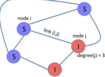
graph, each of the links is defined by a couple of nodesi,j∈V, and is denoted by(i,j)meaning that the nodesiand jare connected, see Fig 2.1. In this thesis, as mostly the case in the complex

network literature, we only deal with undirected simple networks which do not contain loops, i.e.

links from a node to itself, nor multiple links, i.e. couples of nodes connected by more than one

link.

Both the nodes and links can be associated with additional variables, such as node states or

link weights. For example, nodes could be assigned with one of two labelsSorIrepresenting

susceptible and infected nodes in a network where epidemic is spreading. Links in this example

could be assigned with a weight corresponding to the frequency of interactions which can pass a disease between the two nodes connected by the link. In the following we discuss some of the

main statistical properties used to characterise the structure and behavior of networked systems.

I  

S  

node  i  

node  j   link  (i,j)  

I  

S  

S  

degree(j)  =  3  

Figure 2.1:Schematic illustration of an undirected network with N=5 nodes, three of which are inSstate (susceptible) and two are inI state (infected).

2.1.1

Degree distribution

The degreek_iof nodei∈V is its number of connections, see Fig 2.1. The most basic topological

characterisation of a graph can be obtained in terms of the degree distribution, p_k, defined as

the probability that a node chosen uniformly at random has degreek or, equivalently, as the

fraction of nodes in the graph having degreek. The degree distribution offers a simple means to separate networks into classes. For example, many real networks, such as WWW [22, 49],

collaboration networks [20, 170] and cellular networks [134, 135], have been shown to display

power law degree distribution p_k ∼k−λ with a scaling exponent between 2≤λ ≤3. Thus,

unlike homogeneous networks such as regular lattices or random graph, these networks, having

a highly inhomogeneous degree distribution, result in the simultaneous presence of a few nodes

(the hubs) linked to many other nodes, and a large number of poorly connected elements. Such

networks have been named scale-free networks, because power-laws have the property of having

power  grid  

exponen,al  decay  

Pr

ob

ab

ili

ty

 d

is

tr

ib

u,

on

#  transmission  lines  

10-­‐4   10-­‐3   10-­‐2   10-­‐1   100  

1   _{10   100}  

WWW  

power-­‐law  decay  

10-­‐8   10-­‐6   10-­‐4   10-­‐2   100  

#  URLs  

1   ₁₀1   ₁₀2   ₁₀3   ₁₀4  

Figure 2.2:Degree distribution of the electric power grid of Southern California (figure adapted from [16]) and a network of documents connected by URLs obtained from the complete map of the nd.edu domain (figure adapted from [22]). Power-law distribution is characterised by a straight line in a log-log plot, thus also called scale-free distribution. The exponential decay observed in the power grid network is common in networks where constraints such as space and energy are preventing the formation of extremely high-degree nodes [16].

A very interesting property of scale-free networks, and even networks where the power law

behaviour holds only in the tail, is that if the scaling exponent of the degree distribution is in the

range 2<λ ≤3, then in the limit of large network size (N →∞), its first moment (i.e. mean

degree) is finite, while its second moment (related to the dispersion of the degree distribution)

diverges [176]. Suppose we have degree distribution, p_k, that has a power-law tail fork≥kmin.

Then, itsmth moment is given by

hkmi=

kmin−1

∑

kmp_k+C ∞

∑

km−λ

| {z }

pk=Ck−λ

'

kmin−1

∑

kmp_k+C Z ∞

kmin

= kmin−1

∑

kmp_k+ C

m−λ+1[k

m−λ+1_]∞

kmin (2.1)

The first term is a finite number and the second term diverges for m−λ+1≥0. Thus, for

2<λ ≤3, we obtain that the first moment is finite and the second moment diverges.

2.1.2

The small-world effect

The distancebetween two nodesi,j∈V,d_{i j}, is defined as the number of links in the shortest path from one node to the other (if there is any). The maximum value ofd_{i j} is called thediameter

of the graph, denoted byDiam(G). A measure of the typical separation between two nodes in

the graph is given by the average shortest path length, also known ascharacteristic path length,

defined as the mean distance over all couples of nodes

L= 1

N(N−1)_i,j∈V

∑

In regular d-dimensional lattices, the average path length grows with the lattice size as L∼

N1d [42]. In contrast, in most of the real networks, despite their often large size, there is a

relatively short path between any two nodes. This property is known as the “small-world” effect

and is mathematically characterized by slow scalingL∼lnN [241]. Another related notation

is the “six degrees of separation”, which refers to Milgram’s experiments, where a path of first-name acquaintances with a typical length of about six was found between most pairs of

people in the United States [157, 240].

But, although found in various types of real networks [241], including biological and

technologi-cal ones, the small-world effect does not imply a particular organisation principle, rather it is

an obvious mathematical property in some network models, including totally random networks

obtained by randomly placing links among a given number of nodes, which will be introduced in

section 2.2.1. Scale-free networks are considered “ultra-small”, since their characteristic path length scales even slower with the system sizeL∼ln lnN [68].

2.1.3

Clustering

In contrast to random graphs, the small-world property in real networks is often associated with

the presence ofclustering, meaning that in social networks, for instance, two friends of someone

are often also friends with each other. This is property can be quantified by the clustering

possible number of links [241]

C_i= 2Ei

k_i(ki−1)

(2.3)

wherek_iis the degree of nodei(i.e. number of friends), ki(ki−1)

2 is the maximum number of links

possible among the neighbours of nodei, andE_icounts how many of these links actually exists

(i.e. how many friends of nodeiare also friends with each other). The clustering coefficient of

the whole network is the average of all individualC_i’s.

An alternative measure, calledtransitivitymeasures the fraction of triples that have their third

link filled in to complete the triangle

T = 3 x number of triangles in the network

number of connected triples of nodes (2.4)

In other words,T measures ratio of the means, rather than the mean of ratios, giving less weight

to contributions of low-degree nodes [169].

Regardless of which definition, most real networks exhibit a significant amount of clustering

compared to random networks with the same number of nodes and links [169]. Moreover, it is

suspected than real networks have a nonzero clustering limit when the network becomes infinitely

large, so thatC=O(1)asN→∞, in contrast to random networks whereC=N−1[10].

2.1.4

Giant component

A connected component of a network is a maximal subset of nodes that are connected by paths through the network. The size of the largest connected component is an important quantity, and

in the limit of large network size (N→∞) is equated with thegiant componentwhich contains a

constant fraction of nodes of an infinite network. The existence of a giant component indicates

that most nodes in the networks,O(N), are reachable from one another, such that a rumour, for

example, could spread from one person to almost everyone else, unlike in networks composed of

many small components, not connected to one another (i.e. no giant component exists), where

the rumour could only spread within each component separately without invading the network

“globally”. Since one isolated node with no links is already enough to make a network not

connected (a connected network is one in which all nodes are connected to one another), the existence of a giant component is an important statistical property used to measure connectivity

2.2

Network models

In this section we present some of the main network formation models aim at generating specific

topologies that reproduce observed statistical features of real-world networks.

2.2.1

The Erd˝os-Rényi model

The classical Erd˝os-Rényi (ER) model of random graphs generates a random undirected network

withNlabeled nodes connected byMedges, which are chosen randomly from theN(N−1)/2 possible edges [89, 90]. The random graph ensemble with exactly N nodes and M links is sometimes denoted asG(N,M), forming a probability space in which every realisation out of the possibleC_NM_(N−1)/2is equiprobable.

An alternative and equivalent definition of a random graph, which is easier to analyse

mathematically, is the binomial model,G(N,p), where every pair of nodes being connected with probability p. Since the presence or absence of edges is independent, the resulting network has

Poisson degree distribution with meanz=p(N−1)

p_k=

N−1

k

pk(1−p)N−1−k' z

k_e−z

k! (2.5)

with the last approximate equality becoming exact in the thermodynamic limit of largeN and

fixedz[169].

The structural properties of ER random graphs vary as a function of p, showing, in particular, a

phase transition at a critical probability p_c= _N1 above which an extensive (i.e.,O(N)) fraction

of all nodes are joined together in a single giant component (see section 2.1.4), and the rest

of the nodes occupying smaller components with exponential size distribution and finite mean

size [42, 169]. This result will be discussed in detail in section 2.3.1, where we present site and

bond percolation processes.

ER random graphs are small-worlds - almost all graphs with the sameNand phave precisely the

same diameter concentrated aroundDiam=ln_lnN_z, and characteristic path length behaves the same

L∼ ln_lnN_z [11]. However, in almost all other respects, random graphs do not reproduce typical

features of real-world networks such as a scale-free degree distribution or strong clustering. Due

to the independent placement of links, they have clustering coefficientC=pwhich tends to zero

asN−1in the limit of large system size. Nonetheless, ER random graphs are an attractive baseline

model for various applications. Their simplicity makes them easy to analyse mathematically,

and more importantly, they constitute the basic building blocks of network theory, and our

2.2.2

Watts-Strogatz small-world networks

In order to capture the observed strong clustering in real networks together with short path

lengths, Watts and Strogatz (WS) generated a network interpolating between a regular graph and

a random graph [241], see Fig 2.3. Starting with a ring lattice withN nodes in which every node is symmetrically connected to itsm(m/2 on either side) nearest neighbors for a total ofM= mN₂

edges, create shortcuts by randomly rewire each link of the lattice with probability psuch that

self-connections and duplicate edges are excluded.

For p=0 we have a regular lattice with characteristic path lengthL(0)' ₂N_m 1 and clustering

coefficientC(0)' 3

4. On the other hand, for p=1 the model produces a random graph with

L(1)∼lnN

lnm andC(1)∼

m

N. For intermediate values of pbetween these limits, Watts and Strogatz

found an interval whereL(p)is close toL(1)yetC(p)C(1), thus producing a network with both the small-world property and a non-trivial clustering coefficient [11].

Figure 2.3:Construction of the Watts-Strogatz small-world model: interpolation between a regular graph

(p=0) and a random graph (p=1). Watts and Strogatz showed that for intermediate values of p, the

obtained network has both a small characteristic path length and a high clustering coefficient. Figure adapted from [241].

2.2.3

Barabási-Albert preferential attachment model

Both the ER and the WS model discussed above produce networks with narrow degree

distributions (see Fig. 2.4), unlike most real-world networks (see section 2.1.1). The

Barabási-Albert (BA) model [21] overcomes this flaw while attempting to provide an explanation to the

origin of the highly skewed degree distributions of real-world networks. The model incorporates

two essential ingredients, growth and preferential attachment, to produce scale-free networks.

is added to the network. The new node connects to nodes already present in the network with

probability proportional to their degree, i.e. according to linear preferential attachment. This

model has been shown to produce a network with degree distribution p_k∼k−3in the limit of

large networks [11]. The characteristic path length is smaller than in ER networks with the

same number of nodes and links [11], and has been shown to scale with the number of nodes

L∼ lnN

ln lnN[45]. The clustering coefficient decays slower than in random graphsC∼N

−0.75_{, but}

still vanishes with the system size.

Substituting the linear preferential attachment with sub-linear, super-linear or constant attachment

probability, has been shown to produce networks which are no longer scale-free [141], thus

suggesting that linear preferential attachment is essential to the formation of scale-free networks.

But Barabási and Albert were not the first to point this out. Already in 1965, Derek de Solla

Price found that citation networks have power-law degree distributions [79], and consequently

developed a model where the probability that a new published paper cites a previous one is taken

to be proportional tok_in+1, wherek_in is the number of times that the paper has already been

cited [190]. Price’s model itself is built on ideas developed in the 1950s by Herbert Simon, who showed that power laws, which appear in a wide range of empirical data, arise when “the rich get

richer” [212]. However, Barabási and Albert were the first to realise the enormous potential of

the model and its relevance for a wide range of real-world networks. Moreover, having neglected

the direction of links and fixing the number of links added with each new node, the BA model is

simpler than the one proposed by Price and is thus more intuitive and attractive. For that reason,

the preferential attachment model is usually referred to as the BA model.

2.2.4

Configuration model

The configuration model, introduced by Bender and Canfield [36], is a generalisation of the ER

random graph model, which allows to generate graphs with arbitrary degree distributions. Given

a degree sequenceD={k1,k2, . . .kN}, each nodeiis attached withki“stubs" sticking out of it,

which are the ends of links-to-be. Then, the graph is constructed by randomly choosing pairs of stubs and connecting them together. This procedure generates, with equal probability, every

possible topology of a graph with the given degree sequence [161]. Dis chosen in such a way

that the fraction of nodes with degreekwill tend to the desired degree distribution for largeN,

for example, by drawing a random sample from the degree distribution. The obtained graphs

may have loops and multiple links, but these can be neglected or discarded in the large network

limit,N→∞.

The configuration model is widely used to generate random uncorrelated networks, especially

study analytically. For example, the exact condition for the existence of a giant component and

its expected size was provided by Molloy and Reed [161, 162]. Newman et al. [175] studied the

average size of non-giant components, and Chung and Lu [132] studied the average distances

between nodes.

SF  (λ  =  2.5)  

BA  

WS  (p  =  0.1)  

ER  

k,  degree   p(k)  

0 0.1 0.2 0.3 0.4 0.5 0.6

0 5 10 15 20 25 30 35 40

ER BA WS (p=0.1) SF (h=2.5)

0 0.0002 0.0004 0.0006 0.0008 0.001

20 40 60 80 100

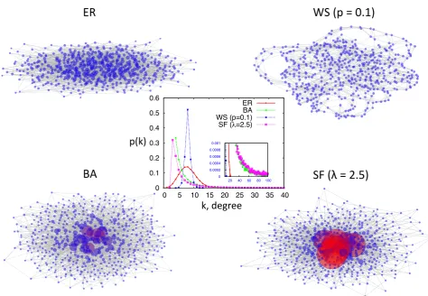
Figure 2.4:Visualisation of random networks withN=500 nodes and mean degreehki=8, obtained

through the ER model, WS model withp=0.1, BA model, and the configuration model using a degree

sequence drawn from a scale-free degree distribution with scaling exponentλ =2.5. Nodes sizes and

colours correspond their degree. The graph in the middle shows the obtained degree distributions for

larger graphs (N=100 000) generated in the same way. As expected, the degree of nodes in the WS

2.3

Dynamics on networks

As described in the previous two sections, network science initially revolved around developing

quantitative tools to characterise the structure of real-systems, following by the development of

network formation models which generate their observed statistical features. With the advances

in our understanding of their complex structure, the focus of network science has turned to

investigate the implications of such structures to the behaviour and functionality of networked dynamical system. This still remains the ultimate goal and thus the main focus of network

science, and in the following, we describe the two most important and widely used models of

networks dynamics, which are also repeatedly used throughout this thesis.

2.3.1

Percolation and network resilience

One of the first examples to be studied thoroughly of a process taking place on a network has

been site and bond percolation processes. A site (bond) percolation process is one in which

nodes (links) are removed from the graph withfailure probability f. The probability to remain in

the graph, p=1−f, is often called theoccupation probability, since we could think of removed

nodes (links) as “unoccupied” (i.e. nonfunctional or nonoperational), and the remaining nodes

(links) as “occupied”.

When the occupation probability is small, the network is composed of a large number of very

small connected components, unreachable from each other through occupied nodes. But as the

occupation probability increases, it reaches a critical value, p_c, called thepercolation threshold,

above which a giant component emerges, connecting a positive finite fraction of the nodes in the

network [46]. The percolation threshold can be used as a measure for network resilience - the

smaller it is the more robust is the network since a small fraction of occupied nodes is already

enough for the giant component to emerge, i.e. to have global connectivity.

One of the most interesting results in the study of complex networks is that infinitely large

networks with power-law degree distributions p_k ∼k−α for some constant 2≤α ≤3 have

a critical value p_c=0, indicating that the network always has a giant component, or in the

language of physics, the network always percolates [67]. To gain a better understanding of this

striking results, in the following we present the generating functions approach developed by

Newmanet al.[175] to analytically study a site percolation process on random networks.

2.3.1.1 Generating functions

Consider a random graph with a large number of nodes,N, and structure of the configuration

identically distributed from some degree distribution p_k, and are randomly connected with the

only constraint that a node with degreek has exactlyklinks. The generating function of the

degree distributionp_k is a power series whose coefficients are the degree probabilities p₁,p₂, . . .

G₀(x) = ∞

∑

p_kxk (2.6)

where|x| ≤1, and the distributionp_k is assumed correctly normalized, so thatG₀(1) =1.

Generating functions are an extremely powerful tool in combinatorial enumeration problems

allowing us to use functional manipulations to study, for example, the average number of nodes

in a network component [244]. In the following we review some of their properties that will prove useful in subsequent development, and especially in chapter 3. First, we observe that the

generating functionG0given in 2.6 indeed “generates” the probability distribution pk, meaning

that givenG₀, we can retrieve the component probabilities of p_k. The probability that a node has

kconnections is given by thekth derivative ofG₀according to

p_k= 1

k! dkG₀

dxk |x=0 (2.7)

The next useful property of the generating function is that we can use it to extract summary

statistics directly. The mean of the distribution, which corresponds to the mean degree,hkiis

given by

hki=

∞

∑

k p_k=G0₀(1) (2.8)

Higher moments of the distribution can be calculated from higher derivatives also, and in general,

we have

hkni=

∞

∑

knp_k=

h

x d

dx

n G₀(x)

i

x=0 (2.9)

Finally, generating functions have a “powers” property, that if the distribution of a propertyα

of an object is generated by a given generating function, then the distribution of the total ofα

summed overm independent realizations of the object is generated by themth power of that

generating function. For example, the distribution of the sum of the degrees ofmnodes chosen

at random from a network with degree distribution p_k, is generated byG₀(k)m[175].

We continue by defining the generating function for the excess degree distribution defined as follows. Consider the probability of following a randomly selected link to reach a node with

an additional k links, apart from the one by which it has been reached. This probability is

(which makes itk+1 times more likely to be arrived at than a 1 degree node). Therefore, the

distribution of the remaining degrees of nodes reached by following a random link, called the

excess degree, isq(k) = (k+∞1)p(k+1)

∑ k=1

k p(k)

and the associated generating function is given by

G1(x) =

∞ ∑ k=0

(k+1)pk+1xk

hki =

1

hkiG0

0_(x).

(2.10)

2.3.1.2 Connected components

Let us now consider the distribution of the sizes of connected components in the graph. Let

H₁(x)be the generating function for the distribution of the sizes of components that are reached

by choosing a random link and following it to one of its ends. Note that the giant component, if there is one, is excluded fromH1(x). Thus, component sizes are finite and the chances of a

component containing a closed loop of links goes asN−1which can be neglected in the limit of

largeN. In other words, each component is treelike in structure, consisting of the single nodev,

we reach by following our initial link, plus any number plus (including zero) of other treelike

components, with the same size distribution, joined to it by single links. Summing over all the

types of connectivity possible forvleads to the self consistency equation forH₁(x)

H₁(x) = x q₀

|{z}

nodevhas no additional links

+ x q₁H₁(x)

| {z }

nodevhas 1 additional link

+ x q₂[H1(x)]2

| {z }

nodevhas 2 additional link

+. . . (2.11)

However,q_k is nothing other than the coefficient ofxk in the generating function G₁(x), see

equation 2.10, and hence equation 2.11 can also be written

H₁(x) =xG₁(H1(x)). (2.12)

Starting from a randomly chosen node, rather than link, we have one such component at the

end of each link leaving that node, and hence the generating function for the size of the whole

component is

H₀(x) =xG₀(H1(x)). (2.13)

Using the equations developed above we can now find properties of interest such as the mean

component size to which a randomly chosen node belongs. According to Eq. 2.8, this quantity

can be extracted from the generating function for the distribution of components sizes according to

From equation 2.12 we have

H10(1) =1+G10(1)H10(1) (2.15)

and by substituting into equation 2.14 we obtain

hsi=1+ G0

0₍₁₎

1−G₁0(1). (2.16)

The point where the average component diverges, G₁0(1) =1, marks the phase transition at

which a giant component first emerges. This yields a critical occupation probability, above

which the giant component exists, p_c= _G1 10(1) =

hki

hk2_i, wherehk

2_{iis the second moment of the}

degree distribution p_k. Therefore, in scale-free networks where the first moment is finite and

second moment diverges in the limit of large network (see equation 2.1),p_cgoes to zero with the

network size, i.e., the network contains a giant component when any finite fraction of the nodes or links are removed.

At the point where the giant component first emerges,H₀(1)is no longer unity (since it excludes

the giant component) but is equal to 1−S, whereSis the fraction of nodes in the giant component.

Thus, we obtain

S=1−H₀(u) =1−G₀(H₁(u)) (2.17)

whereu≡H₁(1)is the smallest non-negative real solution of

G₁(u) =u (2.18)

since by definitionu=H₁(1) =G₁(H1(1)) =G1(u).

2.3.1.3 Attack tolerance

Finally, we would like to briefly discuss the extension of Callawayet al.[57] to the approach

presented here. In their method, the occupation probability is no longer fixed across the network,

but instead it is a function of the degree of nodes. Letr_kbe the occupation probability of a node

with degreek. We define the generating functions for the distribution of the degree and excess

degree of occupied nodes:

F₀(x) = ∞

∑

p_kr_k xk, F₁(x) = F 0

0(x)

Then, the probability distribution of the size of the component of occupied nodes to which a

randomly chosen node belongs is generated byJ₀(x), where

J0(x) =1−F0(1) +xF0(J1(x)), J1(x) =1−F1(1) +xF1(J1(x)) (2.20)

and the mean component size is given by

hsi=F₀(1) +F0 0_(1)F

1(1)

1−F10(1)

. (2.21)

Once the giant component emerges, which happens atF10(1) =1, its size is given by

S=F₀(1)−F₀(u), u=1−F₁(1) +F₁(u) (2.22) Using this approach, Callawayet al.[57] studied the resilience of networks to attack in which

nodes are removed in order from highest degree to lowest degree, and confirmed previous

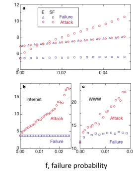
numerical studies showing that scale-free networks are highly susceptible to this kind of attack, much more than networks with narrow degree distributions such as ER networks [13, 49], see

Fig. 2.5. We further demonstrate an application of this approach to study attacks in multiple

networks in chapter 3.

2.3.2

Epidemic spreading

The second set of processes that have been widely investigated, together with bond and site

percolation described above, is epidemiological processes. Here we are interested in what are the

network topologies that give rise to disease, information, and rumour spreading over them. We

begin by describing the two most studied models in epidemiology, susceptible-infected-recovered

(SIR) and susceptible-infected-susceptible (SIS) models of epidemic disease [17, 19, 124]. The

SIR model describes diseases resulting from permanent immunisation or death of infected

individuals. In this model, each individual can be in one of three possible states: (S) susceptible corresponds to healthy individuals who do not have the disease but can catch it if exposed to

infected individuals, (I) infected corresponds to individuals who have the disease and can pass it

on, and (R) recovered or removed corresponds to individuals who recovered from disease and

have permanent immunity, or individuals who died from the disease, and they can never get it

again or pass it on. The SIR model has been shown to describe diseases such as chickenpox,

HPV, seasonal influenza, and H1N1 [17, 70], as well as rumour-spreading [164, 247] and the

spread of computer viruses [150]. It is based on two parameters, infection rate,β (i.e. infection

D

,  d

iam

ete

r  

f,  failure  probability  

Figure 2.5:Robustness of scale-free (SF) and exponential (E) networks to attack and random failure. As demonstrated using both random networks models (a) and real-world networks (b)-(c), scale-free networks are extremely resilient to random nodes failure, where the network diameter is almost unaffected in the range shown. However, the diameter of scale-free networks is increasing very rapidly when attacking nodes in order from highest degree to lowest degree, much more than exponential networks. Figure adapted from [13].

rate,γ, in which infected recover and become immune to the disease. Under the fully mixed

assumption, where one assumes that any susceptible can catch the disease from any infected (i.e.

individuals they make contact with are randomly chosen from the whole populations), the time evolution of the disease is given by

ds

dt =−βis, di

dt =βis−γi, dr

wheres,i, andris the fraction of susceptible, infected and recovered individuals respectively.

In other words, s,i, andr is the probability that a node is susceptible, infected or recovered

respectively, and therefore multiplying generates the compound probability of having both in

any pair chosen at random, with full mixing guaranteeing no bias in terms of node adjacencies.

In some spreading processes, individuals (or other entities such as computers) can catch the

same disease more than once, and thus in the SIS model, infected individuals recover in rateγ and become susceptible again, describing diseases such as tuberculosis, gonorrhea and common

cold [17, 19, 124], as well as computer viruses in systems with no automatic updated antivirus

programs [183, 184]. Again, under the fully mixed assumption, the time evolution of a SIS

spreading process is given by

ds

dt =−βis+γi, di

dt =βis−γi (2.24)

The most important point is that the dynamical equations of both SIR and SIS always yields

a non-zero epidemic threshold (also called basic reproduction number) corresponds to critical

infection rate above which the disease persists (in case of SIS), or the disease spreads and infects

a non-zero fraction of the population in the limit of large system size (in case of SIR).

But unlike the fully mixed assumption, in reality, diseases can only spread between people who

have physical contact. Therefore it is important to consider the structure of the contact network, especially in cases like sexually transmitted diseases where there is a large heterogeneity in

degrees of sexual activity within the overall population [17, 19, 124]. When a disease is spreading

over a network, individuals, represented by nodes, can only catch the disease from their network

neighbours. Thus, moving from differential equations to processes over a network allows

us to consider the structure of interactions, which is otherwise neglected by the fully mixed

assumption. Grassberger showed that SIR spreading over a network can be mapped exactly onto

bond percolation on the same network [111]. Then, the percolation threshold corresponds to

the epidemic threshold; the distribution of percolation clusters (i.e., components connected by

occupied links) corresponds to the distribution of the sizes of disease outbreaks that start with a randomly infected node; and the size of the giant component corresponds to the size of the

epidemic outbreak. Therefore, the result discussed in section 2.3.1, where scale-free networks

with scaling exponent 2≤λ ≤3 always percolate, means that in these networks there is no

non-zero epidemic threshold. In other words, diseases will always propagate in these networks,

regardless of the infection and recovery rates [153].

Although the SIS model cannot be solved exactly on a network as can the SIR model,

equations [183, 184]. In short, the idea is to allow the rate of infection to vary among nodes

based on their degree, replacingiandswithi_kands_krepresenting the fraction of nodes of degree

kthat are infected or susceptible. The advantage of this approach is that it can tell not only the

long time behaviour of the outbreak (e.g. finial outbreak size, critical infection rate), but also

the time evolution of an outbreak. Pastor-Satorras and Vespignani showed that also in the SIS

case, where the network has power-law degree distribution with scaling exponent 2<λ ≤3, the disease will never die out regardless of the infection and recovery rates.

Obviously, real systems are always finite and thus even in scale-free networks there is always an

effective non-zero epidemic threshold, below which the epidemic will not spread. In addition,

scale-free networks with high clustering coefficients [88], as well as networks embedded in

regular Euclidean space [197, 237], have also been shown to exhibit non-zero epidemic thresholds.

But although the absence of non-zero epidemic threshold does not hold in various types of

systems, scale-free networks are still proved to be very good spreaders. For example, it has been

shown that the epidemic threshold scales with system size asβ(N)∼ _ln1_N and is therefore very

small even for not very large networks, and is significantly smaller than that of a random graph with the same size [185]. Therefore, various immunisation strategies on scale-free networks have

been examined [17, 81, 186]. Uniform immunisation has been shown to be totally ineffective on

scale-free networks, since it depresses the infection prevalence too slowly, and thus, in the limit

of infinite system size, the critical fraction of nodes to immune such that an epidemic will not

break is one, i.e. all nodes need to be vaccinated. But even for finite systems, unrealistically high

densities of randomly immunised individuals are required to stop the epidemic from breaking.

However, targeted immunisation based on the node connectivity is highly effective and can

potentially eradicate a virus.

And fortunately, there is even an easy way to find high-degree nodes without global knowledge

of the network, which is very important in cases like sexual contact networks, where it is hard to

obtain data. Cohenet al.[69] have pointed out that the probability of reaching a particular node

by following a randomly chosen link is proportional to the nodes degree (see excess degree in

section 2.3.1). Therefore, by choosing a random person from a population and vaccinating one of

their friends, an efficient targeted immunisation can be achieved. And in fact, the “contact tracing”

method, that has been widely effective in controlling STDs [65, 95] and SARS [149, 193], is

2.4

Coupled networks

The exploding body of work that has been described in previous sections is providing a firm

basis to the evolution of network science. The major challenge at this point is to account for

more realistic features of networks such as strong coupling between networks (networks are not

isolated), the time evolution of networks (networks are not static), the coevolution of structure

and dynamics (structure is affected by dynamics), other classes of links including different signs of interactions, and spatial properties including geographical aspects of networks [122].

And indeed, in recent years there has been a great effort to tackle some of these challenges. For

example, while most of the studied until now assumed that networks are not changing over time,

or that the time-scale of structural changes is much slower than the dynamics taking place, the

emerging topic of temporal networks is examining networks where links are generated, disappear

and reappear over time, developing methods for analysing topological and temporal structure

and models for explaining their relation to the behavior of dynamical systems [126].

Adaptive networks, combining dynamics on a network with dynamical adaptive changes of the

underlying network topology have only recently started to get attention [115, 116]. Examples

include social networks where links with ill people (dynamics) might be temporarily removed

(structure) in order to avoid infection, or repeating traffic congestions (dynamics) on a given road

could lead to formation of new roads (structure). In these networks, a feedback loop between the

state and topology of the network is formed, giving rise to a remarkably rich dynamical behaviors,

which are very difficult to study analytically. We will expand on this topic in chapter 4.

Different types of interactions between entities in a system, such as negative and positive social

links [147], as well as dependency links representing strong local relations [181], have been

recently suggested explaining social phenomena and dynamics that could not be addressed

before.

Finally, research on spatial networks aims to understand how the spatial constraints affect the

structure and properties of networks which are embedded in space, such as the Internet, mobile

phone networks, power grids, and neural networks [26].

But undoubtedly, the topic that has been getting most attention since the revolutionary paper

of Buldyrev et al. [53] that was published in 2010, is coupled multilevel networks. Both

natural and engineered systems are rarely isolated. They interact with the environment and

one another constituting a part of a much larger complex multilevel system. Such examples include people involved in more than one social network [238], proteins in a cell interacting

and critical infrastructures depending both on one another [195] and on political and social

processes [61]. As technology has advanced, the coupling between individual networks, that

were treated as isolated systems until now, is becoming stronger and stronger. Aside from

physical, logical and geographical interdependencies, most systems today, including critical

infrastructures such as power-grids, exhibit cyber-dependency, where normal functioning relies

on information technology [194, 195, 234].

And the reason that these strong couplings and interdependencies are attracting so much attention,

is that they seem to give rise to completely new phenomena, that have never been observed in

isolated single networks. Havlinet al.[122] compares this paradigm shift from single networks

to coupled multilevel networks, to the interactions between particles in physics: “As in physics,

when only the individual particles were studied it was made possible to understand the properties

of gas; however, when the transition was made to study the interactions between these particles,

it was finally made possible to understand and describe liquids and solids. Thus, such a transition

in network science will lead to a significant paradigm shift, which will reveal a multitude of new

features and phenomena.”

2.4.1

Interdependent networks

In an attempt to provide a mathematical framework for analysing the consequences of cascades

of failures occurring in interdependent critical infrastructures [194, 195], Buldyrevet al.[53]

defined a new class of networks calledinterdependent networks, and studied a percolation process

in a system of two interdependent networks. In these networks, unlike the connectivity links

within each networks, the networks are interconnected bydependency links, representing the fact

that the function of a given node in one network depends crucially on nodes in other networks.

Thus, when a node from one network is removed in a percolation process, its dependent node

from the other network is automatically removed as well.

This model was designed to capture the situation observed in real-world data from a power

network and an Internet network (a supervisory control and data acquisition system). The data

was extracted from an electrical blackout that affected much of Italy in 2003, where the shutdown

of power stations directly led to the failure of nodes in the Internet communication network

(since switches rely on electricity), which in turn caused further breakdown of power stations

(since they rely on the Internet for control and recovery) [195].

In their model, Buldyrevet al. consider two equal size networks with arbitrary degree distribution,

where each node from one network is mutually dependent on a randomly selected node from

are significantly more vulnerable than their non-interacting counterparts, where small failure

in one network may lead to catastrophic consequences that breaks the whole system. This

behavior is characteristic of a first-order phase transition, in contrast to the second-order

phase transition characterising percolation of a single network, where the size of the giant

component is decreasingcontinuouslyas the number of removed nodes increases, see Fig. 2.6.

Here, instead, when a critical number of nodes are removed, the giant component suddenly

(i.e. discontinuously) collapses, resulting in a first order percolation transition. Perhaps more

importantly that the qualitative change in the percolation transition, the authors show that in contrast to single networks, interdependent networks with broader degree distributions are more

vulnerable. Specifically, the result where single scale-free networks always percolate in the limit

of large networks (see section 2.3.1), is no longer valid for interdependent scale-free networks.

p,  occupa(on  probability  

S,

 s

ize

 o

f  l

ar

ge

st  

co

m

po

ne

nt

0  

0.5  

1  

0  

0.2  

0.4  

0.6  

0.8  

1  

second  order  

first  order  

p,  occupa(on  probability  

0  

0.5  

1  

(a)   (b)  

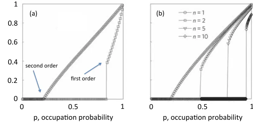
Figure 2.6:Second order vs. first order percolation transition. (a) In two weakly interdependent networks (with few interdependency links between them), the size (fraction of nodes) of the largest connected component is changing continuously with the fraction of occupied nodes in the network. However,

in strongly interdependent networks, the transition is discontinuous “jumping” from 0 to≈0.4 at the

percolation threshold. In other words, the giant component suddenly forms in this case, where in weakly

interdependent networks it forms gradually. (b)nfully interdependent networks (all nodes mutually

depend on nodes in other networks). As the number of networksnincreases, the “jump” in the size of the

largest connected component is bigger. Figure adapted from [103].

As stated earlier, the model of Buldyrev et al. has attracted considerable attention and

consequently has been extended in various ways [103]. For example, in a system of two