Generalized Eulerian Numbers

(1)

http://www.scirp.org/journal/apm ISSN Online: 2160-0384

ISSN Print: 2160-0368

Generalized Eulerian Numbers

Alfred Wünsche

Institut für Physik, Humboldt-Universität, Berlin, Germany

Abstract

We generalize the Eulerian numbers k

l to sets of numbers Eµ

( )

k l, ,

(

µ

=0,1, 2,

)

where the Eulerian numbers appear as the special case

µ

=1.

This can be used for the evaluation of generalizations Gµ

( )

k z; of the

Geometric series G0

( )

k z; =G1

( )

0;z by splitting an essential part

(

)

( 1)

1−z −µk+ where the numbers E_µ

( )

k l, are then the coefficients of the

remainder polynomial. This can be extended for non-integer parameter k to the approximative evaluation of generalized Geometric series. The recurrence relations k→ +k 1 and

µ

→ +

µ

1 for the Generalized Eulerian numbers

are derived. The Eulerian numbers

E k l

1

( )

,

are related to the Stirling numbers of second kind S k l

( )

, and we give proofs for the explicit relations

of Eulerian to Stirling numbers of second kind in both directions. We discuss some ordering relations for differentiation and multiplication operators which play a role in our derivations and collect this in Appendices.

Keywords

Eulerian Numbers, Eulerian Polynomials, Stirling Numbers,

Permutations, Binomials, Hypergeometric Functions, Geometric Series, Vandermonde’s Convolution Identity, Recurrence Relations, Operator Orderings

1. Introduction

The Eulerian numbers are discussed in the remarkable monograph of Riordan [1] from a combinatorial view and are the special topics in the recently published voluminous and versatile monograph of Petersen [2] with huge material and relations to other topics and with a great number of citations. The last contains How to cite this paper: Wünsche, A.

(2018) Generalized Eulerian Numbers. Advances in Pure Mathematics, 8, 335-361. https://doi.org/10.4236/apm.2018.83018

Received: February 12, 2018 Accepted: March 26, 2018 Published: March 29, 2018

http://creativecommons.org/licenses/by/4.0/

Open Access

(2)

also some remarks about the history of these numbers. The Eulerian numbers are taken into account in the article of Bressoud [3] in the NIST Handbook of Mathematical Functions [4]. In the interesting book of Conway and Guy [5], the “Eulerian numbers” are also shortly mentioned with one formula but without explicitly giving tables. There exist also an article about the Eulerian numbers in Weisstein’s Encyclopedia of Mathematics [6].

We met the Eulerian numbers A k l

( ) (

, , k=0,1, 2,;l=0,1, 2,

)

first in

quantum-mechanical calculations of some expectation values for coherent phase states and in cumulant expansions of the distance to an initial state in the time evolution of this state for the Hamiltonian of a harmonic oscillator [7]. To this time, we looked for references where these numbers which we calculated explicitly are present in literature and found them in the monograph of Riordan [1] about combinatorics1_{. Meanwhile, there appeared the already mentioned} monograph of Petersen [2] which provided us a convenient access to this topics.

Bressoud and Petersen denote the Eulerian numbers by k

l similar to the

binomial numbers k

l    

  and likely based on earlier sources. The Eulerian

numbers may be ordered in form of a triangle (Eulerian triangle) in analogy to the Pascal triangle and with a similar palindromic symmetry. The notation of Petersen and of others [6] is related to the notation of Riordan [1] by

(

, 1

)

k

A k l

l = + but concerning the definition of k and l the first as it seems to

us is preferable and we denote it by 1

( )

,

k E k l

l

= since we generalize it to numbers Eµ

( )

k l, with arbitrary

µ

≥0.

The Eulerian numbers possess a combinatorial background although not introduced in this way by Euler [1][2]. They make a subdivision of the whole number of k! permutations of k elements in non-intersecting sets of permutations with the same number l of descents and what counted are the Eulerian numbers k

l . A descent in a permutation is present if from two

adjacent numbers in a permutation, the first is larger than the second. This explains why the sum of Eulerian numbers of k elements is equal to the total number of k! permutations and why the Eulerian numbers are symmetric with respect to descent and ascents.

As mentioned, in the present work we generalize the Eulerian numbers to sets of numbers Eµ

( )

k l, with interesting properties where the Eulerian numbers

1_{In the Russian translation of this monograph which we used they were translated as “Euler}

num-bers” but since these did not be the better known numbers which are usually understood under this name we called them “Eulerian numbers” without being aware that in English they are really called in this way.

(3)

are identical with our special case 1

( )

,

k E k l

l

≡ _{. Our primary intention was to}

obtain approximations in the evaluation of series from type of generalized Geometric series where the number k in Eµ

( )

k l, is not necessarily an integer

(Section 3). Such series with 1

2

k= appear in quantum optics for coherent phase states in the calculation of some kind of expectation values. We discuss some properties of the numbers Eµ

( )

k l, and derive the recurrence relations

for them. Furthermore, we find close relations between these numbers and the Stirling numbers of second kind. In Appendices, we discuss how some needed ordering relations for differentiation and multiplication operators are related with the Stirling numbers.

2. Introduction of Generalized Eulerian Numbers by

Evaluation of Generalized Geometric

Series

We present in this Section our concept of the introduction of Generalized Eulerian numbers E_µ

( )

k l, from the evaluation of generalized Geometric series

and give explicit results and tables but without the proofs which we develop in the following Sections.

The Geometric series as special case of the Hypergeometric Functions

(

)

1F0 a; ;− z (special case of general pFq

(

a1,,a cp; ,1,c zq;

)

(

)

(

)

(

₍

₎

)

(

)

1 0 0

1 0

0

1

F 1; ; , 1

1 ! 1

F ; ; .

1 ! ! 1

n

a n

z z

z

n a z

a z

a n z

∞

=

∞

=

= ≡ −

−

 _{+ −} 

 − ≡ = 

 − − 

 

∑

(2.1)

The convergence region of this series in the complex plane is z <1.

In our concept we consider the following types of generalizations Gµ

( )

k z;

of the Geometric series with index µ_{and with}_k_{as two parameters}

(

)

( )

(

)

(

)

( )

(

)(

)

(

)

(

)

( )

(

)(

)

(

)

(

)

( )

0

0 0

1

0 0

1 1

1

0 0

2

2 2

2 1

0 0

3

3 3

3 1

0 0

1

1 , ; ,

1

1 , ; ,

1

2 1 , ; ,

1

3 2 1 , ; ,

1

k n l

n l

k

k n l

k

n l

k

k _n _l

k

n l

k

k _n _l

k

n l

z E k l z G k z

z

n z E k l z G k z

z

n n z E k l z G k z

z

n n n z E k l z G k z

z

∞

= =

∞

+

= =

∞

+

= =

∞

+

= =

= ≡

−

+ = ≡

−

+ + = ≡

−

+ + + = ≡

−

∑



(2.2)

where G0

( )

k z; =G1

( )

0;z is the Geometric series.

The coefficients E_µ

( )

k l, in the expansion of the separated functions

( )

;

Eµ k z in powers of z are given by

(4)

( )

(

( )

(

)

( )

( ) (

₍

)

_{) (}

)

( )

( ) (

₍

)

_{) (}

(

)(

)

( )

( ) (

₍

)

_{) (}

(

)(

)

0 ,0 0 0

0

1

0

2

0

3

0

1 1!

, , , 0 1, , 0; 1, 2, ,

!(1 )! 1 1 !

, 1 ,

! 1 !

1 2 1 !

, 2 1 ,

! 2 1 ! 1 3 1 !

, 3 2 1 ,

! 3 1 !

j l

l j

j l

k

j j

l _k

j j

l _k

j

E k l E k E k l l

j j

k k

E k l l j

l

j k j

k

E k l l j l j

j k j

k

E k l l j l j l j

j k j

δ

=

−

= = = = =

−

− +

= + − ≡

+ −

− +

= + − + −

+ −

− +

= + − + − + −

+ −

∑





(2.3)

The numbers k

l here denoted by E k l1

( )

, are the Eulerian numbers. The

second of the relations (2.2) for G k z1

( )

; is called the Carlitz identity (Petersen [2], Equation (1.10 on p. 10) and the second of the relations (2.3) is the explicit sum representation of the Eulerian numbers ([2], Equation (1.11) on p. 12). The sequence of numbers E_µ

( )

k l, with

µ

=2, 3, represents a generalization of

the Eulerian numbers for integer parameter k but it is possible to extend it for non-integer k.

The generalization of (2.2) with integer indices

µ

=0,1, 2, is

( )

(

)

( )

(

)

1

(

)

1

( )

0 0

;

! 1

; , ,

! 1 1

k

n l

k k

n l

E k z

n

G k z z E k l z

n z z

µ µ

µ µ µ µ

µ

∞

+ +

= =

+

 

≡   ≡ ≡

− −

 

∑

(2.4)

with the polynomials E_µ

( )

k z; of degree µk or smaller

( )

(

)

( )

0 0

( ; ) , ; 1 , .

k k

l

l l

E k z E k l z E k z E k l

µ µ

µ µ µ µ

= =

≡

∑

⇒ = =

∑

(2.5)

Explicitly one finds for the coefficients E_µ

( )

k l, of these polynomials

( )

( ) (

₍

)

₎

(

₍

₎

)

0

1 1 ! !

, .

! 1 ! !

k j

l

j

k l j

E k l

j k j l j

µ

µ µ

µ

=

 

− + − +

≡ _ _

+ − _ − _

∑

(2.6)

The introduction of the functions Eµ

( )

k z; is connected with an evaluation

of the series G_µ

( )

k z; under separation of an essential part

(

1−z

)

−(µk+1) from

remainder polynomials Eµ

( )

k z; in z which could be called Generalized

Eulerian polynomials. In particular, this separation is effective for evaluations if z comes near to the boundary z =1 of convergence of the series.

We give now short tables (Tables 1-4) of the numbers E_µ

( )

k l, up to

µ

=3

which are easily to calculate by a computer:

In principle, the tables for

µ

≥2 could be reduced for the common factors !k

µ in the k-th line.

We have the following relations of the Eulerian numbers E k l1

( )

, to notations in [3][2] and in [1][5]

( )

(

)

1 , k l, 1 , 1 .

k

E k l A A k l

l +

≡ ≡ ≡ + _(2.7)

(5)

Table 1. Numbers E0

( )

k l, .

k l=0 l=1 l=2 l=3 l=4 l=5 l=6 l=7 l=8 l=9 0 0

( )

,

k

l=E k l

∑

0 1 0 0 0 0 0 0 0 0 0 1 = 0!

1 1 0 0 0 0 0 0 0 0 0 1 = 0!

2 1 0 0 0 0 0 0 0 0 0 1 = 0!

[image:5.595.59.539.103.430.2]

           

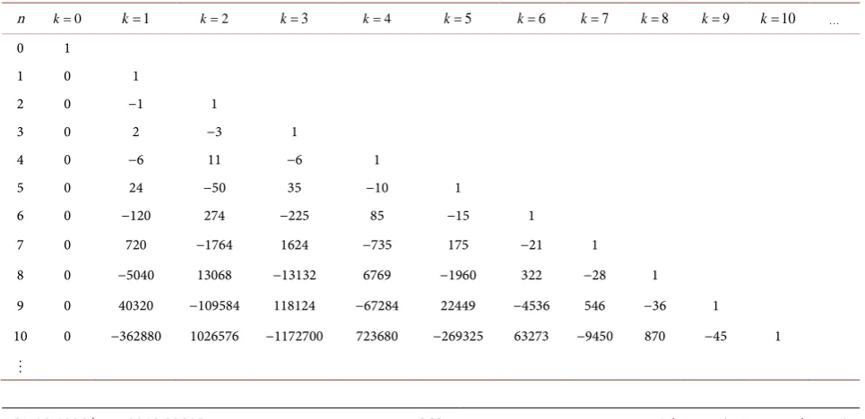
Table 2. Numbers 1

( )

,

k E k l

l

≡ (Eulerian numbers).

k l=0 l=1 l=2 l=3 l=4 l=5 l=6 l=7 l=8 l=9 0 1

( )

,

k

l=E k l

∑

0 1 0 0 0 0 0 0 0 0 0 1 = 0!

1 1 0 0 0 0 0 0 0 0 0 1 = 1!

2 1 1 0 0 0 0 0 0 0 0 2 = 2!

3 1 4 1 0 0 0 0 0 0 0 6 = 3!

4 1 11 11 1 0 0 0 0 0 0 24 = 4!

5 1 26 66 26 1 0 0 0 0 0 120 = 5!

6 1 57 302 302 57 1 0 0 0 0 720 = 6!

7 1 120 1191 2416 1191 120 1 0 0 0 5 040 = 7!

8 1 247 4293 15619 15619 4293 247 1 0 0 40 320 = 8!

[image:5.595.59.538.469.594.2]

9 1 502 14608 88234 156190 88234 14608 502 1 0 362 880 = 9!

Table 3. Numbers E2

( )

k l, (common factors 2!

k in the k-th lines).

k l=0 l=1 l=2 l=3 l=4 l=5 l=6 l=7 l=8 0 2

( )

,

k

l= E k l

∑

0 1 0 0 0 0 0 0 0 0 1 = 0!

1 2 0 0 0 0 0 0 0 0 2 = 2!

2 4 16 4 0 0 0 0 0 0 24 = 4!

3 8 160 384 160 8 0 0 0 0 720 = 6!

4 16 1152 9648 18688 9648 1152 16 0 0 40320 = 8!

[image:5.595.58.537.633.731.2]

5 32 7424 165056 885248 1513280 885248 165056 7424 32 3628800 = 10!

Table 4. Numbers E3

( )

k l, (common factors 3!

k in the k-th lines).

k l=0 l=1 l=2 l=3 l=4 l=5 l=6 l=7 l=8 0 3

( )

,

k

l=E k l

∑

0 1 0 0 0 0 0 0 0 0 1 = 0!

1 6 0 0 0 0 0 0 0 0 6 = 3!

2 36 324 324 36 0 0 0 0 0 720 = 6!

3 216 11 664 87 480 164 160 87 480 11 664 216 0 0 362 880 = 9!

(6)

The first line for k=0 in Table 2 is not written in [1][2] and then we have a triangle similar to the Pascal triangle and the notation k

l is chosen in analogy to the binomial coefficients k

l    

  in the Pascal triangle 2

(

)

0

( ) (

(

)

) (

)

1 1 ! !

, 1 .

! ! ! 1 !

j l

k

j

k k k k

l j

l l k l l = j k j

− +

 ₌ ₌ _{+ −}

  ₋ _{+ −}

 

∑

(2.8)

With the line to k=0 in Table 2 the Eulerian numbers E k l₁

( )

, form a triangle with an additional tip.

Similarly to the binomial coefficients in

(

1+x

)

k, from the Tables 1-4 we see

that the polynomials Eµ

( )

k z; are palindromical ones (for integer µ) with the

following relation for the coefficients E_µ

( )

k l, with fixed k

( )

,

(

,

(

1

)

,

(

0,1, 2,

)

,

E_µ k l =E_µ k

µ

k− −l k=  (2.9)

and for the coefficients in the first columns for l=0 one has

( )

, 0 ! .k

E_µ k =µ (2.10)

Obviously, as to see from (2.13) and from the tables, the numbers in all rows (fixed k) possess the common factor µ!k in their factorization that is 1!k =1

for the Eulerian numbers and in this sense the tables for E_µ

( )

k l, with

µ

≥2

could be simplified. For the sum of all coefficients Eµ

( )

k l, over l one finds

(

)

( ) ( )

0

; 1 , !.

k

l

E k z E k l k

µ

µ µ

µ

=

= =

∑

= (2.11)

Although the properties (2.9), (2.10) and (2.11) are evident from Tables 1-4 and can be affirmed by computer up to higher values as given they have to be proved that we make in the following Sections.

The integers k in the generalizations Gµ

( )

k l, of the Geometric series in (2.2)

can be extended to arbitrary real numbers k in the convergence region according to

( )

(

)

( )

(

)

1

(

)

1

( )

0 0

;

! 1

; , ,

! 1 1

k

n l

k k

n l

E k z

n

G k z z E k l z

n z z

µ

µ µ µ µ

µ

∞ ∞

+ +

= =

+

 

≡   ≡ ≡

− −

 

∑

(2.12)

where then the polynomials E_µ

( )

k z; make the transition to entire function

with the infinite sequence of coefficients Eµ

( )

k l; of their Taylor series given

by (2.13)

( )

( ) (

₍

)

₎

(

₍

₎

)

(

)

0

1 1 ! !

, , 0,1, 2, .

! 1 ! !

k j

l

j

k l j

E k l l

j k j l j

µ

µ µ

µ

=

 

− + + −

≡ _ _ =

+ − _ − _

∑

 (2.13)

The functions Eµ

( )

k z; are equal to the Taylor series of the functions

(

)

1

( )

1 z µk Gµ k z;

+

− .

One may also interpolate between integer numbers µ_{by choosing for it real}

2_{An interesting analogy exists also to the Stirling numbers} _{S k l}

( )

_, _{of second kind (see Section 7).}

(7)

numbers. In this case one has to extend the summation over l

z to infinity

since we do not obtain an automatic restriction for l from the formula (2.13) for the coefficients Eµ

( )

k l, .

3. Few Examples for Application of Generalized Eulerian

Numbers

We demonstrate in this Section the application of Eulerian numbers for the approximate evaluation of generalized Geometric series in cases where k is not an integer and where the bounds of the sums become unrestricted.

First we consider the series G k l1

( )

, in (2.2) for two special cases of non-integer parameter k. For example, for the series G k l1

( )

, with

1 2

k= one finds

(

)

(

)

(

)

(

)

(

)

(

)

{

}

1 3 1

0 ₂ 0

2 3

2

3

2 3

3 2

1 0

1 1 1

; 1 ,

2 2

1

1 1 1

1 3 2 2 12 2 3 8 3

2 8

1

3

8 3 11 2 2 16

1

1 0.0857864 0.0142695 0.00524613 , 1

1 1 π

, ! 0.886227 ,

2 2 2

n l

l

G z n z E l z

z

z z

z

z z z

z

E l

∞ ∞

= =

∞

=

 _≡ ₊ ₌  

   

  ₋  



=  − − − − −

 −



− − − _{+ }



= − − − +

−

 _ _{  } 

= = =

 _ _{  } 

 _ _{  } 

 

∑



(3.1)

where the polynomials E k z1

( )

; become now infinite series, and with

1 2

k= −

(

)

(

)

(

)

(

)

(

)

(

)

{

}

1 1 1

0 ₂ 0

2 1

2

3

2 3

1 2

1 0

1 1 1

; ,

2 1 ₁ 2

1 1 1

1 2 1 8 3 3 6 2

2 24

1 1

21 3 2 8 3 48

1

1 0.2071068 0.0987969 0.0604365 , 1

1 1

, ! π 1.77245 .

2 2

n

l

n l

l

z

G z E l z

n _z

z z

z

z z z

z

E l

∞ ∞

= =

∞

=

₋ _≡ ₌ ₋ 

  ₊  

  ₋  



=  + − + − −

 −



+ − − _{+ }



= + + + +

−

 ₋  _{= −}  ₌ ₌ 

 _  _{ } _ 

 

∑



(3.2)

The sum check of the coefficients shows that the first 4 terms of the approximation in (3.2) do not give for z →1 such a good convergence as it

was obtained in (3.1) with the first 4 sum terms (0.894698 in (3.1) and 1.366340 in (3.2)). Using the given formulae it is easy to calculate by a computer the sum of coefficients up to high approximations and we can see the convergence to the

(8)

values π

2 and π, respectively.

For k= −1 one obtains the following series with the known exact evaluation

(

)

(

)

(

)

1 1

0

log 1

1; 1; .

1

n

z z

G z E z

n z

∞

=

−

− = = − = −

+

∑

(3.3)

The sum converges for z <1 and the functions G k z₁

( )

; and E k z₁

( )

;

become identical for k= −1.

As a further example we consider the sum 2

1 ; 2

G _ z_

  with the coefficients

2

1 , 2

E _ l_

  of 2 0 2

1 1

; ,

2 2

l l

E _ z_= ∞₌ E _ l z_

 

∑

  given in (3) and find (

E k z

2

( )

;

becomes now an infinite series)

(

)(

)

(

)

(

)

{

(

) (

)

(

)

}

(

)

{

}

2 2 2

0 0

2 2

3

2 3

2

2 0

1 1 1

; 2 1 ,

2 1 2

1

2 2 2 6 2 6 2 2 3 1

4 3 6 2 5

1

1.4142136 0.3789374 0.0206643 0.0065775 , 1

1

, 1! 1 . 2

n l

l

G z n n z E l z

z

z z

z

z z z

z

E l

∞ ∞

= =

∞

=

 _≡ ₊ ₊ ₌  

   

  −  

= − − − − −

−

− − − −

= − − − −

−

  _{ = =} 

 _ _ 

 

∑



(3.4) This formula provides usable approximations for the infinite sum on the left-hand side. The sum check for the first 4 coefficients gives the value 1.008034 and shows that it is already “relatively” near to the theoretical value 1 for the sum of the infinite number of coefficients.

The separated function

(

)

( 1)

1−z −µk+ from G_µ

( )

k z; depends only on the

product µ_k_{of the parameters but not on}µ_and_k_{separately. By}µ_-fold

differentiation of the Geometric series one obtains

(

)

(

)

1

( )

(

)

1

( )

0 0

! ! 1

1; 1, .

! 1 1

n l

n

z G z E l z

n z z

µ

µ µ

∞

+ +

= =

+

= ≡ =

− −

∑

(3.5)

According to (3.13) the coefficients E_µ

( )

1,l can be calculated by

( )

( ) (

₍

) (

_{) (}

₎

)

( )

(

)

,0

0 0

1 1 ! !

1, ! , 1, !,

! 1 ! !

1, 0 !, 1, 0, 1, 2, ,

j l

l

j l

l j

E l E l

j j l j

E E l l

µ

µ µ

µ δ µ

µ µ

= =

− + + −

= = =

+ − −

= = =

∑



(3.6)

where the explicit result can be taken from comparison with (3.5). This case corresponds to k=1 and therefore µk=µ in the general formula for

( )

;

Gµ k z and the sum 0

( ) ( )

, ! k

l E k l k

µ

= =

∑

over the coefficients is here

obviously confirmed. We assumed in the last derivation that µ_{is a non-negative}

integer but using fractional differentiation the result (3.5) is also correct if µ_{is an}

arbitrary non-negative number where, however, the coefficients E_µ

( )

1,l are

(9)

not automatically vanishing for l≥1 and have to be taken into account in the sums.

4. Proof of the General Relation for

E

_µ

( )

k z

;

and Its

Inversion

We prove in this Section the general formula (2.4) for the functions G_µ

( )

k z;

together with the formulae (2.5) for the Eulerian polynomials Eµ

( )

k z; with

their coefficients E_µ

( )

k l; in (2.13) and derive some consequences. For this

purpose we multiply Gµ

( )

k z; with

(

)

1

1−z µ +k and apply for this factor the

binomial formula and make a transformation by reordering of the sum terms of this product by substitution j+ →n l in the arising double sum as follows

( ) (

)

( )

( ) (

)

(

)

(

)

( ) (

)

(

)

(

)

( )

1

0 0

0

; 1 ;

1 1 ! !

! 1 ! !

1 1 ! !

! 1 ! !

, .

k

k j

j n

j n

k j

l

l j

l

E k z z G k z

k n

z

j k j n

k l j

z

j k j l j

E k l z µ

µ µ

µ

µ µ

µ

µ µ

µ

+

∞ ∞

+

= =

∞

= =

∞

= ≡ −

− +  + 

= _ _

+ − _ _

 ₋ ₊ _ _{− +} _ 

 

= _ _

 + − _ − _ 

 

≡

∑∑

∑ ∑

∑

(4.1)

Using the uniqueness of the Taylor series we find immediately in this way the formula (2.13) for the Generalized Eulerian numbers Eµ

( )

k l, as the

coefficients in the expansion in powers l

x that means by substitution of the

summation index

( )

₍

( ) (

_{) (}

)

₎

(

)

0

1 1 ! !

, .

! 1 ! !

k n l

l

n

k n

E k l

l n k l n n

µ

−

=

− +  + 

= _ _

− + − + _ _

∑

(4.2)

As integration limit in the first summation over the functions l

z in (4.1) we

wrote l→ ∞ since the formula for Eµ

( )

k l, provides automatically the

restriction 0≤ ≤l µk+1 in case that µk is an integer and admits the useful

extension to 0≤ → ∞l in case that µk is an arbitrary real number.

We now derive the inversion of the transformation (4.2) that means we express

(

)

!

k

n n

µ

+

 

 

  by the Generalized Eulerian numbers Eµ

( )

k l, . For this

purpose we use the sum evaluation (4.4) with the split factor

(

)

1

1−z µk+ and make a Taylor series expansion of this factor according to

(

)

(

)

( )

(

)

( )

(

)

( )

(

)

1 0

0 0

! 1

;

! 1

! , ! !

!

, .

! !

k n

k

j l

j l

k

n

n j

n

z E k z

n z

j k

E k l z

j k

E k n j z

j k

µ µ

µ

µ µ

∞

+ =

∞

+

= =

∞

= =

+

 

=

 

−

 

+ =

 + 

= _ − _

 

∑

∑∑

∑ ∑

(4.3)

(10)

Thus we find the new identity

(

)

(

)

( )

(

)

(

)

(

) ( )

( )

0

! !

,

! ! !

!

, . ! !

k n

j n k

k

l

n j k

E k n j

n j k

n l k

E k l

n l k

µ µ

µ

µ µ

µ

= −

=

+ +

 

= −

 

 

− + =

−

∑

(4.4)

In the special case

µ

=1 we specialize from (4.4)

(

)

(

₍

₎

)

1

( )

0

!

1 , ,

! !

k k

l

n l k

n E k l

n l k =

− +

+ =

−

∑

(4.5)

where 1

( )

,

k E k l

l

≡ _{are the Eulerian numbers. The relation (4.5) is called the} Worpitzky identity [2] (Petersen, p. 11 there).

5. Recurrence Relation

k

→ +

k

1 for

G

_µ

( )

k z

;

and

( )

E

_µ

k z

;

We now derive a recurrence relation for k→ +k 1 of Gµ

( )

k z; . For this

purpose we multiply first Gµ

( )

k z; with zµ and form the the µ-th derivative

of this product

( )

(

)

(

)

₍

₎

0

1

0

! ;

!

1; . !

k n

n

k n

n

z G k z z

n

z z

n

z G k z

n

µ µ

µ

µ µ

µ

∞

+

=

+ ∞

=

+

 

∂ ∂

=  

∂ ∂ _ _

+

 

= _ _ = +

 

∑

(5.1)

Thus we have already obtained the required recurrence relation. The operator

z z

µ µ µ

∂

∂ is in analogy to anti-normal ordering and in quantum optics of the

boson annihilation and creation operators

( )

†

,

a a it is known how one can

bring this to normal ordering (e.g., [8]; can be proved by complete induction; see Appendix A), in application to our case

(

)

( )

₍

2

₎

2

( )

0

!

1; ; ; .

! !

j j

G k z z G k z z G k z

z j j z

µ µ µ

µ µ

µ µ µ µ µ

µ µ

− −

− =

∂ ∂

+ = =

∂

∑

− ∂ (5.2)

Both forms of operator ordering are appropriate for the following calculations but anti-normal ordering proved to be here more simple for us.

Using the connection (5.4) of Gµ

( )

k z; to the Generalized Eulerian

polynomials E_µ

( )

k z; we find in anti-normal ordering

(

)

(

)

( )

(

)

1

1 1

1; ;

. 1

1 k k

E k z E k z

z

z z

z

µ

µ µ µ

µ µ

µ + + +

+ ₌ ∂

∂ −

− (5.3)

We multiply this identity with

(

)

( )1 1

1−z µ + +k and bring the right-hand side to

anti-normal ordering using the commutation rules (5.1) of Appendix A and then the disentanglement relation (5.3) to anti-normal ordering (see Appendix B)

(11)

(

) (

)

( )

(

)

(

)

(

)

(

) (

)

(

)

( )

1 1 1 0 ; 1; 1 1 ! 1 1 !

1 ; .

! ! 1 !

k k i i i i

E k z

E k z z z

z z

k

z z E k z

i i k i z

µ

µ µ µ

µ µ µ µ µ µ µ + + + = ∂ + = − ∂ − + +  ∂  = _ − _ − + + _∂ _

∑

(5.4)

Here we make two remarks. From (see (2.5))

( )

0 ; , , k l l

E k z E k l z

µ

µ µ

=

∑

(5.5)

first follows

( )

(

)

(

)

0 0

1 1

, ; 1, 1; ,

! !

l l

z z

E k l E k z E k l E k z

l z l z

µ µ µ µ

= =

∂  ∂ 

= _ _ ⇒ + = _ + _

∂ ∂

    (5.6)

and second, the already mentioned

( )

{

}

( )

1 0 ; , , k z l

E k z E k l

µ

µ ₌ µ

=

∑

_(5.7)

that means the sum of coefficients Eµ

( )

k l, in each row with fixed k in the

tables of the Generalized Eulerian polynomials E_µ

( )

k z; .

If we insert (5.5) into (5.4) we find

(

)

( )

(

)

(

)

(

)

(

) (

)

(

)

(

)

1 0 0 0 1; 1,

! 1 1 !

1 , .

! ! 1 !

k l l i k i m i i m

E k z E k l z

k

z z E k m

i i k i z

µ µ µ µ µ µ µ µ µ µ µ + = + = = + = + + + ∂  = _ − _ − + + _∂ _

∑

(5.8)

To get the recurrence relation for Eµ

(

k+1,l

)

we have according to (5.6)

and using (5.8) to form

(

)

(

)

(

)

(

) (

)

(

)

(

)

(

)

(

)

(

) (

)

(

)

(

)

0 0 0

0 0 ₀

1,

! 1 1 ! 1

1 ,

! ! ! 1 !

! 1 1 ! 1

1 , .

! ! ! 1 !

l k i

i m l i i m z l i k i m l i

i m _z

E k l

k

z z E k m

l z i i k i z

k

z z E k m

l i i k i z

µ µ µ µ µ µ µ µ µ µ µ µ µ µ µ µ µ + = = ₌ + + + = = ₌ + ∂ + +  ∂     =   −   − + + ∂ _∂ _     + + ∂  = _ − _ − + + _∂ _

∑

(5.9)

The detailed calculation in Appendix A using the general formula for the inner derivative (A1) at z=0 together with (A2) leads in (5.9) to the general

recurrence relation for E_µ

(

k+1,l

)

(

)

(

)

(

)

( ) (

)

(

) (

)

( )

(

)

(

)

(

)

( )

(

)

(

)

(

)

(

)

0 0 0 0 1,

! 1 1 ! 1 ! 1 !

,

! ! ! 1 ! ! !

1 1 !

1 ! !

!

, ,

! ! ! ! 1 1 ! !

i j i i j n m n n m

E k l

k l i i

E k l j

l i i k i j i j

k

n l m

E k l n

n n m n m k m l

µ µ µ µ µ µ µ µ µ µ µ µ µ µ µ = = − = = + + + − + − = − + − + + −  − + + + −    = −   − _ − + + − _

∑

(5.10) where we used a substitution of the summation variable. The inner sum in (5.10) can be evaluated using the Jacobi polynomials and we find in different

(12)

compositions of the factorials to binomial coefficients

(

)

₍

₎

(

₍

) (

₎

)

(

)

(

)

(

)

(

)

(

)

0

! !

!

1, ,

! ! ! !

! !

! , ,

! ! ! !

n

l n n k l

E k l E k l n

n n l k l

l n n k l

E k l n

l n n k l

µ

µ µ

µ

µ µ

µ

µ µ

µ

µ µ

=

+ − + −

+ = −

− −

+ − + −

= −

− −

∑

(5.11)

or equivalently in the form (for later use)

(

1,

)

₍

!

(

_{) (}

) (

!

_{) (}

)

!

₎

(

,

)

.

! ! ! !

l

m l

k m m

E k l E k m

l k l m l l m

µ µ

µ

µ µ µ

µ µ

= −

− +

+ =

− + − −

∑

(5.12)

Thus the recurrence relations possess

µ

+1 sum terms on the right-hand

side proportional to the numbers Eµ

( )

k l, ,Eµ

(

k l, −1 ,

)

,Eµ

(

k l, −µ

)

.

For the first four special cases

µ

=0,1, 2, 3 we find from (5.10) or (5.11)

(

)

( )

(

) (

) ( ) (

) (

)

(

) (

)(

) ( ) (

)(

) (

)

(

)(

) (

)

0 0

1 1 1

2 2 2

2

1, , ,

1, 1 , 1 , 1 ,

1, 2 1 , 2 2 1 1 , 1

2 2 2 1 , 2 ,

E k l E k l

E k l l E k l k l E k l

E k l l l E k l k l l E k l

k l k l E k l

+ =

+ = + + − + −

+ = + + + − + + −

+ − + − + −

(

) (

)(

) ( )

(

)(

) (

)

(

)(

) (

)

(

)(

) (

)

3 3

3

1, 3 2 1 ,

3 3 1 2 1 , 1

3 3 2 3 1 1 , 2

3 3 3 2 3 1 , 3 ,

E k l l l l E k l

k l l l E k l

k l k l l E k l

k l k l k l E k k

+ = + + +

+ − + + + −

+ − + − + + −

+ − + − + − + −



(5.13)

The second of these relations which written by 1

( )

,

k

E k l

l ≡ takes on the form

(

)

(

)

1

1 1 ,

1

k k k

l k l

l l l

+

= + + + −

− (5.14) is the recurrence relation for the Eulerian numbers with a certain similarity to the recurrence relation for the binomial coefficients k

l    

  and as we later see to that for Stirling numbers of second kind. It is known (Riordan [1], chap. 8, Petersen [2], p. 8, Equation (1.7), Bressoud, p. 632).

In the representation (5.12) of Eµ

(

k+1,l

)

we may sum over l using the

Vandermonde’s convolution identity 0

n l

n c n c

l a l a

=

−

    

=   ₋   

    

∑

or in the form

{ }

(

) (

)

(

) (

)

,

0

! ! !

,

! ! ! ! ! !

l l l l l

µ ν _{µ ν} _{µ ν λ}

µ ν λ µ λ ν λ

=

+ + =

− − + + +

∑

(5.15)

and one obtains the following recurrence relation for the sums over all coefficients E_µ

( )

k l, for fixed k

( )

(

)

(

_{( )}

(

)

(

)

1

0 0

1 !

1, , .

!

k k

l m

k

E k l E k m

k

µ µ

+

= =

+

+ =

∑

(5.16)

(13)

This recurrence relation with the initial condition 0

( )

0 1, !

l= Eµ l =

µ

∑

(or

( )

0

0 0, 1!

l= Eµ l =

∑

) is solved by

( ) ( )

0

, !,

k

l

E k l k

µ

=

∑

(17)

as can be proved by complete induction. There are other possibilities to prove this equation (see next Section) but from the explicit expression for E_µ

( )

k l,

given in (2.13) we could not find a simple direct proof of this result.

6. Recurrence Relation

µ

→ +

µ

1 for

G

_µ

( )

k z

;

and

( )

E

_µ

k z

;

We now derive a recurrence relation

µ

→ +

µ

1 for Gµ

( )

k z; by applying the

operator

k z

z ∂

 

 _∂ 

  to Gµ

( )

k z; using the eigenvalue property k

n k n

z z n z

z ∂

  ₌

 _∂ 

 

( )

(

)

(

)

(

)

( ) (

)

0

1

0 0

1

! ;

!

! 1 !

( 1)! !

; , 0 .

k

k k

n

k k

n m

n

z G k z z z

z z n

n m

z z

n m

zG k z k

µ

µ µ

∞

=

∞ ∞

+

= =

+

 

∂ ∂

  _≡ 

 

 _∂   _∂ 

     

+ + +

   

=   =  

−

   

≡ ≠

∑

(6.1)

The case k=0 makes an exception from this recurrence relation due to

( )

1

( )

0

1

0; 0; .

1

n

G z z G z

z

µ µ

∞

+ =

= = =

−

∑

(6.2)

We apply now the transition to normal ordering. The operator k z

z ∂

 

 _∂    in (6.1) can be “disentangled” using the Stirling numbers of second kind S k l

( )

,

(e.g., [1][3][9]) in the following way (see Appendix C)

( )

0

, .

k k j

j j j

z S k j z

z = z

∂ ∂

 _{ =}

 _∂  _∂

 

∑

(6.3)

This can be proved by complete induction using the known recurrence relations for the Stirling numbers of second kind (see Appendix C). Applying the relation (6.4) of Gµ

( )

z k; to the Generalized Eulerian polynomials Eµ

( )

k z; from (6.1) follows

( )

(

)

( )

(

)

(

)

( )

1

1 1 1

0

1 0

; ;

,

1 1

, ; .

1 1

j k

j

j k

k j

j k

j

zE k z E k z

S k j z

z z

z

k

S k j z E k z

z z

z

µ µ

µ

+

+ +

=

+ =

∂ =

∂ −

−

∂ +

 

= _ + _

∂ −

 

−

∑

(6.4)

Using the auxiliary formula (6.7) in the second form this can be transformed to

(14)

( ) (

)

( )

₍

(

)

) ( ) (

)

( )

(

)

(

)

( )

(

)

(

)

( ) (

(

)

(

)

1 0 0 0 0

0 0 0

! ! 1

; 1 , ;

! ! ! 1

! !

1 1

, 1 ;

! ! !

! !

1 !

, , 1

! ! ! !

j i j

k

k j

i j i

j i

l

k k

k l j j

l

l j

k m k

k l j j m l

m l j

j k i

zE k z z S k j z E k z

i j i k z z

j k j l

S k j z z E k z

k l j l z

j k j l

m

E k m S k j z z

k l m l j l

µ µ µ µ µ µ µ µ µ µ µ µ − + − = = + − = = + − + − = = = + ∂ = − − − ∂  + −  ∂ = _ − _ − ∂    + −  = _ −  − −  

∑

∑ ∑

∑

_, (6.5) with exclusion of the case k=0 (see (6.2)).

First we consider the recurrence relation for the sum of the coefficients

( )

,

E_µ k l over l. From

( )

(

)

(

( )

)

1 1 0 1 1 1 ,

; 1 lim ; ,

k

l

z E k l

E k z zE k z

µ µ µ µ + + = + _→ + = = =

∑

(6.6)

applied to the right-hand side of (6.5) follows that it can be different from zero only if lim 1

(

1

)

k l j

z z

+ −

→ − is different from zero that is only the case if

0

k+ − =l j and we find

( )

(

)

(

) ( )

(

) (

(

)

(

)

(

)

( )

(

)

,0 1 1 0 0 0 0 ,

! 1 !

1 ! , , ! ! ! ! 1 ! , . ! l k l k m m l k m E k l

k l k

m E k m S k k l

k l m l k

k

E k m k µ µ µ µ δ µ µ µ µ µ µ + + = = = ₌ = + + = + − + =

∑

 (6.7)

To get the second line we used that S k k

(

, +l

)

is only different from zero for

0

l= and S k k

( )

, =1. In this way we found the recurrence relation for the

sums 0

( )

, k

l E k l µ

µ =

∑

from

µ

→ +

µ

1 which with

( )

0

0 1

0 0

, 1, , !,

k

l l

E k l E k l k

= =

∑

(6.8)

leads to the already known solution (5.17).

We now try to derive a recurrence relation for the coefficients Eµ

( )

k l, from 1

µ

→ +

µ

_{and mention for this purpose}

( )

( 1)

(

)

1 1 1

0

0 ₀

1 1

, lim ; , .

! !

l l k

m

l l

z

m _z

E k l E k z E k m z

l z l z

µ

µ µ µ

+ + _→ + + = ₌   ∂ ∂  = _∂ = _∂   



∑

 (6.9)

From the Leibniz formula for the multiple derivatives of a product of two functions

( ) ( )

₍

₎

( )

_{( )}

( )

_{( )}

0 ! , ! ! l l

k l k

l

k l

f z g z f z g z

k l k z − = ∂ = −

∂

∑

(6.10)

one derives the following auxiliary formula

(15)

(

)

(

) (

)

(

( )

) (

)

( )

(

) (

)

0

1

1 !

! !

1

! ! ! !

1 ! ! .

! !

l

q p l

z

l k l

q l k p k

k

z l p

z z

z

q

l p

z z

k l k p k q l k

l q

l p q l p

=

−

− + −

=

= −

∂ 

−

_∂ 

 

 ₋ 

 

=_ − _

− − − +

 

 

− =

− − +

∑

(6.11)

It is different from zero only for 0≤ − ≤l p q.

We now calculate the recurrence relation for Eµ

( )

k l, from

µ

→ +

µ

1.

Since according to (6.9) we have to apply the operator ll

z ∂

∂ to Eµ

( )

k z; we have first to change the summation index l on the right-hand side in (6.5) and write this relation in the form

( ) ( )

(

)

( )

(

)

(

) (

)

(

)

1

0 0

1

0

1

, , , !

!

! !

1 ,

! ! !

k k

m j

m

k j n j m n

n

E k z E k m S k j j

k

m k j n

z z

n m n j n

µ

µ _µ µ

µ

+

= =

− + + − −

=

+ −

⋅ −

− −

∑

(6.12)

where we also changed the order of the inner summations that, however, is subsidiary. Now we may apply the auxiliary identity (6.11) when we accomplish the differentiations by the operator

0

1 !

l

l z

l z ₌

∂ _…

_∂ 

  in (6.9). With corresponding

substitutions this led us to the following recurrence relation with a triple sum

( ) ( )

_{( )}

(

) ( )

₍

₎

( )

{ }

_{( ) (}

_{) (}

₎

(

) (

)

1 1

0 0

,

0

1 1 !

, , , !

! 1 !

1 ! !

, 0 .

! ! ! 1 !

l _k m

k

m j

j n j m

n

m

E k l E k m S k j j

k k m l

k j n k j n

k

n j n m n l j m n

µ

µ _µ µ

µ

+

= =

−

=

− −

=

+ − −

− + − − +

⋅ ≠

− − − − + +

∑

(6.13)

We checked by computer the correctness of formulae (6.13) and also of (6.5) in comparison to the formula (6.13). If we represent (6.13) in the form

( )

(

) (

)

1

0

, , , , ,

k

m

E k l f k l m E k m

µ

µ+ µ µ

=

≡

∑

_(6.14)

where the numbers fµ

(

k l m, ,

)

are given by a double sum which can be taken

from (6.13) then by prime-number analysis of f_µ

(

k l m, ,

)

we find that for some

relatively low integers

(

k l m, ,

)

we have already in some cases relatively high

prime numbers and it is unlikely that one can find a closed simple formula of multiplicative type for these coefficients. It seems to us also unlikely that one may find simple intermediate results for the evaluation of one of the double sums in fµ

(

k l m, ,

)

such as given in (6.13) or by possible reordering of terms of

this double sum. Nevertheless, this is astonishing in view of the simple result (6.13) for Eµ

( )

k l, .

We mention that the inner sum in (6.13) can be represented as polynomial case of the Hypergeometric function 3F2

(

a a a c c z1, 2, 3; ,1 2;

)

with special

(16)

argument

z

=

1

as follows (can be directly taken from Wolfram’s “Mathematica” but is also not so difficult to specialize from the mentioned Hypergeometric function in a transformed form)

{ }

_{( ) (}

_{) (}

₎

(

) (

)

( ) (

) (

)

(

)

(

)

,

0

3 2

1 ! !

! ! ! 1 !

1 ! !

F , , ; 2, ;1 ,

! 1 !

j n j m

n

j

k j n k j n

n j n m n l j m n

k j k j

j m k l j l j m k j

j l j m

µ

−

=

− + − − +

− − − − + +

− + −

≡ − − + − − − + − −

− − +

∑

(6.15)

with 5 parameters

(

µ

; , , ,j k l m

)

. This sum is different from zero only for

0 1 1,

0 1 1.

j n l m m j m n l

m n l j j j m n l

≤ − ≤ + − ⇔ ≤ + − ≤ +

≤ − ≤ + − ⇔ ≤ + − ≤ + (6.16)

We see that all coefficients E_µ

(

k m,

)

with m≤ +l 1 are involved in the recurrence relation (6.14). The only known nontrivial sum identity for 3F2

( )

 ,

the Pfaff-Saalschütz identity (see Andrews, Askey and Roy [10], pp. 69, 70) cannot be fitted to the present case.

All this shows that the recurrence relation (6.13) from

µ

→ +

µ

1 is probably

of limited value for analysis in comparison to the recurrence relation from 1

k→ +k with fixed µ which is given in (5.10) and specialized in (5.13).

7. Relation between Eulerian Numbers and Stirling

Numbers of Second Kind

In this Section we give proofs for relations of the Eulerian numbers to the Stirling numbers of second kind and of their inversions.

If we compare the explicit representations of the Stirling numbers of second kind S k l

( )

, with that of the Eulerian numbers E k l₁

( )

,

( )

₍

_{) (}

)

( )

( ) (

₍

)

_{) (}

)

0

1

0

1

, , 0, 0 1,

! !

1 1 !

, 1 ,

! 1 !

j l

k

j

j l

k

j

S k l l j S

j l j

k k

E k l l j

l

j k j

=

= −

= − =

−

− +

= + − ≡

+ −

∑

(7.1)

then we see certain similarities. The same is between the representations of

(

n+1

)

k by Stirling numbers of second kind according to

(

)

( )

( ) (

)

(

_{) ( )}

0 0

! !

1 1 , 1, 1 ,

! !

k k

k k l

l l

n l n

n S k l S k l

n n l

−

= =

+

+ = − = + +

−

∑

(7.2)

and by Eulerian numbers according to

(

)

1 1

( ) (

₍

₎

)

0

!

1 , .

! !

k k

l

n k l

n E k l

k n l −

=

+ −

+ =

−

∑

(7.3)

We now derive an expression of the Eulerian numbers

E k l

1

( )

,

by the Stirling numbers of second kind S n k

( )

, .

For our objective we consider the definition (2.2) for

G k z

1

( )

;

and after using the first of the relations (7.2) we make a reordering of the arising double sum