Spatio-Temporal Graphical-Model-Based
Multiple Facial Feature Tracking
Congyong Su
College of Computer Science, Zhejiang University, Hangzhou 310027, China Email:[email protected]
Li Huang
College of Computer Science, Zhejiang University, Hangzhou 310027, China Email:[email protected]
Received 1 January 2004; Revised 20 February 2005
It is challenging to track multiple facial features simultaneously when rich expressions are presented on a face. We propose a two-step solution. In the first two-step, several independent condensation-style particle filters are utilized to track each facial feature in the temporal domain. Particle filters are very effective for visual tracking problems; however multiple independent trackers ignore the spatial constraints and the natural relationships among facial features. In the second step, we use Bayesian inference—belief propagation—to infer each facial feature’s contour in the spatial domain, in which we learn the relationships among contours of facial features beforehand with the help of a large facial expression database. The experimental results show that our algorithm can robustly track multiple facial features simultaneously, while there are large interframe motions with expression changes.
Keywords and phrases:facial feature tracking, particle filter, belief propagation, graphical model.
1. INTRODUCTION
Multiple facial feature tracking is very important in the com-puter vision field: it needs to be carried out before video-based facial expression analysis and expression cloning. Mul-tiple facial feature tracking is also very challenging be-cause there are plentiful nonrigid motions in facial tures besides rigid motions in faces. Nonrigid facial fea-ture motions are usually very rapid and often form dense clutter by facial features themselves. Only using traditional Kalman filter is inadequate because it is based on Gaus-sian density, and works relatively poorly in clutter, which causes the density for facial feature’s contour to be multi-modal and therefore non-Gaussian. Isard and Blake [1] firstly proposed a face tracker by particle filters—condensation— which is more effective in clutter than comparable Kalman filter.
Although particle filters are often very effective for visual tracking problems, they are specialized to temporal problems whose corresponding graphs are simple Markov chains (see
Figure 1). There is often structure within each time instant that is ignored by particle filters. For example, in multiple facial feature tracking, the expressions of each facial feature (such as eyes, brows, lips) are closely related; therefore a more complex graph should be formulated.
The contribution of this paper is extending particle filters to track multiple facial features simultaneously. The straight-forward approach of tracking each facial feature by one in-dependent particle filter is questionable, because influences and actions among facial features are not taken into account. In this paper, we propose a spatio-temporal graphical model for multiple facial feature tracking (seeFigure 2). Here the graphical model is not a 2D or a 3D facial mesh model. In the spatial domain, the model is shown inFigure 3, where xi is a hidden random variable and yi is a noisy local
ob-servation. Nonparametric belief propagation is used to infer facial feature’s interrelationships in a part-based face model, allowing positions and states of some features in clutter to be recovered. Facial structure is also taken into account, be-cause facial features have spatial position constraints [2]. In the temporal domain, every facial feature forms a Markov chain (seeFigure 1).
After briefly reviewing related work in Section 2, we introduce the details of our algorithm in Sections 3 and
4. Many convincing experimental results are shown in
Section 5. Conclusions are given inSection 6.
2. RELATED WORK
x1 x2 x3 x4 x5 xt−1 xt
y1 y2 y3 y4 y5 yt−1 yt
Figure 1: The Markov chain assumption of particle filters. The
empty circlexirepresents the hidden state (contour) in timei, and the filled-in oneyidenotes the local observation.
Eyebrow
Eye
Nose
Mouth
t
Figure2: Tracking multiple facial features with a spatio-temporal
graphical model. Each facial feature’s state (contour) forms a Markov chain in the temporal domain, while facial features are re-lated to each other in each time instant.
researchers have adopted particle filters to track face or fa-cial features [2,3,4,5,6,7,8].
Rui and Chen [3] used the unscented particle filter (UPF) [9] to do visual tracking. Zeng and Ma [4] proposed an active particle filtering approach. Vermaak et al. [5] selec-tively adapted the observation model to obtain better track-ing results. P`erez et al. [6] combined color-based CamShift or MeanShift algorithm with particle filters. Loy et al. [2] utilized multiple cues to track target. All of the above meth-ods only used particle filters to track the whole face or head, not the facial features. De la Torre et al. [7] used particle filters to track eyes or lips while switching between diff er-ent shape/texture models; however they didn’t track both si-multaneously. Wang et al. [8] integrated a learned intrin-sic object structure into a particle-filter style tracker; how-ever only one facial feature—mouth—was tracked. There-fore the idea of this paper is very new. We use particle filters to track multiple facial features rather than one facial fea-ture.
Isard [10] and Sudderth et al. [11] have independently developed an algorithm for performing belief propagation with the aid of particle sets. Their methods motivated us to use graphical model in multiple facial feature tracking. However they only show their algorithms’ effectiveness in 2D graphical models, which are in the spatial domain. As far as multiple facial feature tracking is concerned, the
correspond-Eyebrow
Eye
Nose
Mouth
x1 x2
x3 x4
x5 y1 x6
y2
y3 y4
y5 y6
Figure3: Markov network representation of a face in the spatial
domain.x1,x2,x3(x4), andx5(x6) denote the contours of mouth, nose, eyes, and eyebrows, respectively.
ing graphical model is a 3D one, which is spatio-temporal. The 3D graphical model belongs to a specific type, and is directed-cum-undirected. In this paper, we try to seek the re-lationships between the particle filter in the 1D temporal do-main and nonparametric belief propagation in the 2D spatial domain.
Facial feature tracking has also been extensively studied by other methods [12,13,14,15,16,17,18,19], such as op-tical flow [20] based [12,13,14], ASM/AAM based [15,16], model-less based [17], infrared camera based [18], and so forth. However, in this paper, the particle-filter-based ap-proach is preferred for performing multiple facial feature tracking.
3. MULTIPLE FACIAL FEATURE TRACKING BY
PARTICLE FILTER: THE FIRST STEP
We adopt the condensation algorithm to track each facial fea-ture. After Isard and Blake [1] first proposed an implementa-tion of particle filters, many other researchers also proposed enhanced algorithms for particle filters, for example, Icon-densation [21], UPF [9], and the Rao-Blackwellised particle filter [22]; however they still could not solve the “curse of di-mensionality” problem, and generally the workable dimen-sionality was below 10. On the other hand, we should break down the tracking result of particle filters in the spatial do-main. Therefore the choice of different particle filters has no key effect on our algorithm. For simplicity, we choose the ba-sic condensation algorithm because it can satisfy our require-ments.
Six facial features are tracked in this paper. They are eyebrows, eyes, nose, and mouth. Taking eye for example, we track the eyelid contour. The contour is modeled as B-spline Xt = x1,x2,. . .,xt, and the observation of eye is
densityp(xt|Yt). Isard and Blake [23] have proved that
pxt|Yt
=pxt|yt,Yt−1
=ctp
yt|xt
pxt|Yt−1
, (1)
wherectis a constant, and
pxt|Yt−1
=
xt−1
pxt|xt−1
pxt−1|Yt−1
dxt−1. (2)
In (1), p(xt|Yt−1) is the effective prior model, and p(yt|xt)
is the observation model. In (2), p(xt|xt−1) is the dynamic
model.
3.1. Why several particle filters?
Single particle filter is not suitable to track multiple facial fea-tures simultaneously. The reason is as follows: the total di-mensionality added by each feature’s didi-mensionality is too high (dozens); the tracking efficiency of the particle filter de-creases exponentially along with the linear increasing of di-mensionality. Usually, it is extremely difficult to get good re-sults from particle filters in spaces of dimensionality much greater than about 10 [24]. Even if dimensionality can be re-duced by principal components analysis (PCA) [25] or other nonlinear methods [8,26], the total dimensionality of mul-tiple facial features is significantly large. If we reduce the di-mensionality too much, valuable state information may be lost.
A human face contains multiple facial features, and it can be decomposed into several parts, such as eyebrows, eyes, nose, and mouth, to form a graphical model in the spatial domain. In this paper, we track each facial feature by its cor-responding particle filter, therefore computational complex-ity is converted from exponential to linear with the size of the graph.
3.2. Particle filter itself is not enough
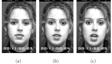
When there are rapid motions in one facial feature (e.g., mouth) due to the changes of facial expressions (see
Figure 4), the corresponding particle filter may fail to track the facial feature’s contour. It is difficult to reduce this failure if we only use multiple independent particle filters to track each facial feature. In this paper, we track several facial fea-tures simultaneously through using several correlated parti-cle filters. When emotion is presented on the face, different facial features have natural physical interaction. For example, when we smile with blinking the left eye, our left mouth tip will move up; when we surprise with the wide-open mouth, the eyebrows will also move up.
Instead of constructing heuristic rules for these rela-tionships, we learn the relationships among facial features from training data beforehand. During the process of track-ing, if we detect that some facial feature tracker’s results are poor, we can infer their positions and states from other
(a) (b) (c)
Figure4: Three consecutive frames at 30 fps show that facial feature
motions are rapid.
facial features by Bayesian inference. In this paper, belief propagation is used to carry out Bayesian learning and inference.
4. COMBINING PARTICLE FILTER WITH BELIEF
PROPAGATION: THE SECOND STEP
4.1. Loopy belief propagation
In every time instant, facial features are contained in an undi-rected graphical modelGf (seeFigure 3). LetV denote the
set of nodes (facial features). Nodes are connected by edges E to describe the relationship between facial features. The neighborhood of a nodeiis NB(i)= {j|(i,j) ∈E}. Letxi
denote the hidden variable (contour of facial feature), and letyidenote the observed variable (facial feature image). Let
{xi} = {xi|1≤i≤N}and{yi} = {yi|1≤i≤N}, whereN
is the number of nodes in the graphical modelGf. The joint
probability density function factorizes as
pxi,yi= 1 C
(i,j)∈E
ψi j
xi,xj
i∈V
φi
xi,yi, (3)
where C is a normalization constant, and ψi j(xi,xj) and
φi(xi,yi) are compatibility functions.ψi j(xi,xj) is a
correla-tion funccorrela-tion betweenxi and its neighbor variablexj, and
φi(xi,yi) is an observation function that denotes the evidence
ofxi[27].
FromFigure 3, we can see that it is a Markov network with loops. Pearl [28] warned that belief propagation might not converge in this kind of graphical models. However, some experimental [29] and theoretical results [30,31,32,
33] motivate us to apply the belief propagation rules in the Markov network with loops, and Murphy et al. called it loopy belief propagation [31].
In belief propagation, we need to calculate the condi-tional marginal distribution p(xi|{yi}) for the nodes that
xi 1 yi 1
xit−1 yi
t−1
M xi t φi yi t ψki ψji
xtj φj ytj xk t ykt φk
. . .
Figure5: Message passing in a directed-cum-undirected graphical
model.
4.2. Belief propagation in spatio-temporal
graphical model
In this paper, the graphical model is the combination of di-rected graph (Markov chain) and undidi-rected graph (Markov network). In order to do Bayesian inference, the key point is belief propagation or message passing.
The messages of directed graph are passing through the time axis. InFigure 5, the message passing fromxti−1toxitis
denoted byM(xi
t−1→xti). We have
Mxti−1−→xit
=pxit|
Yti−1
, (4)
where{Yi
t−1} = {Yti−1|1≤i≤N}, and
pxti|
Yti−1
=
xi t−1
pxit|xti−1
bxti−1
dxit−1. (5)
b(xi
t) is the conditional marginal probability distribution in
nodexi
t, and it is what we have to calculate.b(xit−1) means
the tracking result in facial featureiby graphical model in the previous time instant. The belief at node (i,t) is proportional to the product of the local evidence φi(xit,yit) at that node
and all the messages coming into it [34]. There are two kinds of messages: one comes from the immediate preceding node xit−1temporally, and the other is from the neighbors of node
(i,t) spatially. Therefore, we have
bxi t
=Kφi
xi
t,yit
Mxi
t−1−→xit
j∈NB(i,t)
mji xi t . (6)
In (6),Kis a normalization constant and NB(i,t) denotes the nodes neighboring the node (i,t). As defined in (4) and (5), the message from the previous time is M(xi
t−1 → xti).
Furthermore, the message from the spatial neighbor is de-termined self-consistently by the following message update
rule:
mji
xit
=α
xtj
ψji
xtj,xit
φj
xtj,ytj
Mxtj−1−→xtj
×
k∈NB(j,t)\(i,t)
mk j
xtj
dxtj.
(7)
In the right-hand side of (7), we take the product of mes-sages going into node (j,t) except for the one coming from node (i,t). Note that the message M(xtj−1 → xtj) from the
previous time instant is also taken into account.
Based on a factorization described by [27], we use the observation functionφi(xit,yit)=p(yit|xit), and it can be seen
thatφi(xit,yit) is equal to the observation model in [23]. We
also use the correlation functionψji(xtj,xit)=p(xtj,xit)/ p(xti),
and fit this probability with mixtures of Gaussians [35]. The messageM(xit−1 → xti) passing fromxit−1 toxit can
be viewed as the effective prior: a prediction taken from the marginal probability b(xit−1) from the previous time step,
onto which is superimposed one time step from the dynam-ical model.
From (6) and (7), we can see thatφalways comes with M. By the analysis above, the product of them is
φi
xit,yti
Mxit−1−→xit
=pyi t|xti
pxi
t|
Yi
t−1
= 1 ctp
xi
t|yti,
Yi
t−1
(using (1)).
(8)
Equation (8) means that the product is effectively the poste-rior probability ofxitconditioned onytiand{Yti−1}, and this
shares the same idea with the condensation algorithm. This property is important because it allows us to firstly run the particle filter to track each facial feature in one time step, and the output of particle filter is naturally fitted into a loopy be-lief propagation process (see (6) and (7)).
Wu et al. [36] proposed a mean-field Monte Carlo algo-rithm for visual tracking of articulated human body, which is similar to ours in using the dynamic Markov network.
4.3. Particle propagation in spatio-temporal
graphical model
Since in our spatio-temporal graphical model, messages are not needed to pass backward in the temporal domain, there-fore the choice of importance function can be omitted.
In conventional particle filter algorithms, the probabil-ity distribution of possible interpretations is represented by a randomly sampled set, which can be called “particle set.”
Each sample is a (si
t(m),πti(m)) pair, in whichsit(m) is a
value ofxi
t(m) andπti(m) is a corresponding sampling
prob-ability.m∈[1,M], andMis the total number of samples for one facial feature.
Step1. Firstly, a particularsi
t−1(m) is drawn randomly from
bit−1(m) by choosing it with probabilityπti−1(m) from the set
ofMsamples at timet−1.
Step2. Drawspfit(m) randomly fromp(xi
t|xit−1=sit−1(m)),
one time step of the dynamic model, where pf denotes the particle filter.
Step 3. A value spfit(m) chosen in Step 2 is a fair sam-ple from p(xit|{Yti−1}). Set π pfit(m) = φi(xti = spfit(m),
yti), therefore we obtain the particle set form of φi(xit,
yti)M(xti−1 → xit) ≡ LL(xti), which can be viewed as a
like-lihood function in belief propagation.
Actually,LL(xit) is the tracking result of particle filter for
one facial feature, since we have
LLxti
≡φi
xit,yit
Mxit−1−→xti
= 1 ctp
xit|yti,
Yti−1
(using (8)).
(9)
Using the sampling method similar to conventional parti-cle filter (as described in Steps 1, 2, and 3), we can ob-tain a nonparametric approximation (spfit(m),π pfit(m)) to LL(xti). We can further use a bandwidth selection
method to construct a kernel density estimate LL(xit) from
(spfit(m),π pfit(m)); therefore we can evaluate it in non-parametric belief propagation.
Step 4. Let pmsgji (xtj) denote the foundation of message
mji(xit) as follows:
pmsgji
xtj
≡Kjφj
xtj,ytj
Mxtj−1−→x j t
×
k∈NB(j,t)\(i,t)
mk j
xtj
, (10)
whereKj is a constant which makes pmsgji (x j
t) a probability
density.
Step5. DrawMsamples
s bptj(m)∼Kj
k∈NB(j,t)
mk j
xtj
. (11)
In order to obtain the integral of (7), we should compute a
weight for each sample:
π bptj(m)
∝ p
msg ji
s bptj(m)
k∈NB(j,t)mk j
s bptj(m)
∝φj
xtj,ytj
Mxtj−1−→x j t
|xj
t=s bptj(m)
mi j
s bptj(m)
∝ LL
s bptj(m)
mi j
s bptj(m)
.
(12)
where pmsgji is defined in (10), andmi jis obtained from the
message update in the last iteration.φj(xtj,ytj)M(xtj−1→x j t)
is the result of temporal filter for each facial feature, and we use it to calculate sample weights of messagemji(xit) in (7)
for nonparametric belief propagation.
In (12), althoughLL(xtj) is in particle set form, it still can
be evaluated.
For iterations of message passing, the procedure is initial-ized with all messages set to constant values.
Step6. The approximation of messagemji(xit) is obtained by
mji
xi
t
=M 1
m=1π bp j t(m)
M
m=1
π bptj(m)×ψji
s bptj(m),xti
.
(13)
Step7. Generally, after several iterations of message passing, the belief distribution has converged. We should obtain the marginal estimate forb(xi
t) in (6) to get the final results.
Given the input messagesmji(xit) from the spatial
neigh-bors NB(i,t),
(1) drawMindependent samplessi
t(m),m∈[1,M], from
the product
si
t(m)∼K
j∈NB(i,t)
mji xi t ; (14)
(2) compute the weight for each samplesi t(m):
πi
t(m)∝φi
xi
t,yit
Mxi
t−1−→xti
|xi
t=sit(m)
∝LLsit(m)
. (15)
We also use the result LL(xti) of particle filter in this step
Figure6: Six facial features are described by quadric B-splines.
For samplings bptj(m) inStep 5andsit(m) inStep 7, we
use a similar method to [10]. Sampling from the product can be decomposed into two steps: randomly select one of the product density’s components and then draw a sample from the corresponding Gaussian.
The algorithm in this paper is summarized in the above steps.
4.4. Learning the correlation function
In the training database, we manually mark some face’s fea-tures; therefore we obtain the ground-truth position of the contourxi. First we reduce the dimensionality of facial
fea-turei’s contourxiby PCA. Then from the training data, we
fit mixtures of Gaussians to p(xit) and the joint probabilities
p(xtj,xti) for neighboring facial featureiand j. We evaluate
p(xtj|xit)=p(x j
t,xit)/ p(xit), therefore the correlation function
ψji(xtj,xit) is obtained.
4.5. Optimizing Bayesian inference for
Markov network
Considering that Bayesian inference using belief propagation costs substantial time, we only initiate it when the particle filter’s tracking result is poor.
For the corresponding particle filter on one facial feature, the tracking result on time t can be described by the mo-ments [1]:
Efxt
|Yt
=
M
m=1
πt(m)f
s(tm)
. (16)
As in [1], a mean position using f(xt)= xt can be
uti-lized for graphical display. Moreover, let f(xt) =xtxTt, and
we obtain the varianceσt=E(xtxTt|Yt) of the tracking result.
We use the varianceσtas a metric of the tracking quality.
For each facial feature, we haveσti,i=1,. . .,N, whereN
is the number of all facial features (in this paper, it is 6). For the facial features that have larger variances, we determine that their tracking results are worse than others. Therefore belief propagation is carried out to infer the more plausible positions of their contours. Based on experimental results, if theσi>0.5∗Area(xi), we consider that the tracking result
on facial feature iis bad, where Area(xi) denotes the pixels
occupied by facial featureiin the video stream. In implemen-tation, the Area(xi) is obtained by computing the bounding
box for the facial featurei.
5. EXPERIMENTAL RESULTS
We have developed a prototype system on Windows platform using Visual C++ to implement the algorithm in this pa-per. There are 6 contour models for facial features: eyebrows, eyes, nose, and mouth. Each contour is a quadric B-spline curve, in which contours of nose and eyebrows are open curves, and others are closed curves. As shown inFigure 6, there are 6, 9, 12, 12 control points for left (right) eyebrow, left (right) eye, nose, and mouth, respectively. The total num-ber of control points is 54; therefore the dimensionality is 108.
We choose Cohn-Kanade [37] facial expression database as the training set, because it contains plenty of frontal faces with rich facial expressions. This database is stored as 30 fps grayscale image sequences. To learn the relationships among facial features, we have selected 496 frame frontal face im-ages, which belong to 98 different persons, and used inter-active program to mark each facial feature’s contours. PCA is used to reduce the dimensionality for each facial feature’s contour. After that, the dimensionality of left (right) eye-brow, left (right) eye, nose, and mouth is 4, 7, 9, and 9, respectively; therefore the total dimensionality after dimen-sion reduction is 40, accounting for 99% of the total vari-ance.
After constructing the PCA bases, we compute the cor-responding PCA coefficients for each individual in the train-ing set. For each of facial feature’s contour pairs connected by edges in Figure 3, we determine kernel-based nonpara-metric density estimates for each node itselfp(xit) and their
joint probabilitiesp(xtj,xit).Figure 7shows several
marginal-izations of p(xtj,xit), each of which relates a single pair of
PCA coefficients (e.g., the first mouth and second left eye contour’s coefficients). We can see that simple Gaussian ap-proximations would lose most of this data set’s meaningful structure.
Using the similar method in [23], we have also trained the dynamic model for each facial feature. For observation model, a set of independent measurement lines that are per-pendicular to the hypothesized contour are used to measure the likelihood of detected edge points.
Using a single condensation tracker with multiple con-tours to track multiple facial features is infeasible because the dimensionality is much higher than 10. Here we compare our results with those of multiple independent condensation-style trackers. We have tested our algorithm on the image sequences in Cohn-Kanade database and the videos (640× 480, 30 fps) that we captured by a digital video camera. The test image sequences are not included in the training database.
(a) (b)
(c) (d)
Figure7: Joint density of four different pairs of PCA coefficients. It can be seen that the marginal distributions are multimodal.
(a) (b)
Figure8: Tracking results of a surprise sequence. (a) Our algorithm correctly tracks the eyebrows and mouth. (b) The dark circles and teeth
distract the MICT tracker; therefore it fails to track them.
Figures 8, 9, and 10) show that our tracker is more ro-bust than multiple independent condensation-style trackers (MICT).
In Figure 10, we also compare our algorithm’s results with those of active appearance model (AAM). AAM [15] is based on face alignment, and we use the same training set as MICT to train the active appearance model. FromFigure 10,
(a)
(b)
Figure9: Three consecutive facial expressions: neutral, surprise, and happy. From the first row to second row, and left to right, frame
numbers are 320, 322, 323, 324, 353, 355, 356, 358. (a) Our results. (b) MICT’s results.
incorporate negative samples (e.g., occlusion) into its train-ing set; therefore AAM performs badly when facial feature occlusion happens.
For all the testing image sequences, our algorithm obtains better results than those of MICT and AAM. For the exper-imental results shown in Figures8,9, and10, the image se-quences have 116, 368, and 900 frames, respectively.
Our tracker runs at about 3 Hz, the MICT tracker runs at about 4 Hz, and the AAM tracker runs at about 3.5 Hz on a Pentium 4 1.8 GHz 256 MB RAM computer.
6. CONCLUSIONS
In this paper, we extend the particle filter from the rela-tively simple Markov chain to the directed-cum-undirected graphical model applied to multiple facial feature track-ing problem. Spatial structure information and relationships among nodes in each time instant are effectively considered by Bayesian learning and inference in the loopy belief propa-gation framework.
The advantages of our algorithm are as follows. Com-pared with particle filters, we extend conventional particle filters to track multiple facial features simultaneously by ex-ploring the spatial coherence in each time step, and the com-plexity of tracking is linear rather than exponential in the
number of facial features. Compared with AAM, our algo-rithm is more robust.
The tracking results in this paper can be used as mo-tion capture data. We plan to use these data to derive a 3D face model and generate facial animations. The ultimate pur-pose of multiple facial feature tracking is for facial anima-tion.
Currently, the tracking results are 2D control points of B-splines in each time instant. In the future, we will use these results as video-based motion capture data. Using performance-driven facial animation techniques, we can ob-tain 3D facial animation of the tracked human face from 2D mocap data. Finally we will retarget animation from human faces to other virtual avatars.
(a)
(b)
(c)
Figure10: Comparison results of hiding mouth. Frame numbers
are 802, 803, 805, 810, 871, 872. (a) Our algorithm can success-fully predict the contour of mouth. (b) MICT algorithm failed to track the contour of mouth, which is distracted by the moving hand. (c) AAM algorithm failed too.
ACKNOWLEDGMENT
We would like to thank Dr. Cohn for kindly providing us with the Cohn-Kanade facial expression database.
REFERENCES
[1] M. Isard and A. Blake, “Contour tracking by stochastic prop-agation of conditional density,” inProc. 4th European Con-ference on Computer Vision (ECCV ’96), vol. 1, pp. 343–356, Cambridge, UK, April 1996.
[2] G. Loy, L. Fletcher, N. Apostoloff, and A. Zelinsky, “An adap-tive fusion architecture for target tracking,” inProc. 5th IEEE International Conference on Automatic Face and Gesture Recog-nition (FGR ’02), pp. 248–253, Washington, DC, USA, May 2002.
[3] Y. Rui and Y. Chen, “Better proposal distributions: object tracking using unscented particle filter,” inProc. IEEE Com-puter Society Conference on ComCom-puter Vision and Pattern Recognition (CVPR ’01), vol. 2, pp. 786–793, Kauai Marriott, Hawaii, USA, December 2001.
[4] Z. Zeng and S. Ma, “Head tracking by active particle filtering,” inProc. 5th IEEE International Conference on Automatic Face and Gesture Recognition (FGR ’02), pp. 82–87, Washington, DC, USA, May 2002.
[5] J. Vermaak, P. P´erez, M. Gangnet, and A. Blake, “Towards improved observation models for visual tracking: selective adaptation,” inProc. European Conference on Computer Vision (ECCV ’02), vol. 1, pp. 645–660, Copenhagen, Denmark, May 2002.
[6] P. P`erez, C. Hue, J. Vermaak, and M. Gangnet, “Color-based probabilistic tracking,” inProc. European Conference on Com-puter Vision (ECCV ’02), pp. 661–675, Copenhagen, Den-mark, June 2002.
[7] F. De la Torre, Y. Yacoob, and L. Davis, “A probabilistic frame-work for rigid and non-rigid appearance based tracking and recognition,” inProc. 4th IEEE International Conference on Au-tomatic Face and Gesture Recognition (FGR ’00), pp. 491–498, Grenoble, France, March 2000.
[8] Q. Wang, G. Xu, and H. Ai, “Learning object intrinsic struc-ture for robust visual tracking,” inProc. IEEE International Conference on Automatic Face and Gesture Recognition (FGR ’03), vol. 2, pp. 227–233, Madison, Wis, USA, June 2003. [9] R. van der Merwe, A. Doucet, N. de Freitas, and E. A. Wan,
“The unscented particle filter,” inAdvances in Neural Infor-mation Processing Systems (NIPS), pp. 584–590, Denver, Colo, USA, November 2000.
[10] M. Isard, “Pampas: real-valued graphical models for com-puter vision,” inProc. IEEE Computer Society Conference on Computer Vision and Pattern Recognition (CVPR ’03), vol. 1, pp. 613–620, Madison, Wis, USA, June 2003.
[11] E. B. Sudderth, A. T. Ihler, W. T. Freeman, and A. S. Willsky, “Nonparametric belief propagation,” inProc. IEEE Computer Society Conference on Computer Vision and Pattern Recogni-tion (CVPR ’03), vol. 1, pp. 605–612, Madison, Wis, USA, June 2003.
[12] T. D. I. Essa, S. Basu, T. Darrell, and A. Pentland, “Model-ing, track“Model-ing, and interative animation of faces and heads us-ing input from video,” inProceedings of Computer Animation Conference, pp. 68–79, Geneva, Switzerland, June 1996. [13] Y. Yacoob and L. S. Davis, “Recognizing human facial
expres-sions from long image sequences using optical flow,”IEEE Trans. Pattern Anal. Machine Intell., vol. 18, no. 6, pp. 636– 642, 1996.
[14] M. J. Black and Y. Yacoob, “Tracking and recognizing rigid and non-rigid facial motions using local parametric models of image motion,” inProc. 5th International Conference on Com-puter Vision (ICCV ’95), pp. 374–381, Boston, Mass, USA, June 1995.
[15] T. F. Cootes, G. J. Edwards, and C. J. Taylor, “Active ap-pearance models,”IEEE Trans. Pattern Anal. Machine Intell., vol. 23, no. 6, pp. 681–685, 2001.
[16] J. Ahlberg, “An active model for facial feature tracking,” EURASIP Journal on Applied Signal Processing, vol. 2002, no. 6, pp. 566–571, 2002.
[17] L. Torresani and C. Bregler, “Space-time tracking,” inProc. European Conference on Computer Vision (ECCV ’02), pp. 801–812, Copenhagen, Denmark, May 2002.
[19] Y.-I. Tian, T. Kanade, and J. F. Cohn, “Recognizing action units for facial expression analysis,”IEEE Trans. Pattern Anal. Machine Intell., vol. 23, no. 2, pp. 97–115, 2001.
[20] B. D. Lucas and T. Kanade, “An iterative image registra-tion technique with an applicaregistra-tion in stereo vision,” inProc. 7th International Joint Conference of Artificial Intelligence (IJ-CAI ’81), pp. 674–679, Vancouver, British Columbia, Canada, April 1981.
[21] M. Isard and A. Blake, “ICONDENSATION: unifying low-level and high-low-level tracking in a stochastic framework,” in Proc. European Conference on Computer Vision (ECCV ’98), vol. 1, pp. 893–908, Freiburg, Germany, June 1998.
[22] A. Doucet, N. de Freitas, K. P. Murphy, and S. Russell, “Rao-Blackwellised particle filtering for dynamic bayesian net-works,” inProc. 16th Conference on Uncertainty in Artificial Intelligence (UAI ’00), pp. 176–183, Stanford, Calif, USA, June 2000.
[23] M. Isard and A. Blake, “Condensation—conditional den-sity propagation for visual tracking,”International Journal of Computer Vision, vol. 29, no. 1, pp. 5–28, 1998.
[24] D. A. Forsyth and J. Ponce,Computer Vision: A Modern Ap-proach, Prentice Hall, New York, NY, USA, 2002.
[25] M. Turk and A. Pentland, “Eigenfaces for recognition,”Journal of Cognitive Neuroscience, vol. 3, no. 1, pp. 71–86, 1991. [26] J. B. Tenenbaum, V. de Silva, and J. C. Langford, “A global
ge-ometric framework for nonlinear dimensionality reduction,” Science, vol. 290, no. 5500, pp. 2319–2323, 2000.
[27] S. Geman and D. Geman, “Stochastic relaxation, Gibbs distri-butions, and the Bayesian restoration of images,”IEEE Trans. Pattern Anal. Machine Intell., vol. 6, no. 6, pp. 721–741, 1984. [28] J. Pearl,Probabilistic Reasoning in Intelligent Systems: Networks of Plausible Inference, Morgan Kaufmann, San Mateo, Calif, USA, 1988.
[29] W. T. Freeman, E. C. Pasztor, and O. T. Carmichael, “Lim-its on super-resolution and how to break them,”International Journal of Computer Vision, vol. 40, no. 1, pp. 25–47, 2000. [30] E. C. Liu and J. M. F. Moura, “Fusion in sensor networks:
convergence study,” inProc. IEEE International Conference on Acoustics, Speech, and Signal Processing (ICASSP ’04), vol. 3, pp. 865–868, Montreal, Quebec, Canada, May 2004.
[31] K. P. Murphy, Y. Weiss, and M. I. Jordan, “Loopy belief propa-gation for approximate inference: an empirical study,” inProc. Conference on Uncertainty in Artificial Intelligence (UAI ’99), pp. 467–475, Stockholm, Sweden, July 1999.
[32] Y. Weiss and W. T. Freeman, “Correctness of belief propa-gation in Gaussian graphical models of arbitrary topology,” Neural Computation, vol. 13, no. 10, pp. 2173–2200, 2001. [33] J. Yedidia, W. T. Freeman, and Y. Weiss, “Generalized belief
propagation,” inAdvances in Neural Information Processing Systems (NIPS), pp. 689–695, Denver, Colo, USA, November 2000.
[34] J. S. Yedidia, W. T. Freeman, and Y. Weiss, “Understanding belief propagation and its generalization,” Tech. Rep. TR2001-22, MERL, Cambridge, Mass, USA, 2001.
[35] C. M. Bishop,Neural Networks for Pattern Recognition, Oxford University Press, Oxford, UK, 1995.
[36] Y. Wu, G. Hua, and T. Yu, “Tracking articulated body by dy-namic Markov network,” inProc. 9th IEEE International Con-ference on Computer Vision (ICCV ’03), vol. 2, pp. 1094–1101, Nice, France, October 2003.
[37] T. Kanade, J. F. Cohn, and Y. Tian, “Comprehensive database for facial expression analysis,” inProc. IEEE International Con-ference on Automatic Face and Gesture Recognition (FGR ’00), pp. 46–53, Grenoble, France, March 2000.
Congyong Suwas born in Xinyang, China, in 1979. He received the B.S. and M.S. de-grees from Zhejiang University in 1999 and 2002, respectively, both in electrical engi-neering. Currently he is a Ph.D. candidate in the College of Computer Science, Zhejiang University, and he will graduate in March 2005. His research interests include pattern recognition, computer vision, image/video understanding, and computer facial anima-tion.