78: 6-13 (2016) 95–100 | www.jurnalteknologi.utm.my | eISSN 2180–3722 |
Jurnal
Teknologi
Full Paper
COMPARISON
OF
PRODUCT
QUALITY
ESTIMATION
OF
PROPYLENE
POLYMERIZATION
IN
LOOP
REACTORS
USING
ARTIFICIAL
NEURAL
NETWORK
MODELS
Nur Fazirah Jumari, Khairiyah Mohd-Yusof
*Center for Engineering Education, Universiti Teknologi Malaysia,
81310 UTM Johor Bahru, Johor, Malaysia
Article history Received
13 November 2015
Received in revised form
20 March 2016
Accepted
23 March 2016
*Corresponding author
[email protected]
Graphical abstract
Abstract
One of the major challenges in polymerization industry is the lack of online instruments to measure polymer end-used properties such as xylene soluble, particle size distribution and melt flow index (MFI). As an alternative to the online instruments and conventional laboratory tests, these properties can be estimated using model based-soft sensor. This paper presents models for soft sensors to measure MFI in industrial polypropylene loop reactors using artificial neural network (ANN) model, serial hybrid neural network (HNN) model and stacked neural network (SNN) model. All models were developed and simulated in MATLAB. The simulation results of the MFI based on the ANN, HNN, and SNN models were compared and analyzed. The MFI was divided into three grades, which are A (10-12g/10 min), B (12-14g/10 min) and C (14-16 g/10 min). The HNN model is the best model in predicting all range of MFI with the lowest root mean square error (RMSE) value, 0.010848, followed by ANN model (RMSE=0.019366) and SNN model (RMSE=0.059132). The SNN model is the best model when tested with each grade of the MFI. It has shown lowest RMSE value for each type of MFI (0.012072 for MFI A, 0.017527 for MFI B and 0.015287 for MFI C), compared to HNN model (0.014916 for MFI A, 0.041402 for MFI B and 0.046437 for MFI C) and ANN model (0.015156 for MFI A, 0.076682 for MFI B, and 0.037862 for MFI C).
Keywords: Artificial neural network; soft sensor; propylene polymerization
© 2016 Penerbit UTM Press. All rights reserved
1.0 INTRODUCTION
To improve end-used properties is one of the primary reasons for the use of advanced control in monitoring polymerization reactors. A common problem in the polymer industry is the lack of online instrument for measuring polymer quality [1]. Polypropylene (PP) grade specifications are generally quoted in terms of polymer melt flow index (MFI).
The melt flow index is a widely used indicator of polymer quality [2] which is able to represent the molecular weight distribution of the polymer, where it is the main characteristic of polymer to determine its viscosity, strength and tensile strength. The grade of PP is mainly differentiated by the MFI of the product. The MFI is defined as the mass of polymer in grams flowing
in 10 minutes through a capillary of specific diameter and length, by a pressure applied via prescribed alternative gravimetric weights for alternative prescribed temperatures. Experimental methodology to determine the MFI of polymer resins can be found in [3].
Whenever there is an offset of MFI during the process, it always has a lack of time before the appropriate action is taken because the measure of MFI is done in a period. If the MFI value exceeds from the set point, the product has to be downgraded to cheaper selling or direct disposed due to its inconsistent in MFI in that particular period [5].
Appropriate measures cannot be implemented immediately to bring the process back to normal and minimize the production of off-specification polymer resins. This off-specification product leads to losses and increasing overall production cost. Therefore, early identification of off-specification polymer production is vital.
As an alternative, instead of experimental measurement, polymer MFI can be predicted on-line by developing a soft sensor. A typical soft sensor consists of three main pillars: the process model, the variables used by the model and an update technique. Soft sensor for inferential measurement can be developed using first principle method, multivariate statistical method, or a hybrid of both methods.
The use of neural network has become increasingly popular since the mechanistic models are either unknown or very complex [6-8]. There are many applications of ANN to solve different chemical engineering problems. ANN has been applied by one of the research [9] to develop a detailed mechanistic model of a polyethylene production process including material and energy balance to predict the reactor temperature, conversion and molecular weight distribution (MWD). However the accurate MWD has not been obtained using mechanistic model. Therefore, a feed forward artificial neural network (FANN) has been used to correct the MWDs. In propylene polymerization process itself, the model is developed to predict the end-used property of the final product. A virtual soft sensor to infer MFI of polypropylene has been developed [10] using neural network architecture that integrates independent combining analysis (ICA) and multi-scale analysis (MSA). ICA has been proven effective to estimate the relevance of certain features needed as input to the model. MSA was carried out to acquire more information and to reduce the uncertainty of the studied problem. The proposed method reported can provide prediction reliability and accuracy, which is capable of learning the relationships between process variables and the target MFI. Xia et al. (2010) [11] conducted a study about inferential estimation of polypropylene MFI using stacked neural network based on absolute error criteria. The estimation errors can be reduced by using single neural network model and can be further reduced using stacked neural network model. Gonzaga et al. (2009) [12] focused on measuring viscosity as one of the most important product quality of polyethylene terephthalate (PET). An artificial neural network based on soft sensor (ANN-SS) was developed by using feed forward ANN and trained with the historical dataset of the plant. The proposed ANN-SS was able to provide reliable estimation of the viscosity.
Many researchers have been focusing on the development of the soft sensor using artificial neural network model as mention above. Nevertheless, the comparison of effectiveness on of various types of ANN models is limited in literatures. Therefore in this paper artificial neural network (ANN), serial hybrid neural network (HNN) and stacked neural network (SNN) models were developed to predict the MFI of polypropylene in industrial loop reactors. Using these models, the MFI can be estimated from the measured process variables instantly.
2.0 PROCESS DESCRIPTION
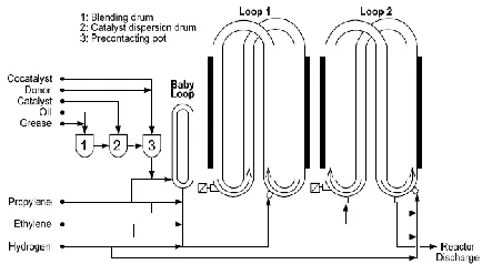
Understanding the process helps in determining the variables and parameters involved to develop ANN models. Therefore, this section will elaborate about the process of propylene polymerization in industrial loop reactors. Figure 1 shows the industrial loop reactors modeled in this study. This figure illustrates the typical set up for loop reactor used for propylene polymerization plant in Malaysia.
Loop reactors are widely used in large-scale coordination polymerization industries because they offer low capital and maintenance cost, high production rate, high heat removal, and maintain uniform temperature, pressure and catalyst distribution. The reaction is a liquid phase propylene polymerization which is a part of the Spheripol process. The Spheripol process comprises of three steps, namely catalyst and raw material feeding, polymerization and finishing. The fourth-generation of Ziegler Natta catalyst is used due to its high activity and stereospecificity [13].
Figure 1 Process flow diagram of industrial loop reactor
3.0 MODELS DEVELOPMENT
3.1 Data Collection
The very first step to develop the ANN, HNN and SNN models was to gain information on the selected input data and requirements to build the network architecture. The input variables were selected depending on the factor of dynamic behavior of the chemical process, and kinetic reaction of the polymerization.
The kinetic mechanism of the propylene polymerization reaction involved the catalyst, cocatalyst, donor, hydrogen and monomer affected the PP reaction. The propylene was the main substance in this polymerization process. The flow rate of catalyst, co catalyst and donor were chosen to show the generation of the active site of catalyst. The active catalyst site reacted with the monomer, hydrogen and cocatalyst, Triethylaluminium (TEAL) to form PP with certain chain length during transfer reaction step. Time was considered as input of the model to show the dynamic behaviour of PP because the polymerization process was changed with time as nonlinear process.
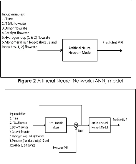
The output variable in this study is the MFI of the polymer. The MFI was divided into three grades which are MFI A (10-12 g/10 min), MFI B (12-14 g/10 min) and MFI C (14-16 g/10 min). These grades are categorized according to the given range in order to analyze them thoroughly. Figure 2 shows the input and output variables for ANN model. For HNN model, the error between actual MFI and MFI generated first principle model [14-17] was added as an additional input as shown in Figure 3.
Figure 2 Artificial Neural Network (ANN) model
Figure 3 Serial Hybrid Neural Network (HNN) model
3.2 Development, Simulation And Validation Of
ANN Models
The built up of feed forward back propagation (FFBP) neural network can be divided into two major steps, which are network training and network testing. Then, the model was validated using the cross validation (unseen) data for all combined MFI. The data distribution to develop the models is shown in Table 1. The function ‘newff’ in MATLAB created a feed-forward model and requires three basic arguments, which are input vector, target vector and array containing the size of each hidden layer. Another argument is a cell array containing the name of the training function. The transfer function used in the hidden layer is tansig and pureline for the output layer. Levenberg-Marquadt was chosen as the training algorithm due to the fast back-propagation algorithm in the toolbox and highly recommended as a first choice algorithm. Once a neural network is created, it needs to be configured and trained. Then, the network underwent the testing generalization. The investigation of ANN model was continued by pruning the unnecessary inputs networks. For each network structure that being developed, the initial weights and biases which showing smallest RMSE were recorded.
3.3 Development, Simulation And Validation Of
HNN Model
The hybrid neural network uses the residue of MFI extracted from the first principle model [14-17] and actual data as an additional input into the ANN model. The first principal part consists of a set of nonlinear differential equations, resulting from relevant mass and population balance [16-17].
The MFI model was developed according to power-law-type correlation, as a function of polymer weight average molecular weight (WAMW). The correlation was developed based on polymer WAMW values from first principles simulation results and MFI values from experimental measurement from industry.
As the MFI model is developed in the form of a power-law-type correlation, it is valid in a limited range of WAMW. Each MFI spec will require different MFI model. The developed MFI model is validated using other sets of industrial data in order to examine its accuracy and reproducibility. The example of relationship between MFI and polymer WAMW as a power-law-type model is illustrated in Figure 4.
Figure 4 MFI-WAMW relationships as a power-law-type
model
Table 1 Data distribution for ANN and HNN model
Data distribution
Types of MFI
A (10-12 g/10min)
B (12-14 g/10 min)
C (14-16 g/10min) Training data set 34 30 32
Testing data set 11 8 8
Validation 5 5 5
3.4 Development, Simulation And Validation Of
SNN Model
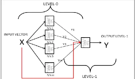
Stacked neural network (SNN) was proposed to improve the accuracy of the model due to a limited number of training data sets. Model accuracy was improved by combining several neural networks [18]. Wolpert (1992) concluded that stacked generalization can be expected to reduce the generalization error rate. Two layers were needed in constructing stacked neural network: level-0 and level-1. Level-0 generalizer output came from a number of diverse ANN models, each of which was trained and tested on independent data set. The level-1 generalizer was developed by using the results of level-0 generalizer. Level-1 generalizer was trained by using the prediction of the level-0 models and the target value of level-0 validation data set.
In this paper, the developed ANN and HNN models above were combined in a stacked neural network. The data distribution to develop SNN model are shown in Table 2.
Table 2 Data distributions for stacked neural network model
Data distribution
Types of MFI
Total
A (10-12 g/10min)
B (12-14 g/10 min)
C (14-16 g/10min) Training and
testing (level-0) 45 38 40 115 Overall Testing
(level-1) 5 5 5 15
The technique to produce level-1 data set for the stacked neural network was based on a simple example by Sridhar, Seagrave and Bartlett [19]:
1. Set the level-0 data set DL0 equal to data set D. Train the M level-0 network using DL0. Denote the jth network trained on DL0 as Nj(DL0), and denote the set of these level-0 network as N(DL0)={Nj(DL0):1≤ j≤M}. The N(DL0) should be saved for use in the SNN model.
2. Each type of MFI’s data is divided into three equal parts. Suppose DL0 is the overall data, D is divided into D1, D2 and D3. Define CVi as D-Di. CVi contains all the pattern in the data set D except the pattern in Di. For example, CV1 is D-D1.
3. Train the M candidate ANN models using the data set CVi. Denote the jth network trained on CVi as Nj(CVi), and denote the set of these trained network as N(CVi)={Nj(CVi):1≤ j ≤M}. The reason for developing the networks N(CVi) is to construct level-1 data set DL1. Recall N(CVi) on the data set Di. Denote the prediction of the jth network for pattern n in the data set Di as ypnj. For pattern n, the output of the candidate models is collected in an M-dimensional vector ypn={ypnj:1≤ j ≤M}. The actual output yn and the network output ypn constitue the output and input respectively, for the nth pattern in data set DL1. Discard the networks {Nj(CVi):1≤ j ≤M}. 4. Step 3 produces the level-1 data set DL1(yn,
ypn). Data set DL1 contains the true output and the predictions of the M models, for all N training patterns.
The steps above generated 18 data sets consist of all types of MFI for ANN and HNN model. As an example, for MFI A, three data set produced from ANN model and another three from HNN model. MFI B and MFI C also produced three data set from ANN model and HNN model. The single networks for MFI A, B and C were developed by varying the amount of hidden nodes and weights. Each respective single network model was trained for ten times from 5 to 30 different numbers of hidden nodes. The validation error (RMSE) for each single network with their respective weights and biases for particular hidden nodes were identified. The selection of the best single networks according to its weights and biases was based on the best validation result.
Figure 5 Stacked Neural Networks (SNN) Model
4.0 RESULT AND DISCUSSION
The neural network models (ANN, HNN and SNN) developed will be tested with the different data distribution: all ranges of MFI and each grades of the MFI. This is because, certain models are only able to give the better prediction result for certain MFI.
Table 3 shows the results for the neural network models when use the summation of all grades of MFI. As shown in Table 3, all the models generated the RMSE below 6% . HNN model is the best model to predict overall MFI types with the least RMSE, 0.010848. This is because its capability to calculate the residue between actual plant data MFI value and simulated MFI. The ANN model gives 0.019366 RMSE values. The number of nodes required are 27. In order to secure the ability of the network to generalize, the number of nodes has to be kept as low as possible. Having a large excess of nodes, the network will become like a memory bank that can recall the training set to perfection, but it did not perform well on samples that was not part of the training set. The stacked neural network (level-1) gave the highest RMSE (0.059132) as compared to the ANN and HNN model when predicting the overall MFI types.
Table 3 The performance of the neural network model
Types of Model No of
hidden nodes
R2 RMSE
ANN Model 27 0.977895 0.019366 HNN Model 20 0.994395 0.010848
SNNModel
(level-1) 5 0.851910 0.059132
For further investigation, the ANN, HNN and SNN models were tested with each type of MFI. Table 4 shows the performance of the models for each MFI. As compared to others model, the stacked neural network model has shown the lowest RMSE for each type of MFI. The capability of the stacked neural network to effectively integrate the knowledge acquired by different networks can produce better prediction. Stacked neural network had shown good results for the experiments with different grades of MFIs. In addition,
the stacked neural network set up with different types of network such as hybrid, and normal neural networks provide accurate expectations. So stacked neural network has been providing the most optimal ways to anticipate the target values.
Table 4 The performance of the models to predict each grades
of MFI
Types of Model ANN Model HNN Model SNN Model
(level-1)
No of nodes in
hidden layer 20 27 6
Types of MFI RMSE RMSE RMSE A
(1012g/10min) 0.015156 0.014916 0.012072 B
(12-14g/10min) 0.076682 0.041402 0.017527 C
(14-16g/10min) 0.037862 0.046437 0.015287
5.0 CONCLUSION
In this work, the single artificial neural network (ANN), hybrid neural network (HNN) and stacked neural network (SNN) models were successfully developed to predict melt flow index (MFI) for the Spheripol propylene polymerization process. The models developed were tested with all ranges of MFI and each grade of MFI data.
From the finding, the single HNN model is the best model to predict all ranges of MFI with RMSE value is 0.010848, followed by ANN (RMSE=0.019366) and SNN models (RMSE=0.059132). It is because the first principle models described certain characteristics of the process being simulated. The introduction of the additional information (residue of MFI extracted from the first principle model) generated from the first principle model assisted the HNN model to perform better in predicting the MFI.
The SNN model (with the number of nodes in level-1 is 6) is the best model once tested with each type of MFI. It gave the lowest RMSE value for each type of MFI (0.012072 for MFI A, 0.017527 for MFI B and 0.015287 for MFI C). The capability of the SNN to effectively integrate the knowledge acquired by different networks can produce better prediction. The stacked neural network is a general method of using the high level model to combine lower level model to achieve greater predictive accuracy. It was set up with different types of network and the input variables provided accurate expectations. The SNN is also recommended when only a limited number of data is available
Acknowledgement
We are grateful for the UTM Zamalah scholarship for Author 1 and eSCIENCE fund Project Number R.J130000.79094S130.
References
[1] Kim, M., Lee, Y.H., Han, I.S., and Han, C. 2005. Clustering Based Hybrid Soft Sensor for an Industrial Polypropylene Process with Grade Changeover Operation. Ind. Eng. Chem.
Res. 44: 334-342.
[2] Peacock, A. J. 2000. Handbook of Polyethylene: Structures, Properties, and Applications. New York: Marcel Dekker. [3] Latado, A., Embirucu, M., Neto, A. G., & Pinto, J. C. 2001.
Polymer Modelling: Modelling of End Use Properties of Poly (propylene/ethylene) Resins. Polymer Testing. 20: 419-439. [4] Zhang, J.,Qi, B.X., and Yong, M. 2006. Inferential Estimation of
Polymer Melt Index Using Sequentially Trained Aggregated Neural Network. Chem. Eng. Technol. 44: 442-448.
[5] Ghasem, N.M., Sata, S.A., and Hussain, M.A. . 2007. Temperature Control of a Bench-Scale Batch Polymerization Reactor for Polystyrene Production. Chem. Eng. Technol. 30(9): 1193–1202.
[6] Fernandes, F. A. N. and Lona, L. M. F. 2005. Neural Network Applications in Polymerization Processes. Braz. J. Chem. Eng. 22(3): 401-418.
[7] Azaman, F., Azid, A., Juahir, H., Mohamed, M., Yunus, K., Toriman, M. E., & Hairoma, N. 2015. Application of Artificial Neural Network and Response Surface Methodology for Modelling of Hydrogen Production Using Nickel Loaded Zeolite. Jurnal Teknologi. 77(1): 109-118.
[8] Dashtbayazi, M. R., & Ghanbarian, M. 2015. Comparison of Artificial Neural Network Methods in Modeling of Polymer Matrix Composite Turning. Mechanical Engineering. 47(2). [9] Hinchliffe, M., Montague, G., and Willis, M. 2003. Hybrid
Approach to Modeling an Industrial Polyethylene Process.
AIChE Journal. 49(12): 3127-3137.
[10] Jian S., Xinggao L., and Youxian S. 2006. Melt Index Prediction by Neural Network Based in Independent Component Analysis and Multi-Scale Analysis. Neurocomputing. 70(2006): 280-287.
[11] Xia, L., and Pan, H. 2010. Inferential Estimation of Polypropylene Melt Index Using Stacked Neural Network Based on Absolute Error Criteria. International Conference on Computer, Mechatronics, Control and Electronic Engineering. (2010): 216-218.
[12] Gonzaga, J.C.B., Meleiro, L.A.C., Kiang, C., and Maciel Filho, R. 2009. ANN-based Soft-Sensor for Real-Time Process Monitoring and Control of An Industrial Polymerization Process. Computer and Chemical Engineering. 33(2009): 43-49.
[13] Albizzati, E., Giannini, U., Collina, G., Noristi, L., and Resconi, L. 1996. Catalyst and Polymerizations. In Moore, E. P. (Ed.) Polypropylene Handbook. New York: Hanser Publisher. (): 11-111.
[14] Zacca, J. J. and Ray, W. H. 1993. Modelling of The Liquid Phase Polymerization of Olefins in Loop Reactors. Chemical
Engineering Science. 48(22): 3743-3765.
[15] Lucca, E. A., Filho, R. M., Melo, P. A., and Pinto, J. C. 2008. Modeling and Simulation of Liquid Phase Propylene Polymerizations in Industrial Loop Reactors. Macromolecular
Symposia. 271: 8-14.
[16] Harun, N. F. 2009. Formulation of Modeling and Simulation Algorithm for Propylene Homopolymerization in Industrial Loop Reactors. M. Eng. Project Report, Skudai. Malaysia: Universiti Teknologi Malaysia.
[17] Jamaludin, M. Z. 2009. Modelling The Product Quality and Production Rate Of Propylene Polymerization In Industrial Loop Reactors. M.Eng. dissertation, Malaysia: Universiti Teknologi Malaysia.
[18] Wolpert, D.H. 1992. Stacked Generalization. Neural Networks. 5: 241-259.