Multiple trait analysis of genetic mapping for quantitative trait loci.

Copyright 0 1995 by the Genetics Society of America

Multiple

Trait

Analysis

of

Genetic Mapping

for

Quantitative

Trait

Loci

Changjian

Jiang* and

Zhao-Bang Zengt

*Department of Agronomy, Jiangsu Agricultural College, Yangzhou, Jiangsu 225001, People's Republic of China and Program in Statistical Genetics, Department of Statistics, North Carolina State University, Raleigh, North Carolina 27695-8203

Manuscript received September 22, 1994

Accepted for publication March 30, 1995

ABSTRACT

We present in this paper models and statistical methods for performing multiple trait analysis on

mapping quantitative trait loci (QTL) based on the composite interval mapping method. By taking into

account the correlated structure of multiple traits, this joint analysis has several advantages, compared

with separate analyses, for mapping QTL, including the expected improvement on the statistical power

of the test for QTL and on the precision of parameter estimation. Also this joint analysis provides formal

procedures to test a number of biologically interesting hypotheses concerning the nature of genetic

correlations between different traits. Among the testing procedures considered are those for joint

mapping, pleiotropy, QTL by environment interaction, and pleiotropy vs. close linkage. The test of

pleiotropy (one pleiotropic QTL at a genome position) vs. close linkage (multiple nearby nonpleiotropic

QTL) can have important implications for our understanding of the nature of genetic correlations

between different traits in certain regions of a genome and also for practical applications in animal and

plant breeding because one of the major goals in breeding is to break unfavorable linkage. Results of

extensive simulation studies are presented to illustrate various properties of the analyses.

M

ANY

data for mapping quantitative trait loci

(QTL) contain observations on multiple traits

or on one or several traits in multiple environments.

With such data, we can ask questions like the following:

Does a QTL have pleiotropic effects on multiple traits? Does a QTL show genotypeenvironment interaction?

What is the nature of genetic correlation between differ-

ent traits? Is the correlation due to pleiotropy or linkage

in certain regions of a genome? Statistically this involves

multiple trait analysis, because the expression of a trait in different environments can be regarded as different

traits or different trait states (FALCONER 1952).

Currently, the many statistical methods developed for

mapping QTL ( e.g., LANDER and BOTSTEIN 1989; HALEY

and KNOTT 1992; JANSEN and STAM 1994; ZENG 1994) are for analysis on one trait only and have not been

extended specifically for multiple trait analysis yet. With

that omission, a number of studies on mapping QTL (e.g., PATERSON et al. 1988, 1991; STUBER et al. 1992) analyzed different traits separately. This approach does not take advantage of the correlated structure of data and has a number of disadvantages for mapping QTL

and also for understanding the nature of genetic corre-

lations. The statistical powers of hypothesis tests tend to be lower and the sampling variances of parameter

estimation tend to be higher for separate analyses. Also,

it would be difficult to test a number of biologically interesting questions involving multiple traits by analyz- ing different traits separately.

North Carolina State University, Raleigh, NC 276958203. E-mail: [email protected]

Corresponding authur: Zhao-Bang Zeng, Department of Statistics,

Different traits are correlated genetically due to plei- otropy and linkage. With observations on a number of polymorphic genetic markers and on a number of quantitative traits, it is possible to dissect a portion of genetic variation and covariation among traits by lo- calizing and estimating responsible QTL. It is also possi-

ble to test whether the genetic correlation is due to

pleiotropy or linkage for certain regions of a genome. In this paper, we extend the composite interval map-

ping method ( ZENG 1993, 1994) to multiple trait analy-

sis. We demonstrate how the joint analysis on multiple traits can improve the power and precision of mapping QTL; we show how to test some biologically interesting hypotheses involving multiple traits, such as pleiotropy

and QTL X environment interaction, and how to test

whether significant associations for different traits in

certain regions of a genome are due to pleiotropy or

close linkage. Properties and behavior of the test statis- tics are examined by analyses and also by simulation studies.

STATISTICAL MODELS AND LIKELIHOOD ANALYSES

Composite interval mapping model for multiple traits:

In this section, we formulate statistical models and

likelihood analyses for mapping QTL that affect mul-

tiple traits, using the composite interval mapping

method.

Suppose that we have a sample of n individuals

from an F2 population crossed from two inbred lines,

with observations on m quantitative traits and on a

number of codominant genetic markers. Let the

1112 C. Jiang and Z.-B. Zeng

TABLE 1 b, and d , are partial regression coefficients of Y ] k on

Probability of QTL genotype given xjl and zjl; and ejk is the residual effect on trait k for

It is assumed that the residual effects e,bs (the error

flanking marker genotype individual j .

QTL genotype

Marker

genotype (2)

44

( 1 ) 44 ( 0 )

p

= ~ M , Q / ~ M ~ M ~ , 6 = r & ~ ~ / [ ( l - rMlM2)’

+

r&M2], where

rhflQ is the recombination frequency between marker MI and

QTL and rMIM2 is the recombination frequency between

markers MI and M2. Double recombination is ignored.

value of each marker be recorded as

2,

1 and 0 for

the homozygote in one parental line, heterozygote

and homozygote in the other parental line, respec-

tively. These markers can be mapped in linkage

groups or mapped on chromosomes if the locations

of some of them are known.

Further, let y j k denote the value of the kth trait in the

j t h individual. To test for a QTL on a marker interval ( i,

i

+

1 ) , the statistical model for mapping QTL for one

trait ( ZENC 1994) can be readily extended for mapping

QTL for multiple traits as follows:

y j l = bo,

+

bT.7

+

drzT

+

( & I xjl

+

dllzjl)

+

ql

,

1

1 1

, I ] Z = bo2

+

b,*

x7

+

d : ~ ?

+

C

(biz xjl

+

dl29l)

+

ejn,

1

I

y ] m = born

+

bEx7

+

dEz7

+

( b l m x j l

+

&rnzil)

+ q m ,

1

j = 1,

. . . ,

n, ( 1 )

where ylk is the phenotypic value for trait k in individ-

ual j ; bok is the mean effect of the model for trait k ;

b f is the additive effect of the putative QTL on trait

k ;

XT

counts the number of the allele at the putative QTL from one of the two parental lines, say parent

Pl [taking values of 2, 1 and 0 with probabilities de-

pending on genotypes of the markers i and i

+

l

flanking the putative QTL and the recombination fre- quencies between the QTL and the markers (Table

1 ) ] ; d f is the dominance effect of the putative QTL

on trait k ; z? is an indicator variable of the heterozy-

gosity at the QTL taking values 1 and 0 for heterozy-

gote and homozygotes (Table 1 ) ; xjl and zll are corre-

sponding variables for marker

I,

assuming t markers

are selected for controlling residual genetic variation;

terms) are correlated among traits within individuals

with covariance Cov(

q k ,

e i l ) = = pklakgl but are

independent among individuals. For likelihood analy-

sis, it will be further assumed that

qg

are multivariate

normally distributed among individuals with means

zero and covariance matrix

J. .

In matrix notation, model ( 1 ) can be expressed as

Y = x* b*

+

z * d*

+

X B

+

E ,

( 3 ) n X m nX1 I X r n n x l I X m n x ( 2 1 + 1 ) ( 2 t + l ) x m n x m

where Y is a ( n X m ) matrix of y j k ; x * is a ( n X 1 )

column vector of x;” ; z

*

is a ( n x 1 ) column vector

of z;”; b* is a ( 1 X m ) row vector of b f ; d* is a ( 1 X m ) rowvectorof d f ; X i s a

[ n x

( 2 t +

l ) ]

matrixof

data on t markers, xjls and zjls, fitted in the model as

background control, including also the mean effect; B

is a [ ( 2 t

+

1 ) X m ] matrix of b,, d,, and

4 k ;

and E is a ( n X m ) matrix of elk.

The reasons to include multiple markers in the re- gression model for testing and estimating the putative

QTL effects are mainly twofold. First, these markers can

control and eliminate much of the background genetic variation from the residual variances and covariances of the model and thus can increase the statistical power for mapping QTL. Second, if some linked markers are also fitted in the model as background control, these markers can block the effects of other possibly linked

QTL in the test and thus can reduce the chance of

interference of possibly multiple linked QTL on hy- pothesis testing and parameter estimation. These prop-

erties of multiple regression analysis have been dis-

cussed in detail by ZENG (1993, 1994) in reference to

QTL mapping for one trait and can be directly applied to QTL mapping on multiple traits.

In model ( 1 )

,

for simplicity it is assumed that t

markers are each fitted with additive and dominance

effects for genetic background control. Since many

different markers can be fitted in the model, the ques-

tion of selecting how many and what markers to be fitted in the model becomes a major issue for map-

ping QTL. A number of considerations have to be

taken into account for such a selection process, and many relevant issues involved have been discussed in

ZENC (1994). Here, we concentrate our discussion on the extension of the method to multiple trait anal- ysis and avoid lengthy discussion on this issue.

Mapping QTL on Multiple Traits 1113

variate normal distribution of error terms, the likeli-

hood function of the data is defined as

n

~1

n

[bjft

(yj)

+

hjJ

( y j )

+

pOjfO(yj)

I

> ( 4 )

j = l

where

p j ,

plj

and

poj

denote the prior probability of

x? taking values 2, 1 and 0 , respectively, for the three

genotypes of the putative QTL (Table 1 ) , and

f2

(

y j )

,

fi

(yj)

and

fo

(yj)

represent the multivariate normal

density functions of the vector variable

y j

(the jth row

of Y ) with means uj2 = x,B

+

2b*, ujl = xjB

+

b*

+

d*, and ujo = x,B, respectively, and the covariance matrix (

2 )

.

Then, by applying standard maximum likelihood pro-

cedures, the maximum likelihood estimates of parameters

can be found as in the following. As in ZENG (1994),

these maximum likelihood estimates can be computed by

iteration through an ECM algorithm (MENG and RUBIN

1993) that is a special version of general EM algorithms.

In the ( v

+

1 ) th iteration, the &step ( k . , expectation

step) calculates the posterior probabilities of individual j

being a particular genotype at the putative QTL as

q $ J + l ) =

bjf6")

( y j )

/

[&jf6") ( y j )

qi;+l) = P1jf

1")

(yj)

/

[hjfi")

(yj)

& + I ) =

Ajf6")

( y j )

/

[ b j f 6 " '

(yj)

+

p1jf

I"'

(yj)

+

Ajf6"'

(yj)

I ,

+

pljff")

(yj) +

hjf6")

(yj)

I9

+

hjf

1") (yj)

+

p o ~ f 6 " '

(yj)

I

> ( 5 )

where f

6")

(

y j )

,

f

1'

") (

y j )

and

f

6")

( yj) are the corre-

sponding normal density functions with parameters re-

placed by estimates in the

vth

iteration. In the CM-step

(i.e., conditional maximization step), parameters in

f2

(yj)

,

fi

(E)

and

fo

(yj)

are divided into three groups,

(b*, d * )

,

B ,

V,

and estimated consecutively between

groups but simultaneously within each group. These estimators can be shown to be as follows:

b*("+l) = q p l ) ' ( Y - X B ( u ' ) / ( 2 q ~ " + 1 " 1 ) , ( 6 )

d*("+1) = ( u + l ) f / ( q $ U + l ) f l ) [ S I

- q$"+l)'/ (2q$"+"'l) ] (Y

-

XB'")),

( 7 )

B ( " + ' ) = (X'X)"X'[y - (2q4"'1)

+ q(lu+l))b*(v+l) - (V+l)d*(U+')

91

I ,

( 8 )

v ( u + l ) = [ ( y - = ( " + I ) ) ' ( y - = ( " + I )

)

- 4(qhU+1)rl)b*(u+l)'b*(U+1)

- ( q $ u + l ) f l ) (b*(U+l) + d*(U+l)

x

( b * ( u + l ) + d*(V+1)

) '

) I / %

( 9 )

where q p ' ) and q$"+l) are ( n

x

1) vectors of q$'+')

and qiy"), and 1 is a column vector of ones. A prime represents the transpose of a matrix or a vector.

The calculation begins with q$') =

&,,

q$:) =

plj,

& ) =

hj,

and some starting values for b* ( O ) and d* ( O )

(one possible choice is to set them to zero)

.

Iterations

are then made between ( 5 ) , ( 6 ) , ( 7 ) , ( 8 ) , and ( 9 ) and terminated when a predetermined criterion is satis- fied. The criterion for termination is set to be that the changes of the parameter estimates, or the increment of the log-likelihood value, at each iteration become

less than E ( a small positive number, say,

lo-').

The

final estimates are denoted as b*, d*, B and

e,

which

will then be used for the calculation of the maximum likelihood value for hypothesis testing.

The log-likelihood of ( 4 ) is calculated, with the pa-

rameters replaced by the estimates, as

ln(L1) = K - ( n / 2 ) ln(1VI)

n

+

C.

M & , e x p [ - ( 1 / 2 )

x

(yj -

21;"

- X j B ) V "

x

(y3

-

b *

-

d *

- XjB)V"

x

(yj

-

b *

-

d *

- XjB)

'1

X ( y j - x$)'II

3=1

X

(yj-

21;* -

xjB)'I

+ p l j e x p [ - ( 1 / 2 )

+ p o , e x p [ - ( 1 / 2 ) ( y , - ~ ~ B ) V - ~

= K - ( n / 2 ) ln(lV1) - ( 1 / 2 )

n

x

(yj - xjB)V-l (yj - XjB)'

j = l

n

+

ln{p2,exp[21;*V"(y.- I

b*

- xjB)']

+

plj

exp[

(b*

+

d*)V"

(yj - b*/2

j = l

- d * / 2 - XjB)'1

+

P o , ) ,

(10)

where

191

is the determinant of the covariance matrix,

and K = -nm ln(27r)/2.

Numerical procedures of the ECM algorithm. Here

we explain how the ECM algorithm involving ( 5 )

-

( 9 )

can be implemented efficiently. Computationally, the

major element of the analysis involves least squares anal-

ysis or, more specifically, the calculation ofY - XI$("+')

in each step. Numerically, least squares analysis is usu-

ally performed through a QR factorization of matrix X.

Namely, for an ( n X m ) X matrix (assuming n

>

m )

,

we can decompose X as

X = (QI Q P )

(t)

= QIR, (11)

where Q = (Q1, Q2) is an ( n X n) orthogonal matrix

(i.e., Q'Q = I ) and is partitioned into two parts, Q1

1114 C. Jiang and Z.-B. Zeng

usual least squares estimates B and Y - XB (residuals)

can be calculated as

B = (X'X)"X'Y = (R'QiQ,R)"R'Q;Y

= R - ~ Q I Y , ( 1 2 )

Y - XB = Y - Q,RR-'Q;Y = ( I - Q I Q ; ) Y . (13)

In our numerical implementation, before entering

the ECM loop, X is first factorized into Q and R by

Householder transformations using the LINPACK rou-

tines ( DONGARRA et al. 1979). In each loop, Y - XB is

obtained by first calculating

W = [Y - (2qz

+

q l ) b * - q1d*] - XB = Y - XB

= ( I

-

Q ~ Q ; ) ~ ?

(14)

from (13) and then recovering from W

Y -XB = W

+

(2q2

+

q l ) b *

+

qld*. (15)

This is used for calculation in ( 5 ) , ( 6 ) , ( 7 ) , and ( 9 ) .

Equation 8 becomes redundant and is omitted in calcu-

lation. These numerical procedures are the same proce-

dures used by ZENG ( 1994).

Since X is unchanged in each loop,

Q

is unchanged.

The above calculations become very simple updates in each loop. This illustrates the numerical advantage of the ECM algorithm, compared with the full EM algo-

rithm ( e.g.,JANSEN 1992) that groups x* and z * (repre-

sented by qs) into X and factorizes or updates factoriza-

tion of X in each loop to obtain B (which includes b

*

and d* ) and V. The convergence of the ECM algorithm

to maximum likelihood estimates has been proven by MENC and RUBIN ( 1993).

HYPOTHESIS TESTS OF QTL EFFECTS

In hypothesis testing, model ( 1 ) is usually called the

full model. With some parameter values constrained to some specific values, a number of null hypotheses can be constructed and tested. For mapping QTL, we are mostly concerned with testing hypotheses about the ad- ditive and dominance effects of QTL. However, before we test other hypotheses, we need first to test for the presence of QTL. Without losing generality, we restrict

our discussion to two traits.

Joint mapping €or QTL on two traits: With pheno-

typic observations on two traits, mapping for QTL can

be performed for each trait individually or jointly on both traits. Under the joint mapping, the hypotheses to be tested are

*

*

H,: bl = 0, dl = 0, b,* = 0, d,* = 0,

HI : At least one of them is not zero. (16)

The log-likelihood under Ho is then

l n ( b ) = ln n J ( y j ) [ j : l

1

= K - ( n / 2 ) In(

I V , / )

- nm/2, (17)

where V o = ( Y - X&,)'(Y - X & , ) / n and

8,

=

( X ' X ) "X'Y. The test is performed with a likelihood ratio statistic

LRl = -2 l n ( & / L l ) . (18)

Under H,, the likelihood ratio LRl will be approxi-

mately chi-square distributed. The determination of the critical value for the test is, however, very complicated. The complication is largely due to the fact that the test is usually performed for the whole genome, a situation of multiple tests. With multiple tests, the critical level for each test has to be adjusted. It has been shown

( ZENG 1994) that, for the composite interval mapping, tests in different intervals are close to being indepen- dent except for those in adjacent intervals that are

slightly correlated. Thus, if we choose a' as the genome-

wise error rate, the error rate of the test per interval,

a ,

can be approximated by using the Bonferroni correc-

tion as a = 1 - ( 1 - a ' ) I", or to a good approxima-

tion as

a

= a ' / M , where M is the number of intervals

involved in the test. The maximum of the test statistic within an interval can be roughly approximated by a

chi-square distribution with a degree of freedom 2m

+

1 (the number of parameters under the test including

one for the position of the putative QTL) [see the

simulation study of ZENC ( 1994) for m = 1 and a back-

cross design]. Thus, in practice, we may use

x

~

/

to approximate the critical value of the test

~

~

~

~

+

~

in this situation (for two traits m = 2 )

.

However, we

emphasize that the correct determination of appro-

priate critical value for this test is a very complicated

statistical issue. The above recommendation is sug-

gested only for a very rough approximation. Recently, CHURCHILL and DOERGE ( 1994) proposed to use a per- mutation test to empirically estimate the genome-wise critical value for a given data set and a given test. Their method can be extended for multiple trait analysis.

Why do we need to perform joint mapping? First, the

joint analysis on two traits can provide formal proce-

dures for testing a number of biologically interesting hypotheses, such as pleiotropic effects of QTL, QTL by

environment interaction and pleiotropy us. close link-

age, as shown below. Second, if the putative QTL has pleiotropic effects on both traits, the joint mapping on both traits may perform better than mapping on each trait separately.

In APPENDIX A , the relative advantages of the joint analysis as compared to separate analyses are discussed. It is shown that the test statistic for the joint analysis

is always higher than that for each separate analysis.

However, this does not necessarily mean that the power

of the test will be increased by using more traits, because more parameters will be included in the model for test-

Mapping QTL on Multiple Traits 1115

ing. When the residual correlation p = 0 , the test statis-

tic under the joint test is approximately the sum of those under separate tests. Otherwise the joint test sta- tistic can be smaller or larger than the sum of separate test statistics, depending on the sign and magnitude of the residual correlation and the differences between QTL effects. The power of the joint test can increase significantly if the relevant QTL has pleiotropic effects

on two traits with the product of the effects in different

direction to the residual correlation. If the product of pleiotropic effects and the residual correlation are in the same direction, however, the test statistic under the

joint test will be smaller than the sum of the test statistics

under the separate tests. In this case, the increase of the test statistic for the joint test will be less significant and the power of the joint test may be less than the higher one of the separate tests due to the additional parameters fitted in the model. However, it is generally found thatjoint mapping is more informative than s e p arate mappings for traits moderately or highly corre-

lated (see simulation studies below)

.

Testing pleiotropic effects: Given a genome posi- tion or region where the presence of a QTL is indi- cated by joint mapping, statistical tests can proceed

to test whether the QTL has pleiotropic effects on

both traits. On the assumption that there is only one QTL in the relevant region, which has effects on ei-

ther one or both of two traits, hypotheses can be for-

mulated as follows:

Hlo: bl

*

= 0 , dl

*

= 0 , b,* f 0, d,* f 0

given a position for a QTL,

Hll: 6: f 0 , d? f 0 , b,* f 0 , d,* f 0

at the position given by Hlo; (19)

and

H20: b: f 0, d: f 0 , b2

*

= 0 , d,* = 0

at the position given by H l o ,

HZ1: b: f 0 , d? f 0 , b,* f 0 , d,* f 0

at the position given by Hlo. (20)

A test for pleiotropic effects is then equivalent to the

test of both (19) and ( 2 0 ) . Only rejecting both the

null hypotheses ( i.e., Hlo and Hz0) will suggest the pres-

ence of pleiotropic effects.

Although each of (19) and ( 2 0 ) shows restriction

only on one trait, the tests will not be the same as for

each trait separately since two traits are correlated.

As

shown in APPENDIX A , when the two traits are correlated,

this test will have more power than separate analyses.

The estimates of model parameters under HI, and Hz0

can be obtained as in joint mapping of ( 5 ) - ( 9 ) except

that some estimates in ( 6 ) and

( 7 )

are set to zero. The

likelihood ratio test statistics for (19) and ( 2 0 ) can

then be calculated correspondingly from ( 10) in a ratio

of the likelihoods with and without constraints. Fixing a testing position or region by the joint mapping for this test is consistent with the pleiotropic hypothesis. Since the testing position is fixed, the likelihood ratio test statistics under the null hypotheses of (19) and (20) will each be asymptotically chi-square distributed with two degrees of freedom.

Testing pleiotropic effects against close link- age: Although rejecting both HI, of ( 1 9 ) and Hz0 of

( 2 0 ) is consistent with the hypothesis of pleiotropic effects of a QTL, the test itself does not distinguish whether the significant effect is due to one QTL hav- ing pleiotropic effects on both traits, or possibly two

( or more ) closely linked QTL each having a predomi-

nant effect on one trait only. Two closely linked QTL each with an effect on only one trait may behave like

one pleiotropic QTL in joint mapping. Also one pleio-

tropic QTL may be estimated as two QTL at two nearby but different positions if each trait is analyzed sepa-

rately. Thus in mapping for QTL, for some regions

there may exist sufficient interests to distinguish these two possibilities. Undoubtedly, distinguishing these two cases has important implications in genetics and breeding.

Clearly, this test of pleiotropy us. close linkage is for

some specific genome regions only. The regions to be tested are first determined byjoint mapping. Only those genome regions that are significant under joint m a p ping may be suitable for this test. Relatively loosely

linked pleiotropic or nonpleiotropic QTL ( i e . , sepa-

rated by several relatively large, say 10 cM, marker inter-

vals) may be detected by joint mapping and may not be necessary to this test to distinguish them, although this test can be applied to those situations.

To test the hypotheses of pleiotropy us. close linkage

at some significant regions, the likelihood analysis has to be reformulated. Let two QTL, each with an effect on one trait only, have positions symbolically specified

by

p

( 1 ) for the QTL having an effect on trait 1 and

p (

2 ) for the QTL having an effect on trait

2

(if the

two positions are in the same marker interval,

p

( 1 ) and

p (

2)

are then defined as the ratios of the recombina-

tion frequencies between a marker and the two posi-

tions, respectively, and between the two flanking mark- ers). The hypotheses can then be formulated as

Ho: P ( 1 ) =

P ( 2 ) ,

H I : P(1) f

P ( 2 ) .

( 2 1 )

The HI here is a special case of many possible alterna-

tives. A more general alternative may be that both QTL

have pleiotropic effects. This alternative is, however, the

hypothesis for mapping two closely linked pleiotropic QTL. Although this hypothesis can be tested, we con-

fine our attention here to the alternative of two non-

1116 C. Jiang and Z.B. Zeng

Model ( 2 2 ) should be the same as model ( 1 ) for m =

2, except that ( x l j , zlj) and ( x2], z2]) are now defined

for two QTL at two different positions in one or some

nearby marker intervals. Note that when the test and search cover several marker intervals, the markers in-

side the search region should not be used for back-

ground control, otherwise the models under the null and alternative hypotheses can be inconsistent on the markers used for background control.

Model ( 22) is actually a mixture model with nine

components since recombination can result in nine

possible QTL genotypes in an

4

population for two

QTL. Let

pilad

( i l , i2 = 0 , 1 and 2 ) be the probability

of individual j having genotype il for a putative QTL

affecting trait 1 and i2 for another QTL affecting trait

2 for given two testing positions for two QTL. The likeli-

hood function is given by

* *

* *

n 2 2

G

=

n

C

X

pqdJlG(yj) 7 ( 2 3 )

j = 1 i1=0 G = O

where JIG ( yj) is a bivariate normal density function for

yj with a mean vector

and covariance matrix ( 2 ) , where the indicator func-

tion

S

( 2 1 ) = 1 if il = 1 and 0 otherwise.

The probability

plliV

can be inferred from the ob-

served genotypes of the flanking markers. If the two putative QTL are tested in different marker intervals,

the probability of QTL genotype can be calculated inde-

pendently for each QTL from Table 1, i.e.,

pilU

=

pi&,,

assuming that there is no crossing-over interfer- ence. If the two putative QTL are tested in the same

marker interval,

pi,,

can be calculated from Table 2.

The &step in this case is to calculate the posterior

probabilities of individual j having genotype il for QTL

1 affecting trait 1 at position

p (

1 ) and i2 for QTL 2

affecting trait 2 at position

p (

2 ) ,

qb$l) =

p

11% '

'f

"9 ") (y])

/

p k l k j f

i:Jd(x)

k l I O kI0

for i l , i2 = 0, 1, 2. ( 2 4 )

where

The CM-step is to calculate

After the convergence of the ECM algorithm, the log-

l n ( L ) = K - ( n / 2 ) l n ( l V 1 )

2 2

+

i

In{

c c

p , , Q e x p [ - ( 1 / 2 )

j = 1 ,,=a &L=o

X

(yj-

fizld)V-'(yj- fitlw)'l

I

.

(31)

In theory, the search can be made in the twodimen- sional space of possible locations of the two putative nonpleiotropic QTL in the testing region. The test sta- tistic is then gven by the likelihood ratio

L& =

-2

l n ( L o / L ) , ( 3 2 )

where

&

is the maximum of the likelihoods in the two-

dimensional space, and

Lo

is the maximum of the likeli-

hoods on the diagonal of the two-dimensional space

that corresponds to the null hypothesis of

p

( 1 ) =

p

(

2

)

.

In practice, however, the search in the two-dimensional space is unnecessary. It is expected that the likelihood under the alternative hypothesis is maximized in the region near the peak indicated by the separate map- pings, whereas the maximum likelihood under the null

hypothesis corresponds to the joint mapping under the

same model. So instead of searching in the two-dimen-

sional space, the search can be safely concentrated in

the areas suggested by the joint and separate mappings.

As the hypotheses in

( 2 1

) are nested hypotheses, the

test statistic under Ho will be asymptotically chi-square

distributed with 1 degree of freedom. The performance

of this test will be investigated by simulations below.

QTL

by environment interaction: Genes expressed in different environments can show different effects. This differential expression is usually called genotype

by environment interaction. There are generally two

types of experimental designs used in practice to study

QTL X environment interaction ( PATERSON et al. 1991;

STUBER et al. 1992). In one design, the same set of

genotypes recorded on markers is evaluated phenotypi- cally in different environments, which may be called paired comparison or design I. In the other design,

different random sets of genotypes (or individuals)

from a common population are evaluated phenotypi-

cally in different environments, which may be called

group comparison or design 11.

In design I, since the same set of genotypes recorded

on markers are evaluated phenotypically on multiple

environments, the same X (marker data) matrix is

paired to multiple phenotypic vectors in Y , and the

statistical model for analysis is just the same as model

( 1 )

.

Essentially, we regard different expressions of the

same trait in different environments as different traits

or different trait states, a concept originally introduced

by FALCONER (1952). However, by testing the QTL X

environment interaction, we test the hypotheses

Ha: bl

*

= b2

*

= b*, dl

*

= d2

*

= d*,

H,: b; f b:, d: # d:. (33)

This test, of course, is performed only at the chromo- some regions where QTL have been suggested by the

joint mapping [ i e . , the null hypothesis Ha of (16) has

been rejected]. Under Hl of ( 3 3 ) , the model is the

full model of ( 1 )

.

Under Ha, the Estep will be similar to the full model

except that b* is substituted for b? and b: and d* for

dT and d:. In the CM-step,

b * ( V + 1 ) = q p + l ) r ( y -

XB'"')

X

(v(u))

-111 [2c(u)qiu+1)r

11, (34)

d*(U+1) = [qIU+l)r/(c(U)qjU+l)' 1 ) - q p + l )

/

(2c(74q4u+1)r l ) ]

(Y

-

XB'"')

( v U ) ) - l l , (35)

1118 C. Jiang and Z.-B. Zeng

a ; ' u ' )

/

[ a ; ( " ) a ; ( u ) (1 - p 2 ( " ) ) ] . Here, b*("+') and

d* ( u c l ) are just the weighted averages of ( 6 ) and ( 7 ) ,

respectively, weighted by the residual variance-covari-

ance matrix V"). B("+') and V("+') are given by ( 8 )

and ( 9 ) with again b* substituted for b: and b: and d*

for dT and d:. The log-likelihood is calculated from

l n ( 4 ) = K - ( n / 2 ) ln(lV1)

n

- ( 1 / 2 ) (yi - XjB)V1(Yj - x,B)'

j = 1

n

+

exp[26*1'V"

(y, - 1'6*

- xjB)']

+

pljexp[(6*

+

( z * ) l r V - I

j = 1

x

(yj - 1'6*/2 - l'(z*/2

- x ~ B )

'1

+

hj}. ( 3 6 )

The test is performed by a likelihood ratio

L& = -2 1n(&/L1) ( 3 7 )

that is asymptotically chi-square distributed with 2 de-

grees of freedom under the null hypothesis.

In design 11, the statistical model for analysis can be

specified as

ylj

= xljbl

* *

+

zljdl

* *

+

xljbl

+

elj j = 1,2,.

. .

,

nl,

* *

* *

~ j ~ 2 j b 2 =

+

Zqdq

+

~2jb2

+

+,

j = 1 , 2 , .

. .

,

%. ( 3 8 )

This can be expressed in matrix notation as

yl = x: b:

+

z:dT

+

Xlbl

+

e l ,

y2 = x2 b2

+

z 2 d2

+

X2b2

+

e 2 . ( 3 9 )

We will assume that elj and +j are independently nor-

mally distributed with means zero and variances

a:

and

ai, respectively. Under HI of ( 3 3 ) , since elj and +j are

independent, parameters in each environment can be estimated separately, and in each environment the anal- ysis is on one trait. The log-likelihood is then just the sum of the log-likelihoods in each environment and can be expressed as

* *

* *

= ln(L1)1

+

ln(L1)2, ( 4 0 )

where In ( Ll ) and In ( Ll ) 2 are the log-likelihoods of

(10) (with m = 1 ) in the first and second environ- ments, respectively.

Under Ho of ( 3 3 ) , the parameters have to be esti-

mated jointly. In each ECM iteration, the &step consti-

tutes

2

& + I ) = p k i j f t ! " ' ( y k j ) / C ( p k i j f I " ' ( y k j ) ) ( 4 1 )

i=O

for the kth environment, the ith genotype and the j t h individual. The CMstep constitutes

b*('J+1) = [ q $ g + l ) ' ( y l - Xlb$"))/a:(")

+ q12U+1)r (y2 - Xzb6"')

/~22(")1/

[ 2 ( q i g + l ) ' l / a : ( . )

+

q i 2 V + 1 ) r l / a i ( " ) ) ] , ( 4 2 ) d*("+1) = [q$y+"'(yl - X1bi"')/a:'"'

+ q6:+')' (yz - X ~ b 6 ~ ) ) / a i ' " ) l /

[ q j y + l ) ' l / a : ( " ) + q 6 y + 1 ) ' l / a ; ( u ) ]

- b* ( 7 J + 1 )

9 ( 4 3 )

b$"+I) = ( x ; x l ) - l x ; [ y l - (2q$$"

+ q$y+l))b*(V+l) - (U+I)d*("+l) q l l

I ,

( 4 4 ) b6"+') = (X;lX,) -lx; [y2 - (2qb;+"

+ q 6 y + l ) ) b * ( " + 1 ) - (U+')d*(U+') 9 21

I ,

( 4 5 )

a ; ( u + l ) = [ (yl - Xlb$"+l)) (yl - Xlb(lvtl))

- 4q(t~+1)'lb*2("+1) 12

- q $ y f l ) ' l ( b * ( ' J + l ) + d * ( V + 1 ) 2

)

I / % ,

( 4 6 ) = [ (y2 - X2b6"+")

'

(y2 - X2bi"+")

- 4q6;+l)r1b*2(7J+l)

- q 2 1 ( " + l ) ' l ( b * ( " + ' ) + d*("+1))2]]%n2. (47)

The log-likelihood, In( L5)

,

under Ho will be similar to

( 4 0 ) in form with the constraint that

6:

=

b:

=

6"

and (z =

d

,*

=

d * .

The likelihood ratio test statistic is given by

L& = -2 In( &,/L4), ( 4 8 )

which is asymptotically chi-square distributed with two

degrees of freedom under the null hypothesis. It is interesting to compare the relative efficiency of the two experimental designs on mapping QTL and

testing QTL X environment interaction. When nl =

= n and n is large, the test statistic under design

I1

can

be treated approximately as a special case of design I

with p = 0. With this assumption, it is shown in APPENDIX

B that, with the same sample size for phenotyping in

the two designs (the sample size of marker genotyping

is doubled in design 11)

,

design I1 is likely to have more

statistical power for mapping QTL, whereas design I is

likely to have more statistical power for testing QTL X

environment interaction.

In this analysis, we treat the QTL X environment

effects as fixed effects. This may be appropriate for

those environments that are distinctively different, and

the inference is applied to those environments. For

Mapping QTL on Multiple Traits 1119

TABLE 3

Parameters and estimates of QTL positions and effects in the simulations

Additive effect Dominance effect

Position

QTL ( C M ) Trait 1 Trait 2 Trait 3 Trait 1 Trait 2 Trait 3

1 2 ? I 2 3 1 2 3 1 2 3 1 2 3 I 2 3 21.0 84.0 142.0

21.0 ? 4.3 84.9 ? 4.7 142.4 ? 3.9

20.9 ? 5.2 83.7 ? 9.6 141.3 ? 6.8

22.4 ? 7.8 85.6 ? 6.0 143.1 2 2.8

21.8 ? 6.5 84.9 2 4.4 142.4 ? 4.5

21.9, 21.6, 25.8 (7.7, 5.7, 13.6) 84.9, 84.3, 86.0 (17.1, 8.7, 6.7) 141, 136, 143

(6.2, 11.7, 4.1)

1

.oo

-0.30

- 1

.oo

1.00 ? 0.44 -0.24 ? 0.51 -1.03 ? 0.38

1.03 f 0.43 -0.25 ? 0.56 -1.08 ? 0.36

1.05 ? 0.48 -0.26 5 0.52 -1.00 ? 0.38

1.08 f 0.42

-0.29 5 0.69

-1.13 ? 0.31

Parameters

1

.oo

0.30

- 1

.oo

- 1

.oo

0.30 1 .OO

Estimates by 5-123

1.00 ? 0.42 0.35 f 0.36

0.27 ? 0.27 1.02 ? 0.31 -1.00 ? 0.38 -1.01 ? 0.40

Estimates by 5-12

1.02 5 0.41

0.26 ? 0.34 -0.97 ? 0.43

Estimates of 5-13

0.30 ? 0.39

1.03 ? 0.30 -1.03 ? 0.40

Estimates by 5-23

1.05 ? 0.41 0.34 ? 0.40 -1.01 ? 0.38 -1.04 ? 0.37 0.28 ? 0.30 1.04 ? 0.35

0.43 0.43

-0.09 -0.30

0.19 0.06

0.43 ? 0.44 0.42 ? 0.28

0.17 2 0.38 0.05 t 0.29 -0.01 f 0.51 -0.27 ? 0.25

0.44 ? 0.32 0.42 ? 0.29

0.17 t 0.03 0.02 ? 0.30 0.03 ? 0.36 -0.24 2 0.30

0.47 ? 0.32

0.18 ? 0.29 -0.01 ? 0.33

0.41 ? 0.30

0.03 ? 0.29 -0.27 ? 0.25

Estimates by S 1 , S 2 and S3"

1.12 ? 0.34 0.38 ? 0.49 0.48 ? 0.33 0.41 ? 0.30

-1.03 ? 0.38 -1.06 2 0.37 0.06 ? 0.42 -0.26 ? 0.29

0.33 ? 0.45 1.06 ? 0.30 0.17 ? 0.30 -0.01 ? 0.37

0.13 -0.30

0.19

0.13 t 0.25

0.07 ? 0.22

-0.25 ? 0.23

0.14 ? 0.25

0.08 ? 0.23 -0.25 ? 0.24

0.12 ? 0.26

0.07 ? 0.23 -0.25 ? 0.23

0.11 5 0.33

-0.24 ? 0.26

0.08 f 0.24

Estimates are means 5 SD over 100 replicates, by the joint mapping on three traits (5-123) and on two traits at a time (5-12, 5-13 and 5-23) and by the separate mapping on each trait (Sl, $2 and $3).

Values in parentheses are respective SD values.

fects may be modeled as random effects and the on three traits are determined by the sum of effects of

method of variance components may have to be used. QTL sampled, plus a random vector of environmental

effects that are sampled from a trivariate normal distri-

SIMULATION STUDIES

Joint mapping us. separate mapping: To further ex- plore some properties ofjoint mapping, simulation ex-

periments were performed. For simplicity, one chrome

some with 16 uniformly distributed markers was

simulated for an F2 population. Each marker interval is

10 cM in length with a total length of 150 cM. Three QTL were simulated to affect three traits with effects

and positions listed in Table 3 (with no epistasis)

.

Heri-

tabilities of the three traits are all assumed to be 0.3.

The sample size is 150. The trait values of an individual

bution with means zero, and variances and covariances

given in Table 4. Simulation and analyses were per-

formed on 100 replicates.

Given the positions and effects of QTL, the genetic

correlations between traits are expected to be 0.54,

-0.22, 0.68 between traits 1 and 2, 1 and 3,

2

and 3,

respectively. [See, for example, Appendix C of ZENG

( 1992) for the calculation of the expected genetic vari-

ance in an F2 population. The genetic covariance can be

1120 C. Jiang and Z.-B. Zeng

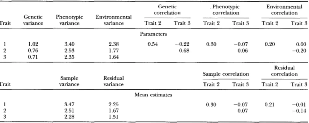
TABLE 4

S u m m a r y parameters and mean statistics of traits for the simulation example in Table 3

Genetic Phenotypic Environmental

Genetic Phenotypic Environmental correlation correlation correlation

Trait variance variance variance Trait 2 Trait 3 Trait 2 Trait 3 Trait 2 Trait 3

Parameters

1 1.02 3.40 2.38 0.54 -0.22 0.30 -0.07 0.20 0.00

2 0.76 2.53 1.77 0.68 0.06 -0.20

3 0.71 2.35 1.64

Residual Sample correlation correlation

Sample Residual

Trait variance variance Trait 2 Trait 3 Trait 2 Trait 3

Mean estimates

1 3.47 2.25 0.30 -0.07 0.21 -0.01

2 2.51 1.67 0.07 -0.14

3 2.28 1.51

4).

Sample means, variances and correlation coeffi-

cients averaged over 100 replicates are also listed in

Table 4. It is interesting to observe that the observed

(averaged) residual variances and correlations are very close to the expected environmental variances and cor- relations, as in the analysis most of the genetic variation is absorbed by markers fitted in the model.

Seven methods of QTL mapping were performed on

each simulated data set at every 1 cM on the chromo-

some. These include the following: joint mapping for

three traits (5-123 ) ,joint mapping for each pair of traits

(5-12,J-13 and 5-23) , and separate mapping for each

trait ( S1, $2 and $ 3 ) . Simply for the convenience of

discussion, in mapping except for the flanking markers,

all other markers are fitted in the model to control the genetic background because markers are evenly distrib-

uted and widely separated. We used x:.05/15,7 = 21.4,

x0,05/15,5

=

17.7,

and

xi.os/15,3

= 13.6 as the critical values of the test for the three levels of mapping.

Summary estimates of QTL positions and effects by

the seven mapping methods are given in Table 3, and

the observed power of detection of QTL are given in

Table 5. The statistics given in Tables 3 and 5 are sum-

marized from 100 replicates for three QTL regions sep-

arately. Although three QTL are assumed to be located

on the same chromosome, they are widely separated.

TABLE 5

Observed statistical power (proportion of significant replicates over all replicates) of seven methods of QTL

mapping from 100 replicates of simulations

2

QTL 5-123 5-12 5-13 5-23 $1 $2 S 3 S-123

1 0.80 0.78 0.51 0.64 0.46 0.64 0.04 0.78 2 0.79 0.37 0.36 0.84 0.00 0.39 0.41 0.64 3 0.89 0.51 0.84 0.64 0.42 0.00 0.64 0.79

Also because of the composite interval mapping used

in analysis, tests in different regions are statistically inde-

pendent ( ZENG 1993), so that the statistical power and

sampling variance of estimates can be calculated sepa- rately for three QTL at and around the intervals sur-

rounding the QTL. In Table 5 , $123 denotes the overall

performance of the three separate mappings, and its power was calculated as the frequency of the detection of the QTL by at least one of the three separate m a p

pings. It is seen that the power of 5-123 in this case is

higher than that of S-123 for all three QTL. This shows

that some QTL with relatively small effects may be

missed by separate mappings on different traits but de-

tected by joint mapping that combined information

from different traits. The power of 5-12 is very close to

that of 5-123 on QTL 1. This is because QTL 1 has

effects mainly on traits 1 and 2, and just a small effect

on trait 3. The exclusion of trait 3 in 5-12 only slightly

affects the power of detection of the QTL. This also shows that small pleiotropic effects on additional traits included in the joint mapping may be large enough to compensate the lose of power due to the increase of

the critical value. The powers of QTL detection by J -

12,J-13 and 5-23 are generally comparable to the sizes

of pleiotropic QTL effects involved. 5-23, however, tends

to have relatively higher power. This is because the

pleiotropic effects of three QTL on traits 2 and 3 are

all in the same direction and the environment correla-

tion is negative (see APPENDIX A )

.

Means and SDs of estimates (over all replicates) of

QTL positions and effects by different methods are also

given in Table 3. All estimates seem to be relatively

unbiased. In general, the precision of estimation of

QTL positions and effects by 5-123, as indicated by SDs,

is better than other methods. Particularly, the joint anal-

Mapping QTL on Multiple Traits

TABLE 6

Parameters of QTL positions and effects and their estimates in a single replicate of simulation by the joint mapping on two traits (J-12) and the separate mapping on each trait ($1 and S2)

Additive effect Dominance effect

Position Likelihood

QTL ( C M ) Trait 1 Trait 2 Trait 1 Trait 2 ratio

Parameters

1 54 - 1.36 - 1.44 1.28 1.35

2 114 -1.16 0.75

3 128 1.30 0.49

Estimates by 5-12

1 57 - 1.03 - 1.34 1.36 1.42 66.73

2/ 3 125 -0.82 1.31 -0.35 0.52 37.49

Estimates by S1

1 55 -1.05 1.42 28.07

2 110 -0.75 1.16 15.01

Estimates by $2

1 61 -1.22 1.24 51.95

3 127 1.34 0.45 24.24

variance of estimates of QTL positions. Sampling vari-

ances of estimates of QTL positions by 5-123 are consis-

tently smaller than those by other analyses, except of

that for QTL 3 by 5-13 and for QTL 2 by 5-23 in which

cases two trait analyses have some particular advantages as noticed above.

Pleiotropy us. close linkage with one replicate: We also performed a simulation to test close linkage of two nonpleiotropic QTL against pleiotropy of a common

QTL. In this example, one chromosome with 11 mark-

ers in 10 marker intervals, each with 15 cM, was simu-

lated. Three QTL, one pleiotropic and two nonpleiotro- pic, were assumed to affect two traits with parameters

given in Table 6. The heritability for each trait is 0.4.

(The effects of QTL are undoubtedly very large.) The sample genetic, environmental and phenotypic correla-

tions are 0.42, 0.2 and 0.29, respectively. The sample

size is 300.

The results of joint mapping (5-12) and separate

mappings ( S-1 and $2) in one replicate are presented

in Table 6 and Figure 1 . At least two major QTL are

indicated by the analyses. There is some evidence from

separate mappings that there might be two nonpleiotro-

pic QTL in the region between 105 and 135 cM with

each showing a significant effect on one trait only. To

test this hypothesis, the test of pleiotropy 11s. close link-

age was performed in the two major regions that show significant effects on the traits for comparison: one be-

tween 45 and 75 cM and one between 105 and 135 cM.

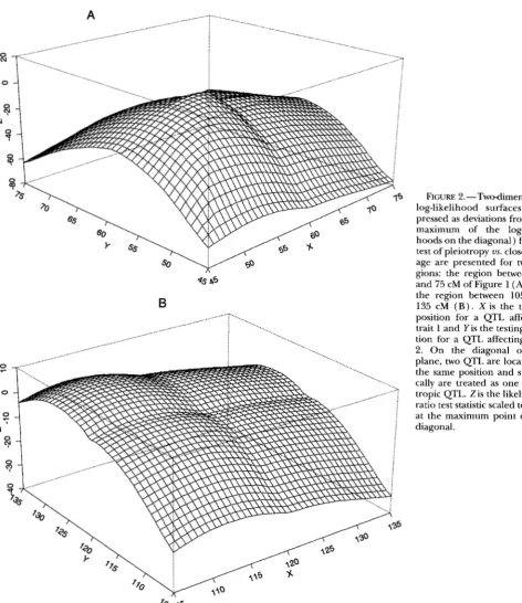
The results are plotted in Figure 2.

In Figure 2, the two-dimensional log-likelihood sur-

face (as deviations from the maximum of the log-likeli-

7 0

8 0

0 50

.rl

c,

m

3

40 Ld c,

30

c,

rn

4 Q) 20

E

crl

10

0

1121

A

A

A

I I I 1 I I I I I

-1

0 15 30 45 80 75 90 105 120 135 150

Testing

position

(cM)

FIGURE 1. -A simulation example of QTL mapping on two traits from an F2 population. Likelihood ratio test statistics are calculated and plotted at every 1 cM position of a chromosome for three mapping methods. 5-12 is the joint mapping on two

1122 C. Jiang and Z . 3 . Zeng

8

__.. ___..__...

-y$@$

..."

hoods on the diagonal) is presented. In this analysis, unlike joint mapping and the separate mappings that used all but flanking markers for background control,

only markers 1-3 and

7-11

are used in the model for

background control in Figure 2A, and only markers 1

-

7

and 11 are used for background control in Figure

2B.

On this two-dimensional surface, the diagonal elements represents null hypotheses of one pleiotropic QTL, and the offdiagonal elements represent alternative hypoth-

eses of two nonpleiotropic QTL. The likelihood ratio

FIGURE 2.-Two-dimensional log-likelihood surfaces (ex- pressed as deviations from the maximum of the log-likeli- hoods on the diagonal) for the test of pleiotropy us. close link- age are presented for two re- gions: the region between 45 and 75 cM of Figure 1 ( A ) and the region between 105 and 135 cM ( B ) . X is the testing position for a QTL affecting trait 1 and Yis the testing posi- tion for a QTL affecting trait 2. On the diagonal of X-Y plane, two QTL are located in the same position and statisti- cally are treated as one pleio- tropic QTL. Z is the likelihood ratio test statistic scaled to zero at the maximum point of the diagonal.

test is performed at the maximum of the surface against

the maximum of the diagonals. This likelihood ratio is

0.53 for Figure 2A at the position 56 cM for trait 1 and

57 cM for trait 2 (the maximum diagonal is at 57 cM) ,

which is clearly not significant, and 7.26 for Figure 2B

at the position 111 cM for trait 1 and 126 cM for trait

2 (the maximum diagonal is at 125 cM)

,

which is sig-

nificant at 0.01 level (for chi-square distribution with

one degree of freedom). There is clear evidence to

Mapping QTL on Multiple Traits

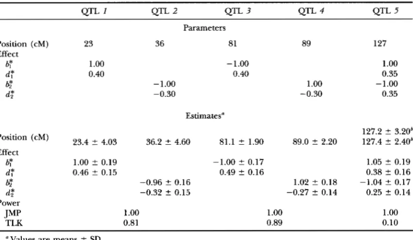
TABLE 7

Parameters of Q l T positions and effects and their estimates over 100 replicates of simulation under the close linkage model

1123

QTL 1 QTL 2 QTL 3 QTL 4 QTL 5

Position (cM)

Effect

b$

d:

@

d,*

Position (cM)

Effect

b?

dT

@

&

JMP Power

TLK

Parameters

23 36 81 89

1

.oo

-1.00

0.40 0.40

-1.00 1

.oo

-0.30 -0.30

Estimates"

23.4 2 4.03 36.2 2 4.60 81.1 ? 1.90 89.0 t 2.20

1.00 ? 0.19 -1.00 ? 0.17

0.46 2 0.15 0.49 2 0.16

-0.96 2 0.16 1.02 % 0.18

-0.32 2 0.15 -0.27 2 0.14

1

.oo

1

.oo

0.81 0.89 127

1

.oo

0.35 -1.00

0.35

127.2 2 3.20b 127.4 t 2.40b

1.05 2 0.19 0.38 t 0.16

0.25 2 0.14

1

.oo

0.10 -1.04 % 0.17

"Values are means 2 SD.

Here the estimates of position of QTL 5 are ~ v e n for each trait separately (under the nonpleiotropic

model) to indicate the closeness of the kstimates.

around 111 cM showing a significant effect on trait 1

and one located around 126 cM showing a significant

effect on trait

2.

The maximum positions of diagonals in Figure 2 are the same maximum positions under the joint mapping

in Figure 1 and Table 6. The maximum positions of

offdiagonals in Figure 2 are also very close to the maxi- mum positions indicated by the separate mappings (Ta-

ble 6 ) . As discussed above, in practice this twodimen-

sional search for the best fit of two nonpleiotropic QTL is unnecessary, although the two-dimensional surface is more illuminating. The test can be constructed at the

peak suggested by joint mapping for the null hypothesis

and at or around the peak suggested by separate map- pings for the alternative hypothesis. This is clearly sup- ported by the results of Figure 2. These are, however, the results of simulation in one replicate.

Pleiotropy us. close linkage with multiple repli- cates: To show the behavior of the test statistic, we also performed simulations and tests with multiple repli- cates. The parameters of this simulation are, however,

different from the above example and are shown in

Table 7. In this simulation, one chromosome with 16 uniformly distributed markers in 15 10-cM marker in- tervals was simulated. Five QTL, one pleiotropic and

four nonpleiotropic, are assumed to affect two traits

with effects and positions listed in the table. The mag- nitudes of QTL effects are assumed to be the same for additive effects and slightly different for dominant

effects. In this way, the statistical power of the test is

comparable for different QTL. Heritabilities of the two

traits are all assumed to be 0.6 and the environmental

correlation coefficient between the traits is 0.2. Sample size is 150 and the number of replicates of simulation is 100.

For each replicate, the joint mapping is first per- formed using the procedure stated above. In the joint

mapping, QTL 1 and

2

can be detected only as one

QTL and so are QTL 3 and

4.

Therefore, only three

QTL are indicated by the joint analysis, and they are significant in all the replicates (with the estimated

power of 1 in Table

7 ) .

Again, by using the result of

ZENG ( 1994), the critical value of the joint mapping is

set to be

17.7,

which corresponds to the chi-square value

with 5 degrees of freedom at the significance level of

(0.05

/

15= ) 0.0033. The separate mappings, however,

failed to detect some QTL in a few replicates (results

not shown)

.

The corresponding critical value used in

the separate mappings is 13.6.

Statistical tests for the hypotheses of pleiotropy us.

close linkage are then performed in the three regions indicated by the joint mapping. The observed powers

of the test are given in Table

7.

The power of the test

for QTL 1 and 2 is 0.81, which is slightly lower than

that for QTL 3 and 4. This may be because QTL 1 and

2

are relatively more distant from nearby markers than

QTL 3 and 4 that are only 1 cM away from the respective