INVESTIGATION
Emergent Neutrality in Adaptive Asexual Evolution
Stephan Schiffels,*,1Gergely J. Szöllosi,} †,1Ville Mustonen,‡and Michael Lässig*,2 *Institut für Theoretische Physik, Universität zu Köln, 50937 Köln, Germany,†Centre National de la Recherche Scientifique, UMR 5558–Laboratoire de Biométrie et Biologie Évolutive, Université Claude Bernard, Lyon 1, France, and‡Wellcome Trust Sanger Institute, Hinxton, Cambridge, CB10 1SA, United Kingdom
ABSTRACT In nonrecombining genomes, genetic linkage can be an important evolutionary force. Linkage generates interference interactions, by which simultaneously occurring mutations affect each other’s chance offixation. Here, we develop a comprehensive model of adaptive evolution in linked genomes, which integrates interference interactions between multiple beneficial and deleterious mutations into a unified framework. By an approximate analytical solution, we predict thefixation rates of these mutations, as well as the probabilities of beneficial and deleterious alleles atfixed genomic sites. Wefind that interference interactions generate a regime of emergent neutrality: all genomic sites with selection coefficients smaller in magnitude than a characteristic threshold have nearly randomfixed alleles, and both beneficial and deleterious mutations at these sites have nearly neutralfixation rates. We show that this dynamic limits not only the speed of adaptation, but also a population’s degree of adaptation in its current environment. We apply the model to different scenarios: stationary adaptation in a time-dependent environment and approach to equilibrium in afixed environ-ment. In both cases, the analytical predictions are in good agreement with numerical simulations. Our results suggest that interference can severely compromise biological functions in an adapting population, which sets viability limits on adaptive evolution under linkage.
P
OPULATIONS adapt to new environments byfixation of beneficial mutations. In linked sequence, simultaneously occurring mutations interfere with each other’s evolution and enhance or reduce each other’s chance of fixation in the population. We refer to these two cases as positive and negative interference. Several classical studies have shown that interference can substantially reduce the speed of adaptation in large asexual populations (Fisher 1930; Muller 1932; Smith 1971; Felsenstein 1974; Barton 1995; Gerrish and Lenski 1998). Linkage effects are weaker in sexual populations, because they are counteracted by re-combination.Microbial evolution experiments provide a growing amount of data on adaptive evolution under linkage (de Visser et al.1999; Rozen et al.2002; de Visser and Rozen 2006; Desai and Fisher 2007; Perfeitoet al. 2007; Silander et al. 2007; Kao and Sherlock 2008; Barrick et al. 2009; Betancourt 2009; Kinnersleyet al.2009), and similar data
are available for adaptive evolution in viral systems (Bush et al.1999; Rambautet al.2008; Neher and Leitner 2010). Modern deep sequencing opens these systems to genomic analysis and poses new questions: How does a continuously changing environment such as the human immune chal-lenge shape the genome of the seasonal influenza virus? How does the fitness of a bacterial population increase in a new environment? To answer such questions, we need to explain how a population and its current fitness values evolve in a time-dependent ecology and fitness landscape and what are the rates of beneficial and deleterious changes observed in this process. Thus, we need to describe the adaptive process in an explicitly genomic context.
In this article, we develop a genomic model of adaptation under linkage, which establishes the conceptual framework to analyze such data. Our model links theadaptive process, which changes the frequencies of beneficial and deleterious alleles at polymorphic sites, to the genome state, which includes the distribution of beneficial and deleterious alleles at fixed sites. It is the genome state that determines the
fitness of a population in its current environment. We show that interference interactions can drastically affect process and state in large asexual populations: Adaptation generates beneficialdrivermutations, but a substantial fraction of al-lele changes arepassengermutations, whose chance offi xa-tion depends only weakly on their selecxa-tion coefficient. Thus,
Copyright © 2011 by the Genetics Society of America doi: 10.1534/genetics.111.132027
Manuscript received June 30, 2011; accepted for publication September 8, 2011 Available freely online through the author-supported open access option. Supporting information is available online at http://www.genetics.org/content/ suppl/2011/09/16/genetics.111.132027.DC1.
1These authors contributed equally to this work.
2Corresponding author: Institut für Theoretische Physik, Universität zu Köln, Zülpicher
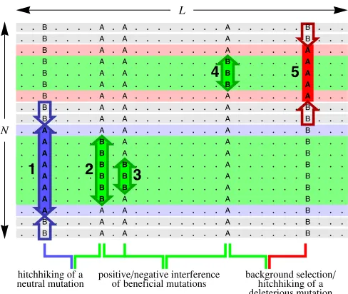
a near-neutral dynamic of mutations emerges from suffi -ciently strong interference interactions. This effect causes a—potentially large—fraction of genomic sites to have nearly random fixed alleles, which do not reflect the direction of selection at these sites. Thus, interference interactions not only reduce the speed of adaptation, but also degrade the genome state and the population’sfitness in its current envi-ronment. The joint dynamics of driver and passenger muta-tions have consequences that may appear counterintuitive: deleterious substitutions of a given strength can have a rate increasing with population size, and beneficial substitutions can have a rate decreasing with population size. This behav-ior is contrary to unlinked sites evolving under genetic drift. The complexity of genomic linkage and of interference interactions is reflected by the long history of the subject in population genetics literature, which dates back to Fisher and Muller (Fisher 1930; Muller 1932). Their key observa-tion is that in the absence of recombinaobserva-tion, two mutaobserva-tions can both reachfixation only if the second mutation occurs in an individual that already carries thefirst. In other words, mutations occurring in different individuals interfere with one another. Interference inevitably causes a fraction of all mutations to be lost, even if they are beneficial and have already reached substantial frequencies in the population (i.e., have overcome genetic drift). Following a further sem-inal study, the interference between linked mutations is commonly referred to as the Hill–Robertson effect (Hill and Robertson 1966). This term is also used more broadly to describe the interplay between linkage and selection: in-terference interactions reduce the fixation probability of beneficial mutations and enhance that of deleterious ones. Hence, they reduce the effect of selection on substitution rates (Felsenstein 1974; Barton 1995), but for which muta-tions, and by how much? A number of theoretical and ex-perimental studies have addressed these questions and have led to a quite diverse picture of particular interaction effects. These effects, which are sketched in Figure 1, include (i) interference between strongly beneficial mutations (clonal interference and related models) (Gerrish and Lenski 1998; Orr 2000; Rouzine et al. 2003; Wilke 2004; Desai et al. 2007; Park and Krug 2007, Hallatschek 2011) and between weakly selected mutations (McVean and Charlesworth 2000; Comeron and Kreitman 2002; Comeronet al.2008), (ii) the effects of strongly beneficial mutations on linked neutral mutations (genetic hitchhiking, genetic draft) (Smith and Haigh 1974; Barton 2000; Gillespie 2001; Kim and Stephan 2003; Hermisson and Pennings 2005; Andolfatto 2007), and (iii) the effects of strongly deleterious mutations on linked neutral or weakly selected mutations (background selection) (Charlesworth et al. 1993; Charlesworth 1994, 1996; Kim and Stephan 2000; Bachtrog and Gordo 2004; Kaiser and Charlesworth 2009).
Adaptive evolution under linkage contains all of these processes, and the model developed in this article integrates positive and negative interference, background selection, and hitchhiking into a unified treatment of multiple
in-teracting mutations. Specifically, the model describes the adaptive evolution of a finite asexual population, whose individuals have nonrecombining genotypes of finite length. Evolution takes place by mutations, genetic drift, and selection given by a genomicfitness function, which is specified by the distribution of selection coefficients be-tween alleles at individual sequence sites and may be explicitly time dependent. The evolving population is described by its genome state, i.e., by the probabilities of beneficial and deleterious alleles atfixed sites. The genome state influences the rate and distribution of selection
coef-ficients for mutations in individuals: the better the popula-tion is adapted, the more sites arefixed at beneficial alleles and the more novel mutations will be deleterious. Thus, the scope of our genomic model goes beyond that of pre-vious studies that analyze the statistics of substitutions given the rate and the effects of mutations as fixed input parameters (Gerrish and Lenski 1998; Desai et al. 2007; Park and Krug 2007). In particular, our model naturally includes nonstationary adaptation, i.e., processes in which the distribution of selection effects for mutations becomes itself time dependent.
The key derivation of this article concerns the effects of interference interactions on the evolution of the genome state. We develop an approximate calculus for multiple simultaneous mutations. Specifically, we determine how the
fixation probability of a specific target mutation is affected by positive and negative interference of other mutations. Since the target mutation can, in turn, act as interfering mutation, we obtain an approximate, self-consistent sum-mation of interference interactions between all co-occurring mutations. We show that these interactions partition the adaptive dynamics into strongly beneficial driver mutations, whichfix without substantial interference, and beneficial or deleterious passenger mutations, which suffer strong posi-tive or negaposi-tive interference.
Our analytical approach differs from the two classes of models analyzed in previous work. The clonal interference calculus (Gerrish and Lenski 1998) focuses on the dynamics of driver mutations, but it does not consider passenger mutations and neglects the effects of multiple co-occurring mutations. On the other hand, the traveling-wave approach assumes an ensemble of many co-occurring mutations, which have the same or a similar selective effect (Rouzine et al.2003; Desaiet al.2007). The adaptive processes stud-ied in this article—and arguably those in many real systems— take place in linked genomes with more broadly distributed selection coefficients and differ from both model classes: they are governed by interference interactions between multiple, but few strongly beneficial substitutions and their effect on weaker selected alleles. We show that this leads to intermit-tentfitness waves, which have large fluctuations and travel faster than fitness waves with deterministic bulk. This sce-nario and the results of our model are supported by simula-tions over a wide range of evolutionary parameters, which includes those of typical microbial evolution experiments. Its range of validity and the crossover to other modes of evolu-tion are detailed in theDiscussion.
We analyze our model and its biological implications for two specific scenarios of adaptive evolution. The first is a stationary adaptive process maintained by an explicitly time-dependent fitness“seascape”, in which selection
coef-ficients at individual genomic sites change direction at a con-stant rate (Mustonen and Lässig 2007, 2008, 2009). Such time dependence of selection describes changing environ-ments, which can be generated by external conditions, mi-gration, or coevolution. An example is the antigen–antibody coevolution of the human influenza virus (Bushet al.1999). Our model predicts the regime of emergent neutral genomic sites, the speed of adaptation, and the population’s degree of adaptation in its current environment. The second scenario is the approach to evolutionary equilibrium in a staticfitness landscape, starting from a poorly adapted initial state. This case describes, for example, the long-term laboratory evo-lution of bacterial populations in a constant environment (Barrick et al. 2009). The predictions of our model are now time dependent: the regime of emergent neutral sites
and the speed of adaptation decrease over time, while the degree of adaptation increases.
This article has two main parts. In the first part, we introduce a minimal genomic model for adaptation under linkage and present its general solution. In the second part, we discuss the application of the model to the scenarios of stationary adaptation and approach to equilibrium. In the Discussion, we draw general biological consequences and place our model into a broader context of asexual evolution-ary processes.
Minimal Model for Adaptive Genome Evolution
Wefirst introduce our model of genome evolution, as well as two key observables of the evolutionary process: the degree of adaptation, which measures thefitness of a population in its current environment, and the fitnessflux, which we use as a measure of the speed of adaptation. We then calculate the fixation probability of beneficial and deleterious muta-tions and show, in particular, the emergence of neutrality.
Genome state and degree of adaptation
We consider an evolving asexual population offixed sizeN, in which each individual has a genome of lengthLwith two possible alleles per site. Our minimal fitness model is addi-tive and fairly standard: each site is assigned a nonnegaaddi-tive selection coefficient f, which equals the fitness difference between its beneficial and its deleterious allele. The site selection coefficients are drawn independently from a nor-malized distribution r(f), which is parameterized by its meanf and a shape parameter k[we use a Weibull distri-bution, which has a tail of the formrðfÞ exp½2ðf=fÞk; see section 6 ofsupporting information,File S1for details]. In section 7.4 of File S1, we introduce an extension of the
fitness model with simplefitness interactions (epistasis) be-tween sites, and we show that such interactions do not affect the conclusions of this article.
Point mutations between nucleotides take place with a uniform ratem. We assume that the population evolves in the low-mutation regimemN>1, in which one of the two nucleotide alleles isfixed in the population at most sequence sites, and a fractionmNor less of the sites are polymorphic. In this regime, the two-allele genome model adequately describes the evolution of a genome with four nucleotides, because polymorphic sites with more than two nucleotides occur with negligible frequency. The genome state of the population is then characterized by the probability that afixed site with selection coefficientfcarries the beneficial allele,lb(f), or the probability that it carries the deleterious
allele,ld(f). We use the familiar weak-mutation
approxima-tion lb(f) + ld(f) = 1 (this approximation neglects the
probability that a site is polymorphic, which is of ordermN log N). The selection-dependent degree of adaptation, which is defined as a(f) = lb(f) 2 ld(f), varies between
with probability 1. For example, a single locus with two alleles and time-independent selection coefficient f has
a(f) = tanh(Nf) at evolutionary equilibrium (Kimura 1962; Mustonen and Lässig 2007).
In a similar way, we define the degree of adaptation in the entire genome as the weighted average over all sites,
a¼1
f
ZN
0
rðfÞdf f½lbðfÞ2ldðfÞ: (1)
This summary statistic can be written in the form a = (F2F0)/(Fmax2F0), whereFis the Malthusian population fitness,F0is thefitness of a random genome, andFmaxis the fitness of a perfectly adapted genome. Hence,avaries be-tween 0 for a random genome and 1 for a perfectly adapted genome, and 12ais a normalized measure of genetic load (Haldane 1937; Muller 1950). For an adaptive process, the lag of the genomic state behind the currentfitness optimum can lead to a substantial reduction of a (Haldane 1957; Smith 1976), which is larger than the reduction due to mu-tational load (of order m=f). In the following, we useato measure thefitness cost of interference.
Mutations and speed of adaptation
A genomic site of selection coefficientfevolves by beneficial mutations with selection coefficients=f.0 and by dele-terious mutations with selection coefficient s = 2f , 0 (recall that f is, by definition, nonnegative). Hence, the distributions of beneficial and deleterious alleles at fixed sites, lb,d(f), determine the genome-wide rate of
muta-tions with a given selection coefficient occurring in the population,
UðsÞ ¼
mNLrðsÞldðsÞ ðs.0; beneficial mutationsÞ;
mNLrðjsjÞlbðjsjÞ ðs,0; deleterious mutationsÞ: (2)
The total rates of beneficial and deleterious mutations are obtained by integration over all positive and negative selection coefficients,Ub¼
RN
0dsUðsÞandUd¼
R0
2NdsUðsÞ. The dis-tribution U(s) is conceptually different from the distribu-tionr(s) of selection coefficients at genomic sites, because it depends on the genome statelb,d(f). Therefore, both the
shape of U(s) and the total ratesUb,dare in general time
dependent, even if r(f) is fixed. A similar coupling be-tween the distribution U(s) and the adaptive state of the population has been discussed previously, for example, in the context of Fisher’s geometrical model (Martin and Lenormand 2006; Tenaillon et al. 2007; Waxman 2007; Rouzineet al.2008). For stationary evolution with an ex-ponentialr(f), wefind the distributionU(s) of beneficial mutations (s .0) is approximately exponential as well, which is in accordance with the form suggested by pre-vious studies (Gillespie 1984; Imhof and Schlotterer 2001; Orr 2003; Rokytaet al.2005; Kassen and Bataillon 2006; Eyre-Walker and Keightley 2007; MacLean and Buckling 2009).
The selection-dependent substitution rate is given by the product of the mutation rate and probability offixationG(s) of a mutation with selection coefficients,
VðsÞ ¼GðsÞUðsÞ: (3)
For unlinked sites, the fixation probability is given by Kimura’s classical result, G0(s) = (1 2 exp[22s])/(1 2
exp[22Ns]) (Kimura 1962). Computing this probability for linked sites is at the core of this article: G(s) depends not only on the selection strengthsand population size N, but also on the interference interactions between co-occurring mutations shown in Figure 1.
To measure the speed of adaptation contributed by sites with selection coefficientf, we define thefitnessfluxF(f) = f[V(f)2V(2f)]. The totalfitnessflux
F¼
ZN
0
df FðfÞ ¼
ZN
2Nds sVðsÞ ¼VsV (4)
is simply the product of the total rate V and the average selection coefficient sV of substitutions (Mustonen and Lässig 2007). If evolution is adaptive, it can be shown that
F is always positive (Mustonen and Lässig 2010), which reflects an excess of beneficial over deleterious substitutions. In the following, we use F to measure the reduction in speed of adaptation due to interference (Gerrish and Lenski 1998).
Adaptive dynamics
Changes in selection and substitutions together deter-mine the change of the genome state,
dlbðfÞ
dt ¼ 2
dldðfÞ dt ¼ 1
LrðfÞ½VðfÞ2Vð2fÞ þg½ldðfÞ2lbðfÞ ;
(5)
which, in turn, determines the substitution rates V(s) by Equations 2 and 3. These coupled dynamics admit an itera-tive solution, once we have computed the fixation prob-ability G(s) (see below). Equation 5 can be expressed as a relation between the selection-dependent fitness flux
F(f), the degree of adaptationa(f), and its time derivative,
FðfÞ ¼LrðfÞf
1 2
daðfÞ
dt þgaðfÞ
: (6)
Hence, a population’sfitness in a time-dependent environ-ment increases byfitnessflux and decreases by changes of thefitness seascape. A similar relation follows for the total
fitnessfluxF(Equation 4) and the genome-averaged degree of adaptation (Equation 1),
F¼Lf
1 2
da
dtþga
: (7)
In the second part of this article, we analyze these dynamics in two specific scenarios.
Stationary adaptation under time-dependent selection:
In this case, the genome state becomes static, dlb,d/dt =
da/dt = 0. This state is determined by the fixation proba-bilitiesG(s) and the selection flip rateg,
lbðfÞ ¼12ldðfÞ ¼
NGðfÞ þg= m
NGðfÞ þNGð2fÞ þ2g= m (8)
(Mustonen and Lässig 2007). The stationary fitness flux becomes proportional to the degree of adaptation,
F¼fgLa ðstationary adaptationÞ; (9)
that is, the actualfitness fluxF is only a fractionaof the maximalfluxf
gLrequired for perfect adaptation.
Approach to equilibrium under time-independent selec-tion: In a static fitness landscape (g = 0), adaptation is the approach to a mutation–selection–drift equilibrium state. In this case, the fitness flux is simply the change in fitness,
F¼dF
dt¼ f L
2 da
dt ðapproach to equilibriumÞ; (10)
that is, the populationfitness increases with time toward its equilibrium value.
Fixation probability of interacting mutations
The missing piece in the coupled dynamics of substitutions and genomic state (Equations 2, 3, and 5) is the fixation probability G(s). Consider a target mutation with origina-tion time t and selection coefficient s, which is subject to interference by a mutation with origination timet9and a se-lection coefficient s9 larger in magnitude, js9j . jsj; this hierarchical approximation is detailed further below. We classify pairwise interactions between interfering and target mutations by three criteria:
i. Temporal order: The interfering mutation originates either at a timet9 ,t(we call this case background interfering mutation) or at a timet9 .t(future interfering mutation).
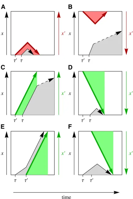
Figure 2 Interference time series diagrams. A target mutation with orig-ination timetand frequencyx(t) (black arrow) is subject to a stronger interfering mutation with origination timet9and frequencyx9(t) (colored arrow). The interactions between this pair of mutations can be classified as follows: (A and B)Interference by a deleterious background mutation
ii. Direction of selection on the interfering mutation: Deleterious or beneficial.iii. Allele association: The target mutation may occur on the ancestral or the new allele of a background interfering mutation; similarly, a future interfering mutation may occur on the ancestral or the new allele of the target mutation. Figure 2 shows this classification: a target mutation interacts with a deleteri-ous background interfering mutation (Figure 2, A and B), with a beneficial background interfering mutation (Figure 2, C and D), and with a beneficial future interfering mutation (Figure 2, E and F). The case of deleterious future interfering mutations is not shown, because their contribution to thefixation probability is negligible.
As a first step, we evaluate the conditional fixation proba-bility of a target mutation,G(s,t| s9,t9), for each of the cases of Figure 2, A–F, and for given selection coefficientss,
s9 and origination times t, t9. This step is detailed in the Appendix. The net contribution of deleterious background (Figure 2, A and B) is found to be small, because the re-duction infixation probability for association with the dele-terious allele is offset by an enhancement for association with the beneficial allele. The relationship of this result to previous studies of background selection is discussed in sec-tion 1 ofFile S1. Beneficial background mutations (Figure 2, C and D) retain a net effect on thefixation probability of the target mutation. The largest effect turns out to arise from future interfering mutations (Figure 2, E and F).
We now derive an approximate expression for the total
fixation probability of a target mutation on the basis of pair interactions with multiple interfering mutations. Clearly, a straightforward “cluster expansion”makes sense only in a regime ofdiluteselective sweeps at sufficiently low rates of beneficial mutations, where the interference interactions of Figure 2, C–F, are infrequent. However, we are primarily interested in adaptive processes under linkage in the dense-sweep regime at high rates of beneficial mutations, which generates strongly correlated clusters of fixed muta-tions nested in each other’s background (the crossover be-tween these regimes is further quantified below). We treat the dense-sweep regime by an approximation: each sweep is associated with a uniquedriver mutation, which is the stron-gest beneficial mutation in its cluster. The driver mutation itself evolves free of interference, but it influences other mutations by interference; that is, we neglect the feedback of weaker beneficial and deleterious mutations on the driver mutation. In this hierarchical approximation, the coherence time of a sweep is set by the fixation time of its driver mutation, tfix(s) = 2 log(2Ns)/s (see section 2 of File S1). The sweep rate becomes equal to the rate of driver mutations, Vdrive(s), and is given by the condition that no
stronger selective sweep occurs during the interval tfix(s).
Hence, we obtain a self-consistent relation,
VdriveðsÞ ¼pdriveðsÞG0ðsÞUðsÞ (11)
with
pdrive ðsÞ ¼exp
2tfixðsÞ
ZN
s
VdriveðzÞdz
; (12)
which can be regarded as a partial summation of higher-order interference interactions characteristic of the dense-sweep regime (see theAppendixfor details). These expressions and the underlying hierarchical approximation are similar to the model of clonal interference by Gerrish and Lenski (1998). This model determines an approximation of the sweep rate, VGL(s), by requiring that nonegativeinterference by a future
interfering mutation occurs (see below for a quantitative com-parison with our model).
Consistent with the hierarchical approximation, we can interpret the diagrams of Figure 2, C–E, as effectivepair in-teractions between a target mutation and a selective sweep, which is represented by its driver mutation. The target mu-tation can strongly interact with two such sweeps, the last sweep before its origination (with parameters s9 . sand
t9 .t) and thefirst sweep after its origination (with param-eters t99 . t and s99 . s). These two sweeps affect the
fixation probabilityG(s) in a combined way: the target mu-tation can befixed only if it appears on the background of the last background sweep and if it is itself the background of thefirst future sweep. The resulting conditional fixation probability of the target mutation, G(s,tjs9,t9, s99,t99), is a straightforward extension of the form obtained for a single interfering mutation. The full fixation probability G(s) is then obtained by integration over the selection coefficients s9, s99 with weights Vdrive(s9) and Vdrive(s99)
and over the waiting timest2t9,t99 2t. This calculation and the result for G(s), Equation A6, are given in the Appendix.
The fixation probability can be expressed as the sum of driver and passenger contributions,
GðsÞ ¼pdriveðsÞG0ðsÞ þ ½12pdriveðsÞGpassðsÞ: (13)
A passenger mutation fixes predominantly by interference from other stronger mutations, which results in a fixation probabilityGpass (see Equation A8). The arguments leading
to Equations 11 and 12 must be modified, if the distribution of selection coefficientsp(f) falls off much faster than expo-nentially (Fogle et al. 2008). In that case, we can still de-scribe the fixation probability of a target mutation as the result of interference interaction with the closest past and future sweep, but these sweeps may contain several driver mutations of comparable strength (seeDiscussion). The sys-tem of Equations 2, 3, 8, 11, 12, and 13 can be solved numerically using a straightforward iterative algorithm, which is detailed in section 4 ofFile S1.
Emergent neutrality
For mutations of sufficiently weak effect, the fixation probability takes the particularly simple form
GðsÞ≃GpassðsÞ≃G0
s
2N~s for 2~s,s,s~
where the neutrality thresholds~is given by the total sweep rateVdrive¼
RN
0 VdriveðzÞdz,
~
s¼ 1
2NþVdrive (15)
(see the Appendix). These are the central equations of this article. They show how neutrality emerges for strong adap-tive evolution under linkage. Specifically, the relation fors~
delineates two dynamical modes: the dilute sweep mode (Vdrive ≲ 1/2N), where the neutrality threshold is set by
genetic drift to the Kimura values~≃1=2N(Kimura 1962), and the dense sweep mode (Vdrive ≲ 1/2N), where
interfer-ence effects generate a broader neutrality regime with ~
s≃Vdrive. The transition between these modes marks the
onset of clonal interference as defined in previous work (Wilke 2004; Park and Krug 2007). For stationary adapta-tion in a time-dependentfitness seascape, the upper bound Vdrive≃gLproduces the estimate 2NgL.1 for the crossover
from dilute to dense sweeps. However, Equations 14 and 15 remain valid for nonstationary adaptation, where the neu-trality threshold ~sbecomes time dependent (see below).
In summary, interference interactions in the dense-sweep mode produce the following selection classes of mutations and genomic sites.
Emergent neutrality regime: Mutations with selection coefficients2~s,s,s~fix predominantly as passenger muta-tions. Their near-neutral fixation probability (Equation 14) is the joint effect of positive and negative interference. Com-pared to unlinked mutations,G(s) is reduced for beneficial mutations and enhanced for deleterious mutations. Accord-ingly, sites with selection coefficientsf,s~have near-random probabilities of their alleles.
Adaptive regime:Mutations with effectss.s~have afixation rate significantly above the neutral rate and, hence, account for most of thefitnessflux. Moderately beneficial mutations ðs≳s~Þ still fix predominantly as passengers, whereas strongly beneficial mutations ðs?~sÞ are predominantly drivers. Hence, thefixation rate increases to values of order G0(s)≃2s, which are characteristic of unlinked mutations.
Accordingly, sites withf.s~evolve toward a high degree of adaptation.
Deleterious passenger regime: Mutations with s,2s~ can
fix by positive interference,i.e., by hitchhiking in selective sweeps. This effect drastically enhances thefixation rate in comparison to the unlinked case. It follows the heuristic ap-proximation GðsÞ GpassðsÞ expð2jsj=~sÞ, which extends
the linear reduction in the effective strength of selection (Equation 14) obtained in the emergent neutrality regime.
Applications to Adaptive Scenarios
Here we analyze our results for two specific adaptive scenarios: stationary adaption in a fitness seascape and
approach to equilibrium in a static fitness landscape. De-tailed comparisons of our analytical results with numerical simulations show that our approach is valid in both cases. In particular, we always find a regime of emergent neutrality with a thresholds~, which is time dependent for nonstation-ary processes.
Stationary adaptation in afitness seascape
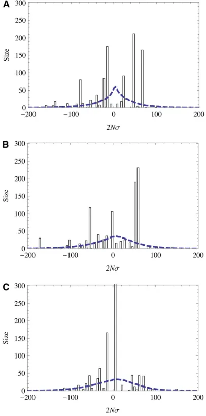
Stationary adaptation in our minimal fitness seascape is characterized by ongoing selection flips, which occur with rate g per site and generate an excess of beneficial over deleterious substitutions, with rates V(s) . V(2s) (see Equation 5). Figure 3A shows the selection-dependent
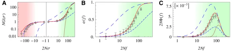
fixation probability G(s) in a linked genome undergoing stationary adaptive evolution. The emergent neutrality re-gimeðjsj,s~Þ, the adaptive regimeðs.~sÞ, and the deleteri-ous passenger regimeðs,2s~Þare marked by color shading. The self-consistent solution of our model (Figure 3A, red line) is in good quantitative agreement with simulation results for a population of linked sequences (Figure 3A, open circles; simulation details are given in section 6 ofFile S1). Data and model show large deviations from single-site the-ory (Figure 3A, long-dashed blue line), which demonstrate strong interference effects in the dense-sweep regime. Fig-ure 3A also shows an effective single-site probability with a globally reduced efficacy of selection,G0ðs=2N~sÞ
(short-dashed blue line). As discussed above, a global reduction in selection efficacy fails to capture the adaptive regime, where mutations have a fixation probability approaching the single-site value 2s.
The crossover between adaptive and emergent-neutrality regimes implies a nonmonotonic dependence of the sub-stitution rate V(s) on the population size: in sufficiently small populations sizes (wheres~,s), beneficial mutations of strengthsare likely to be driver mutations. Hence,V(s) is an increasing function ofNwith the asymptotic behavior VðsÞ≃mNsfamiliar for unlinked sites. In larger populations (wheres~.s), the same mutations are likely to be passenger mutations and V(s) decreases with N toward the neutral rate V(s) ≃ m. The maximal substitution rate is expected to be observed in populations where s~ is similar to s. By the same argument, deleterious mutations have a minimum in their substitution rate in populations where s~ is similar to |s|.
Furthermore, it is instructive to compare our results for stationary adaptation with the classical clonal interference model (Gerrish and Lenski 1998) (see section 5 of File S1 for details). This model focuses exclusively on negative in-terference between strongly beneficial mutations, the case shown in Figure 2F. The resulting approximation for the
fixation probability,GGL(s) =VGL(s)/U(s), is shown in
Fig-ure 3A (brown line). It captFig-ures two salient featFig-ures of the stationary adaptive process: the behavior of strongly
negative interference. Furthermore, mutation-based models with rate and effect of beneficial mutations as input param-eters cannot predict the degree of adaptation, as discussed in section 7.3 ofFile S1.
An important feature of the adaptive dynamics under linkage is the relative weight of driver and passenger mutations in selective sweeps. The fixation probability is highest for strongly beneficial mutationsðs?~sÞ, which are predominantly driver mutations. Nevertheless, the majority of observed substitutions can be moderately adaptive or deleterious passenger mutations (in the process of Figure 3, for example, 60% of all substitutions are passengers, 20% of which are deleterious). The distribution of mutation rates, U(s), and the distribution of fixation rates, V(s) = Vdrive(s) +Vpass(s), are shown in Figure S3 inFile S1.
In Figure 3, B and C, we plot the selection-dependent degree of adaptationa(f) and thefitnessfluxF(f) at statio-narity, which are proportional to each other according to Equation 6. Simulation results are again in good agreement with our self-consistent theory, but they are not captured by single-site theory, single-site theory with globally reduced selection efficacy, or Gerrish–Lenski theory. The functions
a(f) and F(f) display the emergent neutrality regime ðf,s~Þand the adaptive selection regimeðf.~sÞfor genomic sites, which are again marked by color shading. Using Equa-tions 8 and 14, we can obtain approximate expressions for both regimes. Consistent with near-neutral substitution rates, sites in the emergent neutrality regime have a low degree of adaptation andfitnessflux:
aðfÞ ¼ FðfÞ fgLrðfÞ ≃
1 ð1þg=mÞ
f
2~s: (16)
Hence,fixed sites in this regime have nearly random alleles: they cannot carry genetic information. Two processes contribute to this degradation: negative interference slows down the adaptive response to changes in selection, and hitchhiking in selective sweeps increases the rate of delete-rious substitutions. By contrast, sites in the adaptive regime
(f.s~) have a high degree of adaptation and generate most of thefitnessflux. Sites under moderate selection (f≳s~) are still partially degraded by interference, and the negative component of fitnessflux (i.e., the contribution from dele-terious substitutions) is peaked in this regime (see Figure S4 inFile S1). Strongly selected sites (f?~s) are approximately independent of interference. Hence, their degree of adapta-tion andfitnessflux increase to values characteristic of un-linked sites,
aðfÞ ¼ FðfÞ fgLrðfÞ≃
f
fþg=ðmNÞ: (17)
In addition to the selection-dependent quantities dis-cussed so far, our theory also predicts how genome-wide characteristics of the adaptive process depend on its input parameters. The adaptively evolving genome is parameter-ized by the mutation ratem, by the effective population size N, and by three parameters specific to our genomic model: average strengthf and flip rate g of selection coefficients, and genome length L. As an example, Figure 4 shows the dependence of the average degree of adaptationaongand on L, with all other parameters kept fixed (recall that according to Equation 9, this also determines the behavior of the totalfitnessflux,F¼afgL). The genome-wide rate of selectionflips,gL, describes the rate at which new opportu-nities for adaptive substitutions arise at genomic sites. With increasing supply of opportunities for adaption, interference interactions become stronger. This leads to an increase in the neutrality threshold ~s, a decrease in the degree of ad-aptationa, and a sublinear increase of thefitnessfluxF. All of these effects are quantitatively reproduced by the self-consistent solution of our model. As shown in Figure 4, low values of the degree of adaptation aare observed over large regions of the evolutionary parameters gandL. This indicates that a substantial part of the genome can be de-graded to a nearly random state, implying that interference effects can compromise biological functions (seeDiscussion).
Figure 3 Selection regimes of stationary adaptation. (A) Selec-tion-dependentfixation probabil-ity of mutationsG(s), scaled by the population size N. Analytic model solution (red line) and sim-ulation results (circles) show three regimes of selection: (i) ef-fective neutrality regime (white background), where G(s) takes values similar to thefixation probability of independent sites with reduced selection,G0ðs=2N~sÞ(short-dashed blue line); (ii) adaptive regime (green),
whereG(s) crosses over to thefixation probability for unlinked sites with full selection,G0(s) (long-dashed blue line) [the strong-selection part of this
crossover is captured by the Gerrish–Lenski model,GGL(s) (brown line, see section 5 ofFile S1); and (iii) strongly deleterious passenger regime (red),
whereG(s) is exponentially suppressed, but drastically larger than for unlinked sites (long-dashed blue line) due to hitchhiking in selective sweeps. (B and C) Selection-dependent degree of adaptationa(f) andfitnessfluxF(f), scaled byN. Analytical model solution (red line) and simulation results (circles) show two regimes of selection: (i) effective neutrality regime (white background), wherea(f) andF(f) take values similar to those of unlinked sites with reduced selection (short-dashed blue line), and (ii) adaptive regime (green), wherea(f) andF(s) cross over to values of unlinked sites with full selection (short-dashed blue lines). The strong-selection part of the crossover forFis captured by the Gerrish–Lenski model,FGL(f) (brown line, see
Approach to equilibrium in afitness landscape
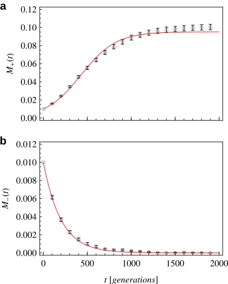
A particular nonstationary adaptive process is the approach to evolutionary equilibrium in a static fitness landscape, starting from a poorly adapted initial genome state. Here, we analyze this mode in our minimal additivefitness model. We choose an initial state at time t= 0 from the family of stationary states presented in the previous section (which is characterized by a valueginitial.0). We study the
evolu-tion of this state for t.0 toward equilibrium under time-independent selection (g = 0; see section 4 of File S1for details of the numerical protocol). Unlike for stationary ad-aptation, the observed dynamics now depend on the initial state. Figure 5 shows the selection-dependent degree of ad-aptationa(f) of this process at three consecutive times. The self-consistent solution of our model is again in good agree-ment with simulation data. There is still a clear grading of genomic sites into an emergent neutrality regime and an adaptive regime, which is again marked by color shading. The neutrality thresholds~ðtÞis now a decreasing function of time. Figure 5 also shows the time derivative of the degree of adaptation, which equals half the adaptive substitution
rate per site:daðfÞ=dt¼ ½VðfÞ2Vð2fÞ=2rðfÞby Equations 4 and 6. Data and model solution show that the adaptive pro-cess is nonuniform: at a given timet, adaptation is peaked at sites of effect fs~ðtÞ, while sites with stronger selection have already adapted at earlier times and sites with weaker selection are delayed by interference. Thus, our model pre-dicts a nonmonotonic behavior of the adaptive rateda(f)/dt on time: for sites with a given selection coefficientf, this rate has a maximum at some intermediate time when s~ðtÞ ¼f, after interference effects have weakened and before these sites have reached equilibrium. This result mirrors the max-imum of the substitution rate V(s) at some intermediate population size for stationary adaptation. As before, a sub-stantial fraction of substitutions are passengers in selective sweeps.
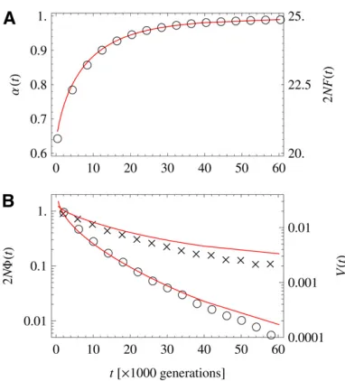
Figure 6A shows the evolution of the genome-averaged degree of adaptation,a, and of the mean populationfitness, F, which are linearly related by Equation 1. Thefitnessflux
F = dF/dt and the total substitution rate V are plotted in Figure 6B. According to Equation 4, these quantities are
Figure 4 Degree of adaptation at stationarity. Results from our model (red lines), simulation results (circles), and values for independent sites (dashed blue lines) of the degree of adaptation are plotted (A) against the total selectionflip rategLfor two different values of the genome length,
L ¼ 200 (circles) andL ¼ 2000 (diamonds), and (B) against the total genomic mutation ratemNLfor two different values of the selectionflip rate, 2Ng¼0.01 (circles) and 2Ng¼0.1 (triangles). Note that for the smaller value ofg, the time to reach stationarity is very long, which limits the numerical results to smaller values of the system size. Other system parameters areN¼4000, 2Nm¼0.025, and2Nf550, and simulation time is 8·105generations.
Figure 5 Selection regimes for approach to equilibrium. The population evolves from a poorly adapted initial state to a high-fitness equilibrium state. The degree of adaptation (circles and solid line) and its time de-rivative (which is related to the adaptive rate per site, crosses and dashed line) are shown for three consecutive times,t= 600, 8000, and 55,000 generations. Theory lines are obtained by numerically solving Equation 6. The emergent neutrality regimeðs,s~Þand the adaptive regimeðs.s~Þ
linked in a time-dependent way,FðtÞ ¼VðtÞs~ðtÞ VðtÞ~sðtÞ. We observe thatfitness increases monotonically with time. Its rate of increase F rapidly slows down as the system comes closer to evolutionary equilibrium, whereas the total substitution rateVshows a slower approach to equilibrium. A qualitatively similar time dependence offitness and sub-stitution rate has been reported in a long-term bacterial evolution experiment by Barricket al.(2009).
Discussion
Interference can dominate genetic drift
Interference interactions in the dense-sweep regime may be complicated in their details, but their net effect is simple: genomic sites with selection coefficients s smaller than a threshold~shave nearly randomfixed alleles, and mutations at these sitesfix with near-neutral rates. The neutrality thresh-olds~ is given by the total rate of selective sweeps, Vdrive, as
shown in Equation 15. Emergent neutral mutations, as well as more deleterious changes, fix as passengers in selective sweeps. That is, both classes of mutations are subject to in-terference, not genetic drift, as a dominant stochastic force. The resultingfixation ratesV(s) depend only weakly on the effective population size N. Mutations with larger beneficial effectðs.s~Þsuffer gradually weaker interference interactions. Hence, theirfixation rates show a drastic increase toward the Haldane–Kimura valueV(s) = 2mNsset by genetic drift.
At a qualitative level, these results tell the story of the Hill–Robertson effect: genetic linkage reduces the efficacy of selection. Quantitatively, they demonstrate that emergent
neutrality is not equivalent to a simple reduction in effective population size. The fixation rate of emergent neutral and deleterious passenger mutations can heuristically be inter-preted as a linear reduction in effective population size by a factor 2N~s, but this approximation breaks down for muta-tions with larger beneficial effect; see Equation 14 and Fig-ure 3A. In other words, we cannot absorb the effects of interference into a single modified strength of genetic drift. Of course, both interference and genetic drift are stochastic processes that randomize alleles of genomic sites. However, they have fundamentally different characteristics: genetic drift is a diffusion process causing independent changes in allele frequencies in each generation, whereas interference generatescoherentchanges over time intervals given by the inverse selection coefficient of the driver mutation.
Fluctuations and intermittency of the adaptive process
Given genetic drift and interference as stochastic driving forces, how stochastic are the resulting adaptive substitution dynamics? This question has been addressed in several recent studies, which treat the adaptive process as a traveling
fitness wave (Rouzineet al.2003, 2008; Desai et al.2007; Hallatschek 2011). If all mutations are assumed to have the same effect, these models are solvable. Onefinds a traveling wave with a deterministic bulk of stationary shape (given by a mutation–selectionflux state) and a stochastic tip. The variance of this wave determines its speed (i.e., thefitness
flux) by Fisher’s fundamental theorem. Given a stationary bulk of the wave, thefitnessflux has only smallfluctuations around its mean value. However, the recent solvable model of Hallatschek (2011) contains largefluctuations in popula-tion size, which may be related tofluctuations infitnessflux. The adaptive process studied in this article shows a drastically different behavior. In our model,fitness effects at genomic sites follow a distributionr(f) with shape parame-ter k. For the case of exponential r(f) (given by k= 1), a snapshot of the population’sfitness distribution at a given point in time is shown in Figure 7A. This distribution has large shapefluctuations throughout its bulk, not just at the tip. It shows that the adaptive process is dominated byfew co-occurring beneficial mutations of large effect, whereas a stationary wave is maintained by many mutations of smaller effect. As a consequence, the fitnessflux becomes intermit-tent: on small timescales, it has largefluctuations around its mean value, as shown in Figure 7A. Movies of the intermit-tentfitness wave are available; see Figure 8. Importantly, this strong stochasticity accelerates evolution: at given rate Ub
and mean effectsb¼ ð1=UbÞ
RN
0 sUðsÞdsof beneficial
muta-tions, our model produces a much higher mean fitness flux than the traveling-wave solution. The reason is simple: a dis-tribution of selection coefficients generates dynamics domi-nated by strong driver mutations, whose effect is substantially larger than the mean (Parket al.2010).
How relevant is this mode of intermittent adaptation for actual populations? We expect our model to be applicable to microbial laboratory populations, which often fall into the
range of evolutionary parameters considered by this study. For example, the population- and genome-wide mutation rate in anEscherichia colipopulation of sizeN= 105ismNL
= 250 (Drake et al. 1998). Our simulations cover system sizes up to mNL = 2000; large populations are simulated by scaling up m while keeping mNL constant (for details, see section 6 ofFile S1).
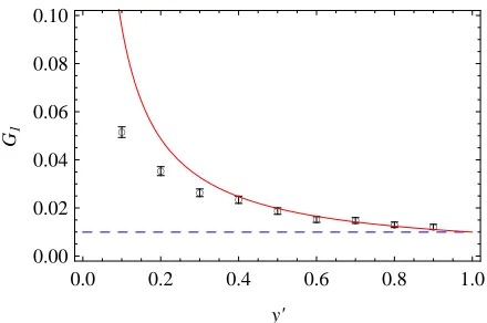
To further test the range of applicability of our model, we evaluate the stochasticity of the fitness flux for different
Figure 7 Stochasticity of the adaptive process. The speed of adaptation and the shape of the distribution offitnesses in the population are gov-erned by largefluctuations. (A) Snapshot of thefitness distribution in the population, centered around the meanfitness. The shape of this distri-bution is very different from the average shape, shown as a dashed line. The dynamics are governed by fewfitness classes with a large number of individuals (note the logarithmic axis). The evolution of this distribution is shown in three movies; see Figure 8. (B) Time series of the cumulativefitness fluxFDt(t), which is defined as the net selective effect of all allele frequency
changesDxi(i= 1,. . .,L) within a short time intervalDt(Mustonen and Lässig
2010): FDtðtÞ ¼PLi¼1ðDxiÞ@Fðx1ðtÞ; . . . ;xLðtÞ; tÞ=@xi (we useDt = 20 generations). This flux is intermittent;i.e., the traveling fitness wave has short-term boosts in its speed. (C) Stochasticity of thefitnessflux. The ratio of variance and meanfitnessfluxFDt(t) over a population’s history is plotted
as a function of the total mutation ratemNLfor selection shape parameters
k=1
2(circles),k= 1 (squares), andk= 2 (triangles). For a given total mutation
rate, the stochasticity is highest fork=1
2and decreases with increasingk.
However, the stochasticity remains approximately constant for increasing system size. Other simulation parameters areN= 500 (a and b),N= 1000 (c),L= 500, 2Ng= 0.1, 2Ng= 0.025,k= 1, and2Nf¼50.
Figure 8 Intermittentfitness waves. The three videos show the distribu-tion of genotypefitness values in a population, as it changes over time in a dense-sweep adaptive process. The meanfitness is kept to 0 by nor-malization. Thefitness distribution is strongly stochastic: at any specific time, its shape is very different from the long-time average shape (plotted as a dashed line). There are recurrent selective sweeps: a new high-fitness genotype appears in the right-hand tail of the distribution, gains frequency, and moves quickly toward the center. Simulations are shown for three different distributionsr(f) of genomic selection coefficients, characterized by the shape parameterk. (a)k= 0.5 (stretched exponential tail). This case has the strongest stochasticity in the shape of thefitness wave, because exceptionally strong sweeps are generated with significant probability. (b)
k= 1 (exponential tail). (c)k= 2 (Gaussian tail). This case shows a smoother evolution of the fitness wave, which results from average-strength sweeps generated at a more regular pace. Other simulation parameters areN= 1000,L= 1000, 2Nm= 0.025, 2Ng= 0.1, and2Nf ¼50. (A) Movie 1: http://www.genetics.org/content/suppl/2011/09/16/genetics. 111.132027.DC1/Movie1.mov
(B) Movie 2: http://www.genetics.org/content/suppl/2011/09/16/genetics. 111.132027.DC1/Movie2.mov
evolutionary parameters. We define the cumulative fitness
fluxFDt(t) as the selective effect of allele frequency changes over a short time intervalDt(we useDt= 20 generations), and we evaluate the ratioeof variance and mean ofFDt(t) over a population’s history (Mustonen and Lässig 2010). In Figure 7C, we plot this ratio as a function of the genome length L for fitness effect distributions r(f) of different shapes, which have a stretched exponential (k = 1
2), an
exponential (k = 1), or a Gaussian (k = 2) tail for large values off. Movies of the fitness wave are available for all three cases; see Figure 8. As expected, we observe a decrease in stochasticity with increasing shape parameter k. This is consistent with a crossover tofitness waves with deterministic bulk shape in the limit of a sharp distribution (k / N). However, we do not see any evidence of a crossover to de-terministic fitness waves with increasing genome length L: the stochasticity ratioestays roughly constant and thefitness wave retains strong shape fluctuations even for the largest values of L. At the same time, our model predictions of the
fixation probabilityG(s) overestimate the simulation results at large L, in particular for strongly beneficial driver muta-tions. This may indicate a crossover to a new mode of adap-tive evolution: selecadap-tive sweeps are driven cooperaadap-tively by multiple beneficial mutations, but the adaptive dynamics re-main intermittent. This regime is not yet covered by any analytical scheme, but we expect that our interaction calculus can be extended to more complex multidriver sweeps.
Passenger mutations and the inference of selection
Our model predicts an important consequence of interference interactions: a substantial fraction of the genomic substitu-tions observed in laboratory or field data of dense-sweep processes are not driver mutations, but moderately beneficial or deleterious passenger mutationsfixed by hitchhiking. This fraction increases with increasing population size N or ge-nome lengthL. Disentangling driver and passenger mutations in the dense-sweep regime poses a challenge for the inference of selection from such data. This problem arises not only for asexual populations, but also for linked genome segments of recombining genomes (Fay 2011). The general rationale of this article applies to recombining populations as well, if we replace the total genome length by the linkage correlation length. Adaptation under linkage confounds the standard population-genetic inference of selection based on the statis-tics of polymorphisms and substitutions, because it reduces the statistical differences between weakly and strongly se-lected genomic changes. To develop selection inference meth-ods applicable under strong interference, we have to extend our picture of the genome state to polymorphism spectra. This will be the subject of a future study.
Viability limits of evolution under linkage
To summarize, we have shown that interference can strongly reduce the degree of adaptation of an evolving population and hence its viability. This result is likely to be valid beyond the specifics of our model: in any ongoing
adaptive process driven by time-dependent selection, a large reduction in the speed of adaptation due to interference is inextricably linked to a large fitness cost compared to unlinked sites. However, genome states with a large fraction of effectively randomized sites are not a plausible scenario for microbial evolution, where a substantial degree of adaptation is maintained and dysfunctional parts are expected to be pruned from the genome. This suggests that natural populations limit genome degradation by interfer-ence. Microbial experiments and genomic analysis may help us to better understand how.
Acknowledgments
This work was supported by Deutsche Forschungsgemein-schaft grant SFB 680 and grant GSC 260 (Bonn Cologne Graduate School for Physics and Astronomy). V.M. acknowl-edges the Wellcome Trust for support under grant 091747. This research was also supported in part by the National Science Foundation (NSF) under grant NSF PHY05-51164 during a visit at the Kavli Institute of Theoretical Physics (Santa Barbara, CA).
Literature Cited
Andolfatto, P., 2007 Hitchhiking effects of recurrent beneficial amino acid substitutions in the Drosophila melanogaster ge-nome. Genome Res. 17(12): 1755–1762.
Bachtrog, D., and I. Gordo, 2004 Adaptive evolution of asexual populations under Muller’s ratchet. Evolution 58(7): 1403–1413. Barrick, J. E., D. S. Yu, S. H. Yoon, H. Jeong, T. K. Oh et al., 2009 Genome evolution and adaptation in a long-term exper-iment with Escherichia coli. Nature 461(7268): 1243–1247. Barton, N. H., 1995 Linkage and the limits to natural selection.
Genetics 140: 821–841.
Barton, N. H., 2000 Genetic hitchhiking. Philos. Trans. R. Soc. Lond. B Biol. Sci. 355(1403): 1553–1562.
Betancourt, A. J., 2009 Genomewide patterns of substitution in adaptively evolving populations of the RNA bacteriophage ms2. Genetics 181: 1535–1544.
Bush, R. M., C. A. Bender, K. Subbarao, N. J. Cox, and W. M. Fitch, 1999 Predicting the evolution of human influenza A. Science 286(5446): 1921–1925.
Charlesworth, B., 1994 The effect of background selection against deleterious mutations on weakly selected, linked variants. Genet. Res. 63(3): 213–227.
Charlesworth, B., 1996 Background selection and patterns of ge-netic diversity in Drosophila melanogaster. Genet. Res. 68(2): 131–149.
Charlesworth, B., M. T. Morgan, and D. Charlesworth, 1993 The effect of deleterious mutations on neutral molecular variation. Genetics 134: 1289–1303.
Comeron, J. M., and M. Kreitman, 2002 Population, evolutionary and genomic consequences of interference selection. Genetics 161: 389–410.
Comeron, J. M., A. Williford, and R. M. Kliman, 2008 The Hill-Robertson effect: evolutionary consequences of weak selection and linkage infinite populations. Heredity 100(1): 19–31. de Visser, J., C. W. Zeyl, P. J. Gerrish, J. L. Blanchard, and R. E.
de Visser, J. A. G. M., and D. E. Rozen, 2006 Clonal interference and the periodic selection of new beneficial mutations in Escher-ichia coli. Genetics 172: 2093–2100.
Desai, M. M., and D. S. Fisher, 2007 Beneficial mutation selection balance and the effect of linkage on positive selection. Genetics 176: 1759–1798.
Desai, M. M., D. S. Fisher, and A. W. Murray, 2007 The speed of evolution and maintenance of variation in asexual populations. Curr. Biol. 17(5): 385–394.
Drake, J. W., B. Charlesworth, D. Charlesworth, and J. F. Crow, 1998 Rates of spontaneous mutation. Genetics 148: 1667–1686. Eyre-Walker, A., and P. D. Keightley, 2007 The distribution of fitness effects of new mutations. Nat. Rev. Genet. 8(8): 610–618. Fay, J. C., 2011 Weighing the evidence for adaptation at the
mo-lecular level. Trends Genet 27: 343–349.
Felsenstein, J., 1974 The evolutionary advantage of recombina-tion. Genetics 78: 737–756.
Fisher, R., 1930 The Genetical Theory of Natural Selection. Claren-don Press, Oxford.
Fogle, C. A., J. L. Nagle, and M. M. Desai, 2008 Clonal interfer-ence, multiple mutations and adaptation in large asexual pop-ulations. Genetics 180: 2163–2173.
Gerrish, P. J., and R. E. Lenski, 1998 The fate of competing ben-eficial mutations in an asexual population. Genetica 102–103 (1–6): 127–144.
Gillespie, J., 1984 Molecular evolution over the mutational land-scape. Evolution 38(5): 1116–1129.
Gillespie, J. H., 2001 Is the population size of a species relevant to its evolution? Evolution 55(11): 2161–2169.
Haldane, J., 1937 The effect of variation offitness. Am. Nat. 71 (735): 337–349.
Haldane, J., 1957 The cost of natural selection. J. Genet. 55: 511–524. Hallatschek, O., 2011 From the cover: the noisy edge of traveling
waves. Proc. Natl. Acad. Sci. USA 108(5): 1783–1787. Hermisson, J., and P. S. Pennings, 2005 Soft sweeps: molecular
population genetics of adaptation from standing genetic varia-tion. Genetics 169: 2335–2352.
Hill, W., and A. Robertson, 1966 The effect of linkage on limits to artificial selection. Genet. Res. 8: 269–294.
Imhof, M., and C. Schlotterer, 2001 Fitness effects of advanta-geous mutations in evolving Escherichia coli populations. Proc. Natl. Acad. Sci. USA 98(3): 1113–1117.
Kaiser, V. B., and B. Charlesworth, 2009 The effects of deleterious mutations on evolution in non-recombining genomes. Trends Genet. 25(1): 9–12.
Kao, K., and G. Sherlock, 2008 Molecular characterization of clonal interference during adaptive evolution in asexual popu-lations of Saccharomyces cerevisiae. Nat. Genet. 40(12): 1499– 1504.
Kassen, R., and T. Bataillon, 2006 Distribution offitness effects among beneficial mutations before selection in experimental populations of bacteria. Nat. Genet. 38(4): 484–488.
Kim, Y., and W. Stephan, 2000 Joint effects of genetic hitchhiking and background selection on neutral variation. Genetics 155: 1415–1427.
Kim, Y., and W. Stephan, 2003 Selective sweeps in the pres-ence of interferpres-ence among partially linked loci. Genetics 164: 389–398.
Kimura, M., 1962 On the probability offixation of mutant genes in a population. Genetics 47: 713–719.
Kinnersley, M. A., W. E. Holben, and F. Rosenzweig, 2009 E unibus plurum: genomic analysis of an experimentally evolved polymorphism in Escherichia coli. PLoS Genet. 5(11): e1000713.
MacLean, R. C., and A. Buckling, 2009 The distribution offitness effects of beneficial mutations in Pseudomonas aeruginosa. PLoS Genet. 5(3): e1000406.
Martin, G., and T. Lenormand, 2006 A general multivariate ex-tension of Fisher’s geometrical model and the distribution of mutationfitness effects across species. Evolution 60(5): 893–907. McVean, G., and B. Charlesworth, 2000 The effects of Hill-Robertson interference between weakly selected mutations on patterns of molecular evolution and variation. Genetics 155: 929–944. Muller, H., 1932 Some genetic aspects of sex. Am. Nat. 66(703):
118–138.
Muller, H., 1950 Our load of mutations. Am. J. Hum. Genet. 2(2): 111–176.
Mustonen, V., and M. Lässig, 2007 Adaptations tofluctuating selec-tion in Drosophila. Proc. Natl. Acad. Sci. USA 104(7): 2277–2282. Mustonen, V., and M. Lässig, 2008 Molecular evolution under
fitnessfluctuations. Phys. Rev. Lett. 100(10): 108101.
Mustonen, V., and M. Lässig, 2009 From fitness landscapes to seascapes: non-equilibrium dynamics of selection and adapta-tion. Trends Genet. 25(3): 111–119.
Mustonen, V., and M. Lässig, 2010 Fitness flux and ubiquity of adaptive evolution. Proc. Natl. Acad. Sci. USA 107(9): 4248–4253. Neher, R. A., and T. Leitner, 2010 Recombination rate and selec-tion strength in HIV intra-patient evoluselec-tion. PLoS Comput. Biol. 6(1): e1000660.
Orr, H. A., 2000 The rate of adaptation in asexuals. Genetics 155: 961–968.
Orr, H. A., 2003 The distribution offitness effects among benefi -cial mutations. Genetics 163: 1519–1526.
Park, S.-C., and J. Krug, 2007 Clonal interference in large popu-lations. Proc. Natl. Acad. Sci. USA 104(46): 18135–18140. Park, S.-C., D. Simon, and J. Krug, 2010 The speed of evolution in
large asexual populations. J. Stat. Phys. 138(1–3): 381–410. Perfeito, L., L. Fernandes, C. Mota, and I. Gordo, 2007 Adaptive
mutations in bacteria: high rate and small effects. Science 317 (5839): 813–815.
Rambaut, A., O. G. Pybus, M. I. Nelson, C. Viboud, J. K. Tauben-bergeret al., 2008 The genomic and epidemiological dynamics of human influenza A virus. Nature 453(7195): 615–619. Rokyta, D. R., P. Joyce, S. B. Caudle, and H. A. Wichman, 2005 An
empirical test of the mutational landscape model of adaptation using a single-stranded DNA virus. Nat. Genet. 37(4): 441–444. Rouzine, I. M., J. Wakeley, and J. Coffin, 2003 The solitary wave of asexual evolution. Proc. Natl. Acad. Sci. USA 100(2): 587–592. Rouzine, I. M., E. Brunet, and C. O. Wilke, 2008 The traveling-wave approach to asexual evolution: Muller’s ratchet and speed of adaptation. Theor. Popul. Biol. 73(1): 24–46.
Rozen, D. E., J. A. G. M. de Visser, and P. J. Gerrish, 2002 Fitness effects of fixed beneficial mutations in microbial populations. Curr. Biol. 12(12): 1040–1045.
Silander, O. K., O. Tenaillon, and L. Chao, 2007 Understanding the evolutionary fate offinite populations: the dynamics of mu-tational effects. PLoS Biol. 5(4): e94.
Smith, J. M., 1971 What use is sex? J. Theor. Biol. 30(2): 319–335. Smith, J. M., 1976 What determines the rate of evolution? Am.
Nat. 110(973): 331–338.
Smith, J. M., and J. Haigh, 1974 The hitch-hiking effect of a fa-vourable gene. Genet. Res. 23(1): 23–35.
Tenaillon, O., O. K. Silander, J.-P. Uzan, and L. Chao, 2007 Quantifying organismal complexity using a population genetic approach. PLoS ONE 2(2): e217.
Waxman, D., 2007 Mean curvaturevs.normality: a comparison of two approximations of Fisher’s geometrical model. Theor. Popul. Biol. 71(1): 30–36.
Wilke, C. O., 2004 The speed of adaptation in large asexual pop-ulations. Genetics 167: 2045–2053.
Appendix
Fixation Probability Under Interference Interactions
Here we compute the conditional fixation probability G(s,t | s9,t9), of a target mutation with selection coeffi -cientsand origination timet, which is subject to an inter-fering mutation with selection coefficients9and origination time t9, for the different cases of Figure 2: interference by deleterious background mutations (t9 ,tands9 , 2|s|, Figure 2, A and B), beneficial background mutations (t9 ,t
and s9 . |s|, Figure 2, C and D), and beneficial future mutations (t9 . t and s9 . |s|, Figure 2, E and F). We neglect the effects of interference mutations weaker than the target mutations (2|s|,s9 ,|s|), which is consis-tent with the hierarchy approximation. We also neglect the effects of deleterious future mutations, which are small (if a deleterious mutation arises after the target mutation, this deleterious mutation cannot preventfixation of the target mutation). Without interference, a target mutation of frequency x0 has a fixation probability
G0ðx0;sÞ ¼ ð12e22Nsx0Þ=ð12e22NsÞ, which is determined
by selection and genetic drift. In contrast, we treat beneficial interfering mutations as destined for fixation; that is, we assume they have overcome genetic drift.
Interference by deleterious background mutations
The diagrams in Figure 2, A and B, describe background selection caused by strongly deleterious alleles originat-ing before the target mutation. Case a occurs with proba-bility x9Q(x9, s), where x9 is the frequency of the interfering mutation at time tand Q(x9,s) is the proba-bility distribution of this frequency. This case results in likely loss of the target mutation, because the interfering mutation has a selection coefficient stronger in magnitude than the target mutation. Case b occurs with probability (1 2x9)Q(x9, s), and its dominant effect is to boost the initial frequencyx0of the target mutation by a factor 1/(1 2x9) (see section 1 ofFile S1for a numerical validation). The resulting conditionalfixation probability of the target mutation is
Gðs;tjs9;t9Þ ¼
Z1
0
dx9Qðx9 ;sÞð12x9ÞG0 1 Nð12x9Þ; s
:
(A1)
Because the interfering mutation is deleterious, its probability distributionQ(x9;s) is dominated by very small frequencies x9 > 1. For s $ 0 and x9 > 1, the fixation probability G0(x0,s) is in good approximation linear in its first argument. In that case, the factor (12x9) cancels out and we recover the unlinked fixation probability Gðs;tjs9;t9Þ ¼G0ð1=N;sÞ. This argument does not apply
to deleterious target mutations, but they can be neglected because G0(x0, s) is exponentially small for s , 0, even
including a boost in the initial frequency.
Interference by beneficial background mutations
The diagrams of Figure 2, C and D, describe positive and negative interference by a selective sweep starting at timet9 ,t. Case d occurs with probability 12x9and results in likely loss of the target mutation. Case c occurs with prob-ability x9 and boosts the initial frequency x0 of the target
mutation by a factor 1/x9(see Figure S1 inFile S1). Treating the interfering mutation as deterministic, its frequencyx9at time t is given by x9¼xdetðt2t9; s9Þ ¼1=½1þ ðN21Þ
expð2s9ðt2t9ÞÞ. Hence, we obtain
Gðs;tjs9;t9Þ ¼
Z1
0
dx9 dðx9 2xdetðt2t9;s9ÞÞx9G0 1 Nx9;s
;
(A2)
wheredis Dirac’s delta distribution.
Interference by future beneficial mutations
The diagrams in Figure 2, E and F, describe positive and negative interference by a selective sweep starting at time
t9 .t. Case e occurs with probability xG0(x,t9 2t;x0,s)
and results in likelyfixation of the target mutation by hitch-hiking. Here,G0(x,t9 2t;x0,s)is the probability that a
tar-get mutation of initial frequency x0 at time t has reached
frequencyxat timet9withoutinterference in between. Case f occurs with probability (1 2 x)G0(x, t9 2 t; x0, s) and
results in likely loss of the target mutation. Hence, we obtain
Gðs;tjs9;t9Þ ¼R10dx x G0ðx;t9 2t;x0;sÞ
¼
G0ðx0;sÞ=1þe2^sðt92tÞG0ðx0;sÞx20121
ðfors.0Þ; x0es^ðt92tÞ þ12e^sðt92tÞG0ðx0;sÞ ðfors,0Þ; (A3)
see section 2 ofFile S1for the evaluation of this integral in the diffusion approximation. The regularized selection co-efficients^ is a shorthand for the crossover from strong to weak selection:s^≃sforNs≳1 ands^≃1=2NforNs≲1.
Interference by past and future sweeps
First, we compute the conditional fixation probability G(s,t|s9,t9,s99,t99) of a target mutation subject to inter-ference by the closest background sweep (with parameters
t9 , t and s9 . s) and the closest future sweep (with parameterst99 . tands99 .s). As shown above, the net positive contributions to this probability arise from partial hitchhiking with the past sweep and subsequent full hitch-hiking with the future sweep; see Figure 2, C and E. Com-bining Equations A2 and A3, we obtain
Gðs;tjs9;t9;s99;t99Þ ¼Z1 0
dx9Z1
0
dx dðx9 2xdetðt2t9;s9ÞÞx9xG0 x;t99 2t; 1
Nx9; s
:
(A4)
between the sweeps themselves are neglected (such as rescue of the target mutation by a future sweep, following negative interference by a past sweep). This is in tune with our self-consistent determination of the sweep rate, which absorbs the overlap exclusion between driver mutations [i.e., the conditiont99 2t9 .tfix(s9)] into a reduced
uni-form or “mean-field”rate Vdrive(s) given by Equations 11
and 12. In this approximation, a target mutation of selection coefficientsis subject to interference by stronger selective sweeps at a total rateV.ðsÞ ¼RNsds9Vdriveðs9Þ:We can now
integrate Equation A4 over past and future sweeps (i.e., driver mutations) with an exponential distribution of wait-ing timest2t9andt99 2t,
GðsÞ¼
Zt
2Ndt9
ZN t
dt99 ZN
s
ds9 ZN
s
ds99Vdriveðs9ÞVdriveðs99Þe2V.ðsÞðt992t9ÞGðs;tjs9;t9;s99;t99Þ:
(A5)
Using Equation A3, the integrations overs99 andt99can be treated analytically, and we obtain
GðsÞ ¼Rt2Ndt9RNjsjds9Vdrive
s9e2V.ðjsjÞðt2t9ÞR1 0dx9d
x92xdet
t2t9;s9
· (
x9G0 1 Nx9;s
2F1
1; V.ðsÞs^; 1þV.ðsÞ^s; 12Nx9G0 1 Nx9;s
ðfors.0Þ;
1
Nðjs^j þV.ðjs^jÞÞ Nx9G0 1 Nx9; s
js^j þV.ðjsjÞ
ðfors,0Þ;
(A6)
where 2F1(a, b, c; z) is a hypergeometric function. The
remaining integrals in this expression can be evaluated nu-merically in a straightforward way (see section 4 ofFile S1 for an iterative procedure). Neglecting the (numerically smaller) integral over past sweeps, we obtain a closed form of Equation A6,
GðsÞ ¼
8 > < > :
G0 1 N;s
2F1
1;V.ðsÞ^s; 1þV.ðsÞs^; 12NG0 1 N; s
ðfors.0Þ;
1
Nðj^sj þV.ðj^sjÞÞ NG0
1
N; s
js^j þV.ðjsjÞ
ðfors,0Þ: (A7)
These results also determine the fixation probability of passenger mutations in the decomposition of Equation 13,
GpassðsÞ ¼Gð
sÞ2pdriveðsÞG0ðsÞ 12pdriveðsÞ ;
(A8)
where Pdrive(s) is given by Equation 12 and G0ðsÞ ¼ ð12exp½22sÞ=ð12exp½22NsÞ. The neutrality thresholds~
is obtained by Taylor expansion of Equation A7; we obtain GðsÞ ¼ ð1=NÞ þs=½1þ2NV.ðsÞ þ Oðs2Þ. Comparing with the corresponding expansion of G0(s) shows that linkage
GENETICS
Supporting Information
http://www.genetics.org/content/suppl/2011/09/16/genetics.111.132027.DC1
Emergent Neutrality in Adaptive Asexual Evolution
Stephan Schiffels, Gergely J. Szöll}osi, Ville Mustonen, and Michael Lässig