FULL PAPER
Application of a simplified calculation
for full-wave microtremor
H
/
V
spectral ratio
based on the diffuse field approximation
to identify underground velocity structures
Hao Wu
1*, Kazuaki Masaki
2, Kojiro Irikura
2and Francisco José Sánchez‑Sesma
3Abstract
Under the diffuse field approximation, the full‑wave (FW) microtremor H/V spectral ratio (H/V) is modeled as the square root of the ratio of the sum of imaginary parts of the Green’s function of the horizontal components to that of the vertical one. For a given layered medium, the FW H/V can be well approximated with only surface waves (SW) H/V of the “cap‑layered” medium which consists of the given layered medium and a new larger velocity half‑space (cap layer) at large depth. Because the contribution of surface waves can be simply obtained by the residue theorem, the computation of SW H/V of cap‑layered medium is faster than that of FW H/V evaluated by discrete wavenumber method and contour integration method. The simplified computation of SW H/V was then applied to identify the underground velocity structures at six KiK‑net strong‑motion stations. The inverted underground velocity structures were used to evaluate FW H/Vs which were consistent with the SW H/Vs of corresponding cap‑layered media. The previous study on surface waves H/Vs proposed with the distributed surface sources assumption and a fixed Rayleigh‑ to‑Love waves amplitude ratio for horizontal motions showed a good agreement with the SW H/Vs of our study. The consistency between observed and theoretical spectral ratios, such as the earthquake motions of H/V spectral ratio and spectral ratio of horizontal motions between surface and bottom of borehole, indicated that the underground velocity structures identified from SW H/V of cap‑layered medium were well resolved by the new method.
Keywords: Diffuse field approximation, Microtremor H/V spectral ratio, Full‑wave, Surface waves, Underground velocity structures
© The Author(s) 2017. This article is distributed under the terms of the Creative Commons Attribution 4.0 International License (http://creativecommons.org/licenses/by/4.0/), which permits unrestricted use, distribution, and reproduction in any medium, provided you give appropriate credit to the original author(s) and the source, provide a link to the Creative Commons license, and indicate if changes were made.
Open Access
*Correspondence: [email protected]
1 Earthquake Engineering Group, Geo‑Research Institute, 2‑1‑2, Otemae,
Chuo‑ku, Osaka, Japan
Full list of author information is available at the end of the article
Introduction
The microtremor H/V spectral ratio (H/V) is the most pop-ular approach to estimate the predominant period of a site (Nakamura 1989, 2000; Lermo and Chávez-García 1993). In what has been controversial, Nakamura (1989, 2000) proposed to consider this ratio to be the empirical transfer function. Using a numerical simulation, Lachet and Bard (1994) verified that the natural period of the sedimentary site coincides well with the predominant period of H/V.
These issues have raised an assortment of opinions on the characteristics and origin of features of H/V, i.e., predomi-nant period and amplitude, being a SH waves transfer func-tion (Nakamura 1989, 2000; Lermo and Chávez-García
1993), the role of ellipticity of fundamental mode or high modes of Rayleigh waves and the emergency of Airy phase of Love waves (Lachet and Bard 1994; Konno and Ohmachi
and Love waves). Accordingly, various methods to identify underground velocity structures have been proposed for three-component station measurements, depending on different assumptions on the origin, e.g., ellipticity of fun-damental mode of Rayleigh waves (Fäh et al. 2001), higher modes of surface waves (Arai and Tokimatsu 2004), or SH-wave transfer function (Lin et al. 2014).
Since microtremor consists of both body and surface waves, a full-wave description is desirable to interpret the
H/V. Diffuse field approximation is one of the promising theories to accomplish it. The diffuse field concept origi-nated in acoustics and was firmly established for elasticity by Weaver (1982). But the roots of the idea can be traced back to the pioneering work of Aki (1957) who used ambi-ent seismic noise (ASN) in the SPAC method (for spa-tial autocorrelation). The short-range cross-correlations of noise in a small array and its azimuthal average allow, through the argument of the Bessel function of zero order, to retrieve the phase velocity of Rayleigh waves. Aki’s pio-neering work addressed first ideas and issues that were later formalized by Weaver (1982) as diffuse fields. The connection with 2D elasticity was pointed out by Sánchez-Sesma and Campillo (2006). It has been proposed that the coda of earthquakes can be seen as a realization of a dif-fuse field (Shapiro et al. 2000; Hennino et al. 2001; Mar-gerin 2009). In several instances, the ASN allows Green’s function retrieval from the average of cross-correlation between two receivers within a diffuse seismic field. Sha-piro and Campillo (2004), Sabra et al. (2005), and Shapiro et al. (2005) confirmed that ASN is generally diffuse. We assert that the key of this fact lies in multiple scattering. The properties and the conditions of emergence of a dif-fuse field have been explored by many researchers world-wide (e.g., Weaver and Lobkis 2001; Sánchez-Sesma and Campillo 2006; Sánchez-Sesma et al. 2008). For the appli-cations, the diffuse field assumption allows to get useful approximations of the Green’s Function from cross-cor-relation of recorded motions. Even Mulargia (2012) who claims that ASN is not diffuse accepts that it holds signifi-cant imaging properties. Based on the diffuse field approx-imation, the directional energy density is proportional to the imaginary part of the Green’s function when source and receiver coincide with each other both in position and direction (Sánchez-Sesma et al. 2008). The FW H/V is then expressed as the square root of the sum of imaginary parts of the horizontal components of Green’s function to that of the vertical counterpart (Sánchez-Sesma et al. 2011). In the diffuse field description, the imaginary part of the Green’s function incorporates naturally the contributions of both body (BW) and surface waves (SW). Therefore, an explanation on the origin of H/V is achieved by full-wave.
Lontsi et al. (2015) used the FW description to invert
H/V recorded and processed from different depths to
identify underground velocity structures at a couple of sites in Germany. They used a straightforward calcula-tion inspired on the convencalcula-tional discrete wavenumber method to evaluate the Green’s functions. This full-wave approach is time consuming and limits the application of inversion of FW H/V to some extent. García-Jerez et al. (2013) evaluated the imaginary parts of the Green’s func-tions, accounting for the separate contributions of body and surface waves using the Cauchy’s contour integration method, for which the computation of surface waves cor-responding to residues is fast. They further developed two faster codes for inversion of both the FW H/V and joint inversion, adding the velocity dispersion curve of funda-mental mode of Rayleigh waves, and then implemented these codes to identify underground velocity structures at some sites (García-Jerez et al. 2016; Piña-Flores et al.
2017). That has been a major accomplishment, but the computation of body waves which contribute little to the full-wave consumes most of the computing time. Also, the efficiency of their code (opened to public) for for-ward calculation of FW H/V reduces significantly, when the number of frequencies of H/V is larger than 1000 and the number of layers is more than 5. To circumvent those drawbacks, we explore other ways in which we see room for improvement. Harvey (1981) applied the locked-mode approximation method to approximate the Green’s func-tions in time domain for full-wave with superposition of normal modes (surface waves) by adding a large veloc-ity half-space to the bottom of given velocveloc-ity structures. He referred to this large velocity half-space as “cap layer.” Because the computation of surface waves is quite fast and the computation of body waves is not needed, the computational efficiency is better than the one achieved with other methods, such as reflectivity, Thomson– Haskell propagation matrix, and global matrix, all within the discrete wavenumber summation scheme.
In this study, we adopt the diffuse field approximation (DFA) and investigate the applicability of the cap-layered medium to compute the H/V from the surface waves of that waveguide. Our approach allows identifying the underground velocity structures between the surface and bottom of boreholes at six KiK-net stations where the PS logging data are not reliable enough to explain the observed H/Vs. In the framework of SW H/V, we inves-tigate the differences between SW H/V of our approach and SW H/V of the previous study on microtremor H/V
spectral ratio developed by Arai and Tokimatsu (2004). We finally discuss the validity of identified underground velocity structures by comparing observed results with theoretical results, such as earthquake motions H/V
Formula of microtremor H/V spectral ratio based on diffuse field approximation
Based on the diffuse field approximation, the FW H/V is expressed as follows:
where ImG is the imaginary part of the Green’s function when both source and receiver coincide with each other both in position and direction (Sánchez-Sesma et al.
2011), and the subscripts 11 and 22 mean two horizontal components, and 33 the vertical one. The imaginary part of the Green’s functions “detects” energies that are both radiated from and coming back to the source. Im G11, Im
G22, and Im G33 are proportional to directional energy densities associated with the three degrees of freedom. Other components, such as G12 (or G21), G13 (or G31), and G23 (or G32), are not needed, and the imaginary parts of them are zero for coincident source and receiver. The right side of Eq. (1) only depends on the underground velocity structure, such as density, P- and S-wave velocity, and thickness of each layer, regardless of sources distri-bution and proportion of body and surface waves, which makes it the signature of the site. The corresponding code (Sánchez-Sesma et al. 2011) was inspired on the discrete wavenumber method to carry out the integrations in the wavenumber domain.
García-Jerez et al. (2013) proposed to evaluate the Green’s functions by the Cauchy’s contour integra-tion method, because the Green’s funcintegra-tions for surface waves can be quickly evaluated as the sum of residues. For horizontally layered media, the imaginary part of the Green’s functions and the SW H/V is expressed as follows:
where AR and AL are the medium responses of Rayleigh and Love waves, respectively (Harkrider 1964), u/w is the ellipticity of Rayleigh waves, m and n are the order of modes for Rayleigh and Love waves, M and N are the largest order of higher modes for Rayleigh and Love waves. Because the medium responses of higher modes,
(1)
e.g., larger than the fifth mode, are much smaller than those of fundamental mode and only contribute in a short period range, without loss of generality, M and N
are set to be 5 in the following calculations. Regarding the calculation of surface waves, the ellipticity, the medium response terms AR of Rayleigh waves, and AL of Love waves should be evaluated from the fundamental to the fifth higher mode, and for a given layered medium, Saito
and Kabasawa (1993) proposed the “compound matrix”
to overcome the numerical instability at high frequen-cies of the Thomson–Haskell propagation matrix. We improved their code and enabled it to evaluate Eq. (4). For a layered medium consisting of less than 10 layers, the computation of SW H/V by our code on a desktop computer (64-bit, Windows 8.1, Intel Core i7, 3.20 GHz, RAM 8.0 GB) takes no more than 1 s even if the num-ber of frequencies reaches 2000. It is significantly faster than the computation of FW H/V by discrete wavenum-ber method (Sánchez-Sesma et al. 2011) which usually takes several or tens of minutes. It is also faster than the MATLAB runtime environment developed by García-Jerez et al. (2016) based on contour integration method which for the same problem takes several or tens of sec-onds. Furthermore, the numerical instability that can be observed at high frequencies of certain higher modes of Rayleigh waves for the García-Jerez et al. (2016)’s code is avoided.
Approximation of FW H/V for two‑layered medium
Harvey (1981) proposed that by adding a large velocity cap layer to a given layered medium and fixing the bot-tom, the Green’s function of full-wave could be approxi-mated with superposition of normal modes of surface waves. However, the effects of (1) depth of the upper interface, (2) the largeness of velocity of the cap layer, and (3) the impedance ratios of target layered medium, on the applicability of this approximation, were not discussed. In this section, we add a large velocity cap layer at large depth to examine the feasibility of approximation of the Green’s function of full-wave with the Green’s function of surface waves. This consideration is implicitly involved in the study of Arai and Tokimatsu (2004) who added two thick layers with large velocity to reach the engineering bedrock. They only formulated the H/V of surface waves based on distributed surface sources assumption.
much less sensitivity than S-wave velocity to H/V (e.g., Arai and Tokimatsu 2004; Lontsi et al. 2015). We regard this layered medium as “target” two-layered medium, and the layered medium composed of target layered medium and a cap layer as “cap-layered” medium.
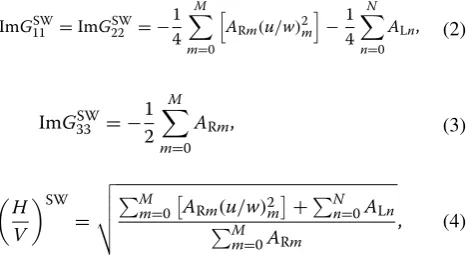
First, we investigate the effect of depth of upper inter-face of cap layer on the applicability of approximating the FW H/V of target two-layered medium with SW H/V of cap-layered medium. Table 2 lists the parameters of cap-layered media with three different depths (i.e., 2.5, 5, and 10 times the wavelength λ0 at fundamental frequency or period) of upper interface of cap layers. For target two-layered medium, λ0 is just four times the thickness of first layer, whatever the velocity and frequency is. The veloc-ity of the cap layer is fixed, twice as large of the layer
above the cap layer. As shown in the left panel of Fig. 1, the SW H/V of the target two-layered medium is almost the same as FW H/V in the period smaller than the pre-dominant period of fundamental S-wave resonance mode-Tp0, namely 0.4 s, according to one quarter wave-length law. This indicates that the contribution of full-wave in the short period range is nearly the same as that of surface waves in the first layer. As shown in the mid-dle panel of Fig. 1, the SW H/V of cap-layered medium approximates well to the FW H/V of target two-layered medium in the period ranging from 0.1Tp0 to 5Tp0 of the target medium if the depth of the upper cap layer is larger than 5λ0. The reason is that the large velocity cap layer in the deep converts the body waves that are leaked from the first layer of target two-layered medium into higher modes of surface waves. It is obvious from Fig. 2 that the largest peak of SW H/V of target two-layered medium is caused by a local trough in the vertical component which corresponds to the cutoff of vertical medium response of the first higher mode of Rayleigh waves. The cutoff of horizontal medium response has little effect on the larg-est peak, because its amplitude is not only smaller than that of fundamental mode of Rayleigh waves, but much smaller than that of Love waves. Due to the addition of cap layer, the vertical medium responses of the second, third and fourth higher modes of Rayleigh waves just fill in the local trough caused by the first higher mode, and this leads to a good approximation of FW H/V of tar-get two-layered medium with SW H/V of cap-layered medium. Therefore, although the main advantage of SW H/V is its computation efficiency over FW H/V, the calculation of medium responses of surface waves gives Table 1 Target two‑layered medium (Vp = 2Vs, den‑
sity = 2.0 g/cm3)
Layer Vs Depth
1 Vs1= 100 m/s 10 m(=λ0/4)
2 Vs2= 3Vs1 ∞
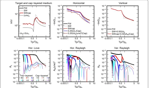
Table 2 Cap‑layered media with different depths of the upper interface of cap layer (Vp= 2Vs, density = 2.0 g/cm3)
Layer Vs Depth
1 Vs1= 100 m/s 10 m(=λ0/4)
2 Vs2= 3Vs1 100 m(= 2.5λ0) 200 m(= 5λ0) 400 m(= 10λ0) Cap 2Vs2 ∞
10−1
100
101
H/V
0.05 0.1 0.5 1 5 10 Tp/Tp0
Target layered medium
FW(target) SW (u/w)0
Vs2=3Vs1
10−1
100
101
H/V
0.05 0.1 0.5 1 5 10 Tp/Tp0
Depth effect
FW(target) SW(Dep.=2.5λ0)
SW(Dep.=5λ0)
SW(Dep.=10λ0)
Vs2=3Vs1; VsCap=2Vs2
10−1
100
101
H/V
0.05 0.1 0.5 1 5 10 Tp/Tp0
VsCap effect
FW(target) SW(VsCap=1.2Vs2) SW(VsCap=1.5Vs2)
SW(VsCap=4.5Vs2)
Vs2=3Vs1; Depth=10λ0
insight into the different contribution from fundamental and higher modes of both Rayleigh and Love waves.
Second, we investigate the effect of the cap layer veloc-ity on the feasibilveloc-ity of approximating the FW H/V of target two-layered medium with SW H/V of cap-layered medium. Table 3 lists the parameters of cap-layered media with different velocities of the cap-layer. The depth of upper interface of cap layer is set as 10λ0 (i.e., 400 m here). As shown in the right panel of Fig. 1, the SW H/V
of cap-layered medium agrees well with the FW H/V of target two-layered medium if the velocity of cap layer is larger than 1.5 times the velocity of the second layer (Vs2). It is considered that the small velocity of cap layer (e.g., 1.2Vs2) is not enough for totally converting the body waves into surface waves.
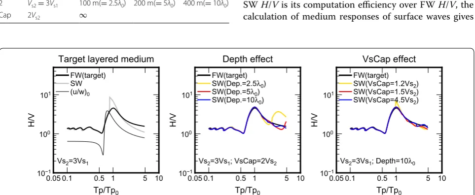
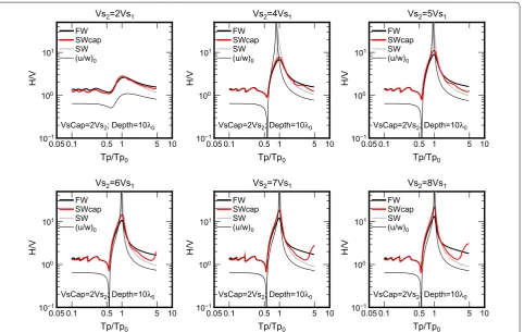
Third, we investigate the effect of the impedance ratio of two-layered medium on the feasibility of approximat-ing the FW H/V of target two-layered medium with SW
H/V of cap-layered medium. Table 4 lists the parameters of target two-layered media with different impedance ratios. The depth of upper interface of cap layer is set to be 10λ0, and the velocity of cap layer of these target two-layered media is twice as large of Vs2. Figure 3 shows that the amplitudes of FW and SW H/Vs increase with the impedance ratio. This fact prompted Nakamura to con-sider H/V as a transfer function. Obviously, the imped-ance ratio is relevant. Ellipticity of the fundamental mode of Rayleigh waves is different from FW H/V, not only the amplitude but also the predominant period. For the Rayleigh’s fundamental mode, the conspicuous period of
10−1
Target and cap−layered medium
10−12
ellipticity coincides with the well-known local minimum in the vertical component. It is gradually close to that of FW H/V as the impedance ratio increases. This fact was carefully studied in numerical simulations (Bonne-foy-Claudet et al. 2008). Similarly, for the SW H/V, the predominant periods of SW H/Vs of two-layered media for which the peaks coincide with the troughs of higher mode or fundamental mode (if the impedance ratio is large) of Rayleigh waves in the vertical component vary with impedance ratio. Figure 3 also shows that when the impedance ratio is not larger than 6, the SW H/V of cap-layered medium agrees well with the FW H/V of two-lay-ered medium in the period range, e.g., 0.1Tp0–5Tp0, even if only the contributions from fundamental to the fifth higher modes of surface waves are included in the SW
H/V. Nolet et al. (1989) concluded that the evaluation of the Green’s function requires 50–100 higher modes for locked-mode approximation. The site they selected is rather hard because the Vs in the first layer is as large as 1500 m/s. In contrast, the sites in our study are much softer, e.g., the Vs is about 300 m/s in the first layer and is smaller than 1000 m/s from the surface downward to 100 m in depth. This suggests that the Nolet et al. (1989)’s study was barely related with the results presented herein. The amplitudes of tiny fluctuations at very short periods, e.g., below 0.1Tp0, for SW H/V are slightly smaller than for FW H/V due to the loss of modes higher than 5 for the target two-layered media. This small discrepancy between SW and FW H/Vs is difficult to detect for realis-tic multilayered media, such as those sites studied by Arai and Tokimatsu (2004) and Lunedei and Albarello (2009). Considering the temporal variation of microtremors, this small discrepancy seems negligible, e.g., smaller than one standard deviation of observed H/V, which we discuss
later for one site. Besides, it only affects the accuracy of uppermost velocity structures (e.g., thinner than 1 m) which is far from engineering interest. The amplitude of SW H/V is twice as large as that of FW H/V around the predominant period so that the difference cannot be neglected if the impedance ratio is larger than 6.
Figure 4 shows the comparison between FW H/V of target two-layered medium (Vs2 = 8Vs1) and SW H/V of cap-layered medium for which the depth of upper inter-face of cap layer is 10λ0 (i.e., 400 m), as well as the imagi-nary parts of the Green’s functions and vertical medium responses from fundamental to the fifth higher modes. Due to cutoff effect of higher modes, the vertical medium responses from modes higher than third have no contri-butions at periods longer than the predominant period. Therefore, summation of higher modes larger than the fifth cannot improve the approximation of FW H/V of target two-layered medium with SW H/V of cap-layered medium at periods longer than the predominant period. We further place the cap layer at a great depth, such as 100λ0 (i.e., 4000 m here) to investigate whether the SW
H/V of cap-layered medium can approximates well with FW H/V. Figure 5 shows the comparison between FW
H/V of target two-layered medium (Vs2 = 8Vs1) and SW
H/V of cap-layered medium for which the depth of upper interface of cap layer is as large as 100λ0, as well as the imaginary parts of the Green’s functions and vertical medium responses from fundamental to the 25th higher modes of Rayleigh waves. The discrepancy between FW H/V of target medium and SW H/V of cap-layered medium around the predominant period still cannot be neglected, as the vertical medium responses of higher modes of Rayleigh waves do not totally fill in the trough caused by the vertical medium response of fundamen-tal mode. Therefore, even if the cap layer is located at a great depth and more modes are considered, the FW H/V
of target medium with large impedance ratio cannot be well approximated with SW H/V of cap-layered medium. Tokimatsu and Tamura (1995) pointed out that if the impedance ratio is too large, the contribution of body waves is much larger than that of surface waves near the predominant period. It is thus considered that the cap layer fails to totally convert body waves into surface waves in this case. Applying rigid boundary condition Table 3 Cap‑layered media with different velocities in the
cap layer (Vp= 2Vs, density = 2.0 g/cm3)
Layer Vs Depth
1 Vs1= 100 m/s 10 m(=λ0/4) 2 Vs2= 3Vs1 400 m(= 10λ0) Cap 1.2Vs2 1.5Vs2 4.5Vs2 ∞
Table 4 Two‑layered media with different impedance ratios and cap‑layered media (Vp= 2Vs, density = 2.0 g/cm3)
a The thickness of second layer is infinite for two-layered medium
Layer Vs Depth
1 Vs1= 100 m/s 10 m(=λ0/4)
10−1
100
101
H/V
0.05 0.1 0.5 1 5 10 Tp/Tp0
Vs2=2Vs1 FW
SWcap SW (u/w)0
VsCap=2Vs2; Depth=10λ0
10−1
100
101
H/V
0.05 0.1 0.5 1 5 10 Tp/Tp0
Vs2=4Vs1 FW
SWcap SW (u/w)0
VsCap=2Vs2; Depth=10λ0
10−1
100
101
H/V
0.05 0.1 0.5 1 5 10 Tp/Tp0
Vs2=5Vs1 FW
SWcap SW (u/w)0
VsCap=2Vs2; Depth=10λ0
10−1
100
101
H/
V
0.05 0.1 0.5 1 5 10 Tp/Tp0
Vs2=6Vs1 FW
SWcap SW (u/w)0
VsCap=2Vs2; Depth=10λ0
10−1
100
101
H/
V
0.05 0.1 0.5 1 5 10 Tp/Tp0
Vs2=7Vs1 FW
SWcap SW (u/w)0
VsCap=2Vs2; Depth=10λ0
10−1
100
101
H/
V
0.05 0.1 0.5 1 5 10 Tp/Tp0
Vs2=8Vs1 FW
SWcap SW (u/w)0
VsCap=2Vs2; Depth=10λ0
Fig. 3 Comparison between FW H/Vs (thick black), SW H/Vs (gray), ellipticity of fundamental mode of Rayleigh waves (thin black) of two‑layered media with six different impedance ratios, and SW H/Vs (red) of corresponding cap‑layered media (in all cases VsCap= 2Vs2, Depth = 10λ0). As for the two‑layered media, Vs2= 2Vs1 in the upper left panel, Vs2= 4Vs1 in the upper middle panel, Vs2= 5Vs1 in the upper right panel, Vs2= 6Vs1 in the lower left panel, Vs2= 7Vs1 in the lower middle panel and Vs2= 8Vs1 in the lower right panel
10−1
100
101
H/
V
0.05 0.1 0.2 0.5 1 5 10 Tp/Tp0
Depth=10λ0
10−12
10−11
10−10
10−9
10−8
10−7
10−6
10−5
10−4
−ImG
33
0.05 0.1 0.2 0.5 1 5 10 Tp/Tp0
Vertical
10−12
10−11
10−10
10−9
10−8
10−7
10−6
10−5
10−4
AR
0.05 0.1 0.2 0.5 1 5 10 Tp/Tp0
Ver. Rayleigh(Cap) M=N=5
FW SWcap
Vs2=8Vs1; VsCap=2Vs2
FW
SWcap=0.5ΣAR(Cap)
0 1 2 3 4 5
(Margerin 2009) at the upper interface of cap layer is considered an effective solution to totally convert body waves into surface waves.
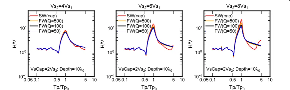
Another aspect that is of interest in practice is the effect of damping ratio or quality factor-Q which is used in the calculation of FW H/V but not included in SW H/V. In the FW H/V, some damping was introduced by adding a small imaginary part to frequency and also using some material damping. Although the purpose was mainly to stabilize the results and to smooth the integrands in the wavenumber domain (Sánchez-Sesma et al. 2011), the practical interest of damping in realistic soil configura-tions led us to explore the effects of small material damp-ing usdamp-ing a quality factor-Q. This is not accounted for in the theory, but in some cases adding small amount of
damping allows for results closer to observations (e.g., Lawrence and Prieto 2011). We explore the effects of quality factor-Q on FW H/Vs of two-layered media with three different impedance ratios shown in Fig. 6. It sug-gests that the difference of FW H/Vs caused by three dif-ferent Q values (50, 100 and 500) is negligible. Thus, the
discrepancy between FW H/V of target medium with
large impedance ratio and SW H/V cannot be attributed to the damping ratio or Q values.
Finally, it should be noted that the large velocity cap layer at large depth is just an artificial layer used to con-vert the body waves leaked from the bottom of given lay-ered medium into surface waves of cap-laylay-ered medium.
Meanwhile, the SW H/V of cap-layered medium is
regarded a simplified calculation of FW H/V of layered
10−1
100
101
H/V
0.05 0.1 0.2 0.5 1 5 10 Tp/Tp0
Depth=100λ0
10−12
10−11
10−10
10−9
10−8
10−7
10−6
10−5
10−4
−ImG
33
0.05 0.1 0.2 0.5 1 5 10 Tp/Tp0
Vertical
10−12
10−11
10−10
10−9
10−8
10−7
10−6
10−5
10−4
AR
0.05 0.1 0.2 0.5 1 5 10 Tp/Tp0
Ver. Rayleigh(Cap) M=N=25
FW SWcap
Vs2=8Vs1; VsCap=2Vs2 FWSWcap=0.5ΣAR(Cap)
0 1 5 10 20 25
Fig. 5 H/Vs, imaginary parts of the Green’s function in the vertical component and vertical medium responses of Rayleigh waves from fundamental mode to 25th higher mode. The depth of upper interface of cap layer is 100λ0. Left: FW H/V (thick black) for target two‑layered medium (Vs2= 8Vs1), and SW H/V (red) for cap‑layered medium (VsCap= 2Vs2, Depth = 100λ0). Middle: imaginary parts of the Green’s function of FW (thick black) in the vertical component for target two‑layered medium and that of SW (red) for cap‑layered medium. Right: vertical medium responses of Rayleigh waves for fundamental mode (black), first higher mode (red), fifth higher mode (blue), 10th higher mode (cyan), 20th higher mode (thin black), and 25th higher mode (purple). For clarity, medium responses are depicted for only six modes. The medium responses below 0.2Tp0 are omitted because the calculation becomes rather difficult when the dispersion curves of higher modes are quite close to one another at very short periods
10−1
100
101
H/V
0.05 0.1 0.5 1 5 10 Tp/Tp0
Vs2=4Vs1 SW(cap) FW(Q=500) FW(Q=100) FW(Q=50)
VsCap=2Vs2; Depth=10λ0
10−1
100
101
H/V
0.05 0.1 0.5 1 5 10 Tp/Tp0
Vs2=6Vs1 SW(cap) FW(Q=500) FW(Q=100) FW(Q=50)
VsCap=2Vs2; Depth=10λ0
10−1
100
101
H/V
0.05 0.1 0.5 1 5 10 Tp/Tp0
Vs2=8Vs1 SW(cap) FW(Q=500) FW(Q=100) FW(Q=50)
VsCap=2Vs2; Depth=10λ0
medium, and we agree that microtremor consists of full-wave, but not surface waves only. Based on the afore-mentioned discussions, we conclude that the FW H/V of target layered medium should be well approximated with SW H/V of cap-layered medium in the period range, e.g., 0.1Tp0–5Tp0, under the following conditions: The imped-ance ratio of target layered medium is not larger than 6, and the S-wave velocity of cap layer is about twice as large as that in the half-space of target layered medium, the depth of upper interface of cap layer is about (5–10)λ0. However, it should be noted that Q = 100 might be too large for FW H/V at soft sediment sites, and thus further investigation is needed.
Approximation of FW H/V for multilayered medium
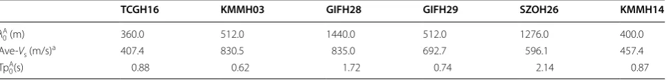
In Japan, PS logging data between surface and bottom of boreholes at most KiK-net strong-motion stations are available, so the underground velocity structures of PS logging data are adopted to generate multilayered media. With respect to the corresponding cap-layered media, we set the velocity of the cap layer as about two times larger than that in the above layer. Because one cannot pre-cisely estimate the Tp0 or λ0 for a given layered medium, we define the “apparent” predominant period of S-wave fundamental mode (Tp0A) as the ratio of the “apparent” wavelength of fundamental mode (λ0A) for the given lay-ered medium to the thickness-weighted average S-wave velocity (Fäh et al. 2001). The “apparent” wavelength of fundamental mode (λ0A) is four times the depth from sur-face to the uppermost intersur-face of half-space, but not four times the thickness of first layer anymore. Both Tp0A and λ0A become the “real” Tp0 and λ0 for the two-layered medium (single layer over a half-space) and tend to be the “real” ones if the velocity contrast at the interface of half-space is large enough for multilayered medium. We find that if the depth of cap layer is set to be about (5–10)
λ0A, the SW H/V of cap-layered medium approximates well to the FW H/V of target multilayered medium. Six KiK-net stations were selected after a careful scru-tiny that accounts for local geology, seismicity, and site effects. They do not locate near the edge between basin and mountain nor close to active faults so that the 3D effects are considered minor. Figure 7 shows the S-wave
velocity profiles in the top panels at six KiK-net stations. Table 5 lists the basic parameters, such as Tp0A, thickness-averaged Vs, and λ0A for velocity profiles at these stations. The numerical values show the Tp0A at the interface of half-space of target layered medium in black and that at the uppermost interface of cap layer in red. It is obvious that the cap layer at large depth produces a Tp0A about 5–10 times as larger as that for target layered medium. These 1D vertical profiles are obtained from PS logging data. In most circumstances, that 1D profile is verified by studying the measured amplification from an earth-quake, such as comparing the observed surface/bottom of borehole spectral ratio with theoretical 1D transfer function (e.g., Thompson et al. 2012). Another approach is to use microtremor to accomplish such verification by comparing the observed microtremor H/V with the the-oretical H/V, considering that the soil models are 1D or only depth dependent at these stations. The underground velocity structures consisting of PS logging data are used to evaluate four theoretical H/Vs in the bottom panels, i.e., ellipticity of fundamental mode of Rayleigh waves, FW H/V and SW H/V of the multilayered medium, and SW H/V of the corresponding cap-layered medium. The coincidence between FW and SW H/Vs of multilayered media in the short period range at all stations again indi-cates that the contribution of surface waves which are trapped in the shallow layers is overwhelmingly domi-nant. By just adding a cap layer to the bottom of bore-hole, the SW H/Vs of cap-layered media approximate the FW H/Vs well at almost all the stations except KMMH14 at which a relatively large impedance ratio near the bot-tom of borehole could be responsible for the discrepancy between FW H/V of multilayered medium and SW H/V
of cap-layered medium. However, this discrepancy is negligible given that the microtremor is subjected to the temporal variance (Okada 2003).
The ellipticities of fundamental mode of Rayleigh waves at all stations have two peaks which are caused by the underground velocity structures of shallow layers, and deep layers, respectively. The sharp peak at periods shorter than 0.5 s at TCGH16 station corresponds to the large impedance ratio in the shallow layers as shown in the S-wave velocity profiles. The sharp peaks at periods
(See figure on next page.)
longer than 0.5 s at other stations correspond to the large impedance ratio in the deep layers near the bottom of boreholes. Both peaks of ellipticity of fundamental mode of Rayleigh waves at GIFH28 are moderate. This is attrib-uted to the moderate impedance ratio from surface to bottom of borehole.
The observed microtremor H/Vs at six KiK-net stations are also shown in bottom panels of Fig. 7. We conduct the microtremor measurement with a three-component velocity seismometer, a GPS receiver, and a recorder with 24 bits. We conduct the measurement for 30–60 min with 100 Hz sampling at all stations except TCGH16 where we observed as long as 12 h. We remove those time windows (Tw = 40.96 s) including extremely large ampli-tude which is caused by nearby human activities, such as jogging, vehicles, before obtaining the power spec-tra in three components. These power specspec-tra in three components are then averaged over the number of time windows. The observed H/V is obtained from the square ratio of average power spectra in the horizontal compo-nents (arithmetic summation of north–south (NS) and east–west (EW) components) to that in the vertical com-ponent, just as proposed by Arai and Tokimatsu (2004) and numerically verified by Albarello and Lunedei (2013). Smoothing with b = 50 by Konno and Ohmachi (1998) is finally implemented on the observed H/V. Thus only one
H/V without temporal variability can be obtained at one site. As the record is long at TCGH16, we divide it into 24 parts each of which is used to evaluate H/V to inves-tigate the temporal variation of observed H/V. We take the average H/V as the observed one at TCGH16 and find the standard deviation at each period. The average H/V is shown in thick black curve, and the ones obtained from the average plus and minus one standard deviation are shown in dashed curves in Fig. 7. Temporal variation can be observed, yet it is very small. The mismatch between the FW H/V and observed H/V suggests that the under-ground velocity structures of PS logging data are not fully reliable and thus should be improved through inversion of H/V.
Identification of underground velocity structures from SW H/V
Since the computation of medium responses of sur-face waves is significantly faster than the computation of full-wave, and FW H/V can be approximated with SW H/V
by just adding a cap layer to the bottom of given layered medium, we prefer to identify the underground velocity structures from SW H/V. We perform the identification by simulated annealing algorithm which is elaborated in Satoh (2006). Generally, this algorithm finds many local minima at the beginning and gradually converges to a global minimum. The temperature scheme is expressed as Tk = T0∙exp(− ckα),
where k is the step of cooling, Tk is the temperature at the kth step, T0 is the initial temperature, and c and α are key parameters controlling the cooling speed. We set T0, c, and
α to be 1.0, 1.0, and 0.6, respectively, iterations at one step to be 5, and total steps 1000. The objective function Em is
defined as follows: (Saguchi et al. 2009)
where (H/V)fSW denotes the SW H/V of cap-layered
medium, (H/V)fobs denotes the observed H/V, f denotes
fre-quency (equally spaced precisely as it is in FFT), fmin and
fmax denote the minimum and maximum frequencies of
the target fitting frequency range, respectively. The fmin is determined in consideration of the depth of underground velocity structures from surface to bottom, e.g, it may be not deep enough to explain peak at low frequency or long period. The fmax is the Nyquist frequency—50 Hz, if sam-pling frequency is 100 Hz, whereas fmax = 20 Hz is better for some sites. In this study, we set fmin to be 0.25–0.5 Hz, and fmax to be 20–50 Hz. The weight function is usually employed in the objective function to guarantee a good fit-ting over a broad frequency range. Typically, the expressions for the objective or cost functions are weighted sums of residuals. The choice of the weights is a matter of taste. Cer-tainly, a common selection aimed to smooth out the results is to use frequency so that larger frequencies with their mul-tiple oscillations have less constraining power. Our previous studies (Wu et al. 2012, 2016; Wang et al. 2017) suggested that the linear “frequency” worked well as the weight func-tion, while Satoh (2006) suggested a logarithmic frequency to be another weight function. The temporal variation of observed H/V is considered small, and it is not included in the objective function. The discussion about the effect of different weight functions on the objective function and how to incorporate the temporal variation in the objective function is important, yet beyond the scope of this study.
If there is not any a priori knowledge about the under-ground velocity structures, the identified velocity struc-tures are not unique by inversion of H/V only. It is a good practice to implement the joint inversion of both H/V
and dispersive curve, such as Parolai et al. (2005), Picozzi et al. (2005), Arai and Tokimatsu (2005), and Piña-Flores et al. (2017). An alternative method to uniquely identify the underground velocity structures by the inversion of
H/V only is to make use of a priori knowledge. In this study, we refer to the PS logging data to be the initial underground velocity structures rather than those gen-erated by genetic algorithm (Piña-Flores et al. 2017). It
is well known that the accuracy of velocity structures of PS logging data in shallow layers is generally not reliable enough. The velocities of soil layers near the surface in most cases are unstable and fluctuate, and the interface between two adjacent layers is not easy to detect and so is the layer thickness. As shown in Fig. 7, the H/Vs for ini-tial cap-layered media match well with the observed ones at relative long periods, such as around 0.6 s at TCGH16, 0.6 s at KMMH03, 2.0 s at SZOH26, and 0.8 s at KMMH14, respectively. This is attributed to the fact that thickness and average velocity from surface downward to the layer boundary which has a remarkable velocity con-trast at each site is clearly detectable for PS logging data. It implies that the velocity structures in moderate depth accounting for the H/Vs at relative long periods are reli-able. Thus we fix the average velocity down to the moder-ate depth (including the bottom of the boreholes) during the identification. Moreover, considering the density and
Vp are insensitive to H/V, we fix the densities and the Poisson ratios so that Vp can be evaluated from identi-fied Vs. Under these constraints, we are able to uniquely identify the velocity structures in the shallow layers from our SW H/V for cap-layered media. Although there is a trade-off relationship between Vs and thickness, identifi-cation of both Vs and thickness in each layer converges faster than that of only Vs or only thickness in each layer at some stations.
Figure 8 shows all the profiles of identified Vs structures between the surface and bottom of boreholes as well as the initial ones, and the observed and theoretical H/Vs. The initial underground velocity structures are composed of those PS logging data and a cap layer. Additional file 1: Tables A1–A6 list the initial and identified underground
velocity structures at six KiK-net stations, while the PS logging data used to construct the initial underground velocity structures are available online (see “Availabil-ity of data and materials”). The large variance of veloc-ity profiles and corresponding SW H/Vs (shown in light pink) is explained that the simulated annealing algorithm is likely to find many solutions at local minima before the solution converges toward a global minimum. The black numerical values in the left bottom of H/V panels are the objective function Em between observed H/Vs and SW
H/Vs for initial underground velocity structures. The red numerical values in the left bottom of H/V panels are the objective function Em between observed H/Vs and SW
H/Vs for identified underground velocity structures. The smaller Em values suggest that the SW H/Vs for identi-fied underground velocity structures agree better with the observed H/Vs at these stations than SW H/Vs for initial underground velocity structures. Meanwhile, the FW H/Vs, evaluated with identified underground veloc-ity structures without cap layer, are in good agreement with SW H/Vs of corresponding cap-layered media. It in turn suggests that the SW H/V of cap-layered medium can be considered as a simplified calculation of FW H/V
of layered medium without cap layer, to identify the underground velocity structures.
Comparison with previous study on H/V
and validation of identified underground velocity structures
Regarding SW H/V, we studied the differences between
the diffuse field approximation (DFA-SW H/V) and
the Arai and Tokimatsu’s (2004) proposal that consid-ers surface waves from a random distribution of surface Table 5 Basic parameters of velocity profiles at six KiK‑net stations
a Thickness-averaged S-wave velocity
TCGH16 KMMH03 GIFH28 GIFH29 SZOH26 KMMH14
λ0A (m) 360.0 512.0 1440.0 512.0 1276.0 400.0
Ave‑Vs (m/s)a 407.4 830.5 835.0 692.7 596.1 457.4
Tp0A(s) 0.88 0.62 1.72 0.74 2.14 0.87
(See figure on next a page.)
Fig. 8 Profiles of underground velocity structures between the surface and the bottom of boreholes (upper) and H/Vs (lower) at six KiK‑net strong‑ motion stations. In the upper panels, thin black lines show the profiles of initial underground velocity structures, light pink lines show the profiles of underground velocity structures identified during all the iterations, and thick black lines show the profiles of identified underground velocity struc‑ tures. In the lower panels, thick black curves denote the observed H/Vs, thin black curves denote the SW H/Vs of initial cap‑layered media, light pink curves denote the SW H/Vs of all identified cap‑layered media during the iterations, red curves denote the SW H/Vs of identified cap‑layered media, and cyan curves denote the FW H/Vs of identified layered media. The numerical values in black represent the objective function Em between observed H/Vs and SW H/Vs of initial cap‑layered media, and the numerical values in red represent the objective function Em between observed
1
10
100
1000
Depth(m)
100 1000 Vs(m/s) TCGH16cap
10−1 100 101
H/V
0.01 0.1 1 10 Period(sec) Initial
All Identified
Observed
SWcap(Init) SWcap(All) SWcap(Iden) FW(Iden)
0.25 0.11
1
10
100
1000
Depth(m)
100 1000 Vs(m/s) KMMH03cap
10−1 100 101
H/V
0.01 0.1 1 10 Period(sec) Initial
All Identified
Observed
SWcap(Init) SWcap(All) SWcap(Iden) FW(Iden)
0.33 0.14
1
10
100
1000
Depth(m)
100 1000 Vs(m/s) GIFH28cap
10−1 100 101
H/V
0.01 0.1 1 10 Period(sec) Initial
All Identified
Observed
SWcap(Init) SWcap(All) SWcap(Iden) FW(Iden)
0.32 0.12
1
10
100
1000
Depth(m)
100 1000 Vs(m/s) GIFH29cap
10−1 100 101
H/V
0.01 0.1 1 10 Period(sec) Initial
All Identified
Observed
SWcap(Init) SWcap(All) SWcap(Iden) FW(Iden)
0.34 0.09
1
10
100
1000
Depth(m)
100 1000 Vs(m/s) SZOH26cap
10−1 100 101
H/V
0.01 0.1 1 10 Period(sec) Initial
All Identified
Observed
SWcap(Init) SWcap(All) SWcap(Iden) FW(Iden)
0.32 0.17
1
10
100
1000
Depth(m)
100 1000 Vs(m/s) KMMH14cap
10−1 100 101
H/V
0.01 0.1 1 10 Period(sec) Initial
All Identified
Observed
SWcap(Init) SWcap(All) SWcap(Iden) FW(Iden)
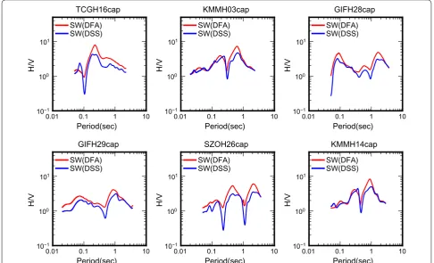
sources (DSS-SW H/V). Figure 9 shows the comparison between (DFA) SW and DSS-SW H/Vs. Just as we did on the observed H/Vs, smoothing with b = 50 by Konno and Ohmachi (1998) is implemented on the DSS-SW H/Vs, but not on (DFA) SW H/Vs as they are already smoothed. Both of these two SW H/Vs at six stations show a quali-tative agreement. It is attributed to the fact that both of these two studies incorporate the contributions of both fundamental and higher modes of surface waves (e.g., the medium response terms of AR and AL), despite of differ-ent premises. On the other hand, the amplitudes of DSS-SW H/Vs at peaks are a bit smaller than those of SW
H/Vs. It agrees with the study of Kawase et al. (2015) who
compared the DSS-SW and FW H/Vs by use of
under-ground velocity structures identified from DSS-SW H/Vs. The constant Rayleigh-to-Love waves amplitude ratio for horizontal motions (R/L) in a period range of 0.1–5 s which is assumed to by Arai and Tokimatsu (2004) sug-gests that the shape of DSS-SW H/V is the same as H/V
evaluated from the medium responses of fundamen-tal and higher modes of Rayleigh waves, and the differ-ent amplitude between them only relies on the value of R/L. In fact, the R/L may vary with site condition, as
reviewed by Bonnefoy-Claudet et al. (2006b). The appar-ent peaks of DSS-SW H/V around 0.07 s at TCGH16 and 0.4 s at KMMH14, and sharp troughs imply the limita-tion of R/L which should be variable with period rather than constant. Arai and Tokimatsu (2004) assumed that the source-to-receiver distance is larger than one wave-length. Thus their DSS-SW H/V involves the power spec-tra of displacements in the horizontal components (G13 and G23) excited by vertical loading force, and the power spectra of displacement in the vertical component (G31 and G32) excited by horizontal loading force. In contrast, the imaginary parts of G13, G23, G31, and G32 which are not required for evaluating FW H/V in Eq. (1) are zero when source and receiver coincide with each other both in position and direction. It is considered another reason for the difference between (DFA) SW and DSS-SW H/Vs. Lunedei and Albarello (2009) followed the assumption of Arai and Tokimatsu (2004) that surface waves were gen-erated by a random distribution of surface sources, and improved the formulation for surface waves approxima-tion by considering the effects of damping and discarding the R/L assumption. They further released the limitation on the source-to-receiver distance (e.g., r = 0) to develop
10−1
100
101
H/V
Period(sec) TCGH16cap SW(DFA) SW(DSS)
10−1
100
101
H/V
Period(sec) KMMH03cap SW(DFA) SW(DSS)
10−1
100
101
H/V
Period(sec) GIFH28cap SW(DFA) SW(DSS)
10−1
100
101
H/
V
Period(sec) GIFH29cap SW(DFA) SW(DSS)
10−1
100
101
H/
V
Period(sec) SZOH26cap SW(DFA) SW(DSS)
10−1
100
101
H/
V
0.01 0.1 1 10 0.01 0.1 1 10 0.01 0.1 1 10
0.01 0.1 1 10 0.01 0.1 1 10 0.01 0.1 1 10
Period(sec) KMMH14cap SW(DFA) SW(DSS)
the formulation for full-wave (Lunedei and Albarello
2010). For the same layered medium, DSS-FW H/V is found to be similar to FW H/V (García-Jerez et al. 2012; Lunedei and Albarello 2015), but the computation is not faster than that of FW H/V evaluated by discrete wave-number method.
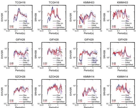
The available strong-motion records at KiK-net sta-tions can be used to evaluate the Earthquake mosta-tions
H/V Spectral Ratio (EHVSR) and Spectral Ratio of Hori-zontal motions between Surface and Bottom of borehole (SRHSB). Therefore, we validate the underground veloc-ity structures identified from SW H/V, if the observed and theoretical EHVSRs and SRHSBs have a good con-sistency. Data analysis about earthquake motions is simi-lar to that of Ducellier et al. (2013). The S-wave parts of strong-motion records for small events (e.g., peak ground acceleration < 100 gal; magnitude < 6; epicenter distance < 200 km) are used to evaluate the power spec-tra in three components, i.e., north–south, east–west,
and up–down. Smoothing with b = 50 by Konno and
Ohmachi (1998) is implemented on the power
spec-tra in three components before finding the square root of power spectral ratios, EHVSR and SRHSB, for each small event. Finally, the observed EHVSRs and SRHSBs are arithmetically averaged over the number of small events. The average EHVSRs and SRHSBs, as well as one standard deviation plus and minus the average one, are shown in Fig. 10. Additional file 2: Tables B1–B6 list the information about small events at six KiK-net stations. Although the number of strong-motion records at a couple of stations is not adequate due to low seismicity, we provide the standard deviations of spectral ratios as rough indicators of variability. The underground velocity structures from surface to bottom of boreholes are used to evaluate the theoretical SRHSBs by the propagation matrix method (Haskell 1960). The underground veloc-ity structures from surface to half-space without cap layer are used to evaluate the theoretical EHVSR which is proportional to the square ratio of transfer functions between S- and P-waves based on diffuse field approxi-mation (Kawase et al. 2011). Smoothing with b = 50 by Konno and Ohmachi (1998) is also implemented on the theoretical SRHSBs and transfer functions.
The effects of attenuation are present in real data, but using damping within the diffuse field approximation is not fully supported by theory. Snieder et al. (2007) showed that the Green’s function can be retrieved from the response to random forcing for a variety of condi-tions, including the extreme case of the diffusion equa-tion. In many practical circumstances, small amounts of damping allow stabilizing results so that the retrieved Green’s functions are consistent with observations (e.g., Lawrence and Prieto 2011). Here we assume the quality
factor for S-wave, Qs = 100, the same as that for FW
H/V. Figure 10 depicts the comparison between observed and theoretical EHVSRs and SRHSBs. The theoretical counterparts were computed for both initial and identi-fied underground velocity structures. The black numeri-cal values in the left bottom of EHVSR and SRHSB panels are the objective functions between observed and theoretical spectral ratios for initial underground veloc-ity structures, and the red ones are the objective func-tion between observed and theoretical spectral ratios for identified underground velocity structures. The smaller objective functions at stations other than GIFH29 and KMMH14 suggest that EHVSRs and SRHSBs for identi-fied underground velocity structures agree better with the observed counterparts. This indicates that the under-ground velocity structures identified from SW H/V are reasonable. The disagreement between observed and the-oretical EHVSRs at GIFH29 and KMMH14, and between observed and theoretical SRHSB at KMMH14 in the short period range, might imply that the assumed damp-ing (Qs = 100) is not appropriate. This issue requires fur-ther scrutiny.
Conclusions
Based on the diffuse field approximation, FW H/V is expressed with the imaginary parts of the Green’s func-tions which incorporate the contribufunc-tions of both body and surface (Rayleigh and Love) waves. SW H/V
is expressed with medium responses of Rayleigh and Love waves according to the Cauchy’s contour integra-tion method. For a given layered medium, the SW H/V
was almost the same as the FW H/V in the short period range. It suggested that the contribution of surface waves trapped in shallow layers was overwhelmingly dominant compared with that of body waves. The largest peak of SW H/V was caused by a local trough of fundamental or higher modes of vertical medium responses of Rayleigh waves. The predominant period of SW H/V is close to but not identical to that of FW H/V unless the imped-ance ratio is large enough. Therefore, the calculation of medium responses of Rayleigh and Love waves gave insight into the contribution of surface waves to full-wave, and the relative contribution between fundamental and higher modes of surface waves.
By adding a cap layer to the bottom of given layered
medium, the SW H/V of cap-layered medium agreed
is about twice as large as the one in the half-space of given layered medium. Because the computation of sur-face waves was significantly fast, SW H/V of cap-layered medium, as a simplified calculation of FW H/V of layered medium without cap layer, was preferable to be applied to identify underground velocity structures.
We applied the SW H/V of cap-layered medium to
identify the underground velocity structures between surface and bottom of boreholes (about several hun-dred meters in depth) at some KiK-net stations where the FW H/Vs did not match with the observed H/Vs. We
employed the identified underground velocity without the cap layer to evaluate the FW H/V. Good consistence between FW H/V with SW H/V of the corresponding cap-layered medium was confirmed. It in turn suggested that SW H/V could be regarded as a simplified calcula-tion of FW H/V to identify underground velocity struc-tures. We further investigated the difference between SW H/V of our approach and DSS-SW H/V proposed on a different premise. Although the amplitude of DSS-SW
H/V was a bit smaller than our SW H/V, the similarity
Finally, we employed the identified underground velocity structures to evaluate earthquake motions of H/V spec-tral ratios based on diffuse field approximation (EHVSR) and spectral ratios of horizontal motions between surface and bottom of boreholes (SRHSB). The good agreement between theoretical and observed EHVSR, and between theoretical and observed SRHSB, indicated that the underground velocity structures identified from SW H/V
of cap-layered medium were well resolved by the new method.
This research implied verifying many details in order not to leave dead ends. The results are quite satisfactory because efficient, faster procedures for modeling and inversion of DFA H/V were developed. Some fundamen-tal issues and significant questions are still open, such as the effect of high damping in soft sediments, the sensitiv-ity to the objective function, and the temporal variance of observations. We need to clarify these issues and open questions before our approach becomes a practical tool for field practitioners. This will require further scrutiny and we are committed in this noble endeavor.
Abbreviations
DFA: diffuse field approximation; H/V: microtremor H/V spectral ratio; FW: full–wave; SW: surface waves; DSS‑SW: surface waves based on distributed surface sources assumption; EHVSR: earthquake motions of H/V spectral ratio; SRHSB: spectral ratio of horizontal motions between surface and bottom of borehole; Tp0: predominant period of fundamental mode; λ0: wavelength
of fundamental mode; Tp0A: “apparent” predominant period of fundamental
mode; λ0A: “apparent” wavelength of fundamental mode; Vs: S‑wave velocity; Vp:
P‑wave velocity.
Authors’ contributions
HW designed this study and drafted the manuscript. KM and HW conducted the microtremor measurement at strong‑motion stations. KI participated in all discussions throughout the study. FS participated in the discussions and interpretation. All authors read and approved the final manuscript.
Author details
1 Earthquake Engineering Group, Geo‑Research Institute, 2‑1‑2, Otemae,
Chuo‑ku, Osaka, Japan. 2 Disaster Prevention Research Center, Aichi Institute
of Technology, Yachigusa 1247, Yakusa‑cho, Toyota, Japan. 3 Instituto de
Ingeniería, Universidad Nacional Autónoma de México, C.U., Coyoacán 04510, CDMX, Mexico.
Additional files
Additional file 1: Table S1. Underground velocity structure model at TCGH16. Table S2. Underground velocity structure model at KMMH03.
Table S3. Underground velocity structure model at GIFH28.
Table S4. Underground velocity structure model at GIFH29.
Table S5. Underground velocity structure model at SZOH26.
Table S6. Underground velocity structure model at KMMH14.
Additional file 2: Table S1. Small events at TCGH16. Table S2. Small events at KMMH03. Table S3. Small events at GIFH28. Table S4. Small events at GIFH29. Table S5. Small events at SZOH26. Table S6. Small events at KMMH14.
Acknowledgements
The authors wholeheartedly thank two anonymous reviewers and the Guest Editor PY Bard, for their detailed review comments and most valuable editing suggestions of the admittedly rough, initial manuscript. Special thanks to the National Research Institute for Earth Science and Disaster Resilience (NIED) for providing PS logging data and strong‑motion records at KiK‑net stations. We thank E. Plata, G. Sánchez, and their team of the Unidad de Servicios de Información (USI) of the Institute of Engineering—UNAM, for locating useful references. This work was supported in part by the Grants‑in‑Aids for Scientific Research (B) (P.I.: Hidenori Kawabe, Grant Number: 16H03144) from the Ministry of Education, Culture, Sports, Science and Technology of Japan, by AXA Research Fund and by DGAPA‑UNAM under Project IN100917. Figures are plotted with Generic Mapping Tools (GMT) (Wessel et al. 2013).
Competing interests
The authors declare that they have no competing interests.
Availability of data and materials
Strong‑motion records at studied KiK‑net stations can be downloaded from the website “http://www.kyoshin.bosai.go.jp/kyoshin/” after a free registration. PS logging data (thickness, P‑wave velocity, S‑wave velocity in each layer) are available from the Web site “http://www.kyoshin.bosai.go.jp/kyoshin/db/ index.html?all”.
Ethics approval and consent to participate Not applicable.
Publisher’s Note
Springer Nature remains neutral with regard to jurisdictional claims in pub‑ lished maps and institutional affiliations.
Received: 21 December 2016 Accepted: 15 November 2017
References
Aki K (1957) Space and time spectra of stationary stochastic waves with spe‑ cial reference to microtremors. Bull Earthq Res Inst 35:415–456 Albarello D, Lunedei E (2013) Combining horizontal ambient vibration compo‑
nents for H/V spectral ratio estimates. Geophys J Int 194:936–951 Arai H, Tokimatsu K (2004) S‑wave velocity profiling by inversion of micro‑
tremor H/V spectrum. Bull Seismol Soc Am 94(1):53–63
Arai H, Tokimatsu K (2005) S‑wave velocity profiling by joint inversion of micro‑ tremor dispersion curve and horizontal‑to‑vertical (H/V) spectrum. Bull Seismol Soc Am 95(5):1766–1778
Baan M (2009) The origin of SH‑wave resonance frequencies in sedimentary layers. Geophys J Int 178:1587–1596
Bonnefoy‑Claudet S, Cornou C, Bard PY, Cotton F, Moczo P, Kristek J, Fäh D (2006a) H/V ratio: a tool for site effects evaluation: results from 1D noise simulations. Geophys J Int 167(2):827–837
Bonnefoy‑Claudet S, Cotton F, Bard PY (2006b) The nature of noise wavefield and its applications for site effects studies: a literature review. Earth Sci Rev 79:205–227
Bonnefoy‑Claudet S, Köhler A, Cornou C, Wathelet M, Bard PY (2008) Effects of Love waves on microtremor H/V ratio. Bull Seismol Soc Am 98(1):288–300 Ducellier A, Kawase H, Matsushima S (2013) Validation of a new velocity
structure inversion method based on horizontal‑to‑vertical (H/V) spectral ratios of earthquake motions in the Tohoku Area, Japan. Bull Seismol Soc Am 103(2A):958–970
Fäh D, Kind F, Giardini D (2001) A theoretical investigation of average H/V ratios. Geophys J Int 145:535–549