Self-Improving Generative Artificial Neural Network
for Pseudo-Rehearsal Incremental Class Learning
Diego Mellado1, , Carolina Saavedra1,2, , Steren Chabert1,2, , Romina Torres3, and Rodrigo Salas1,2,*,
1 Escuela de Ingeniería C. Biomédica. Universidad de Valaraíso. Chile; [email protected],
[email protected], [email protected], [email protected]
2Centro de Investigación y Desarrollo en Ingeniería en Salud, CINGS-UV, Universidad de Valparaíso.
Valparaíso, Chile.
3Engineering Faculty, Universidad Andres Bello, Viña del Mar, Chile; [email protected]
* Corresponding author: [email protected]; Tel.: +56-32-2603658 (R.S.)
Abstract:Deep learning models are part of the family of artificial neural networks and, as such, it suffers of catastrophic interference when they learn sequentially. In addition, most of these models have a rigid architecture which prevents the incremental learning of new classes. To overcome these drawbacks, in this article we propose the Self-Improving Generative Artificial Neural Network (SIGANN), a type of end-to-end Deep Neural Network system which is able to ease the catastrophic forgetting problem when leaning new classes. In this method, we introduce a novelty detection model to automatically detect samples of new classes, moreover an adversarial auto-encoder is used to produce samples of previous classes. This system consists of three main modules: a classifier module implemented using a Deep Convolutional Neural Network, a generator module based on an adversarial autoencoder; and a novelty detection module, implemented using an OpenMax activation function. Using the EMNIST data set, the model was trained incrementally, starting with a small set of classes. The results of the simulation show that SIGANN is able to retain previous knowledge with a gradual forgetfulness for each learning sequence. Moreover, SIGANN can detect new classes that are hidden in the data and, therefore, proceed with incremental class learning.
Keywords:Artificial Neural Networks; Deep Learning; Generative Neural Networks; Incremental Learning; Novelty detection; Catastrophic Interference
1. Introduction
Deep Neural Networks (DNN) are one of the most promising and successful models in recent times due to their performances that have become state of the art in a large number of classification problems that are highly complex. However, there is great concern on the part of the community regarding one of the major limitations of connectionist models, since these models catastrophically forget previously learned patterns when they are learning new data or classes. This limitation prevents these models from being used in real applications that require continuous learning but with a gradual forgetting of past information. The problem of incremental learning has been studied in depth by several authors[1–5], but it is still an open issue.
One of the problems that appear with incremental learning is known asCatastrophic Interference, referring to the inability of an Artificial Neural Network (ANN) to retain previous knowledge while trying to learn a new and unknown task [6]. This problem is known as theStability versus Plasticity Dilemma[7,8] which consists of a concession between the capacity of generalization of the neural network when it self-improve to new samples, and at the same time, trying to preserve its structure in order not to forget previously learned concepts. Some authors have addressed this by using local representations from data[9], while previous works from the authors showed how catastrophic interference might be mitigated by giving flexibility to the artificial neural networks to allow them to
adapt its structure to data, improving their capability to both retain information and reduce catastrophic interference[2,10]. Recentrly, Kemker et al.[11] compare five different mechanisms designed to mitigate catastrophic forgetting in neural networks: regularization, ensembling, rehearsal, dual-memory, and sparse-coding.
Goodfellow et al.[12] have studied the effect of catastrophic interference on deep neural networks, suggesting using the dropout algorithm for balance between learning a new task and remembering a previous task. On the other hand, some recent studies show how generative networks might help on the recognition of unknown classes on multi-class classification tasks [13]. Rebuffi et al. [14] have introduced a new training strategy known as iCaRL to learn classes in an incremental way. The method starts with a training data with a small number of classes presented at the same time, and new classes are added progressively. Y.Li et al.[15] proposed the SupportNet framework that combines DeepLearning with stored samples that contains the essential information of the old data when learning the new information. Z.Li et al.[16] have proposed theLearning without forgetting(LwF) approach where they use data samples coming only of the new prediction tasks without accessing to training data for previously learned tasks. Although the authors do not use data from the previous training sets, the new datasets have some representatives of the previously learned classes, so the approach used by the authors is the rehearsal, that is, they have a small set of samples that they help to retain the concepts of the classes that were previously learned. Recently, Shin et al.[17] proposed the Deep Generative Replay, an architecture consisting of a deep generative model (generator) and a task solving model (solver). The proposed method is able to sequentially train deep neural networks without referring to past data.
On the other hand, there is not much literature on methods that are able to detect the presence of new classes hidden in the data without any supervision [18–20].
In this paper, we propose an end-to-end deep neural network system that acts both as generator and classifier of data to incrementally learn new classes of information present on data by generating samples from previous information, while having the capacity to detect by itself if there is new information present to learn it when needed. This system consists of three major modules: the classifier, the generator, and the novelty detector. The classifier was instantiated with a convolutional neural network that, given an input image, assigns it a label from a set of known categories. The generator module was instantiated with an Adversarial Autoencoder, and its primary task is to generate pseudo-samples to enrich the training set. The classifier was embedded as a detector into the encoder of the latter. Finally, the novelty detector implements an extreme value detector allowing the network to identify whenever if novel information is presented as a new class. At the end, we measure the impact of incremental training with generated data from previously learned information while learning a new task. Further details can be found at D. Mellado’s Thesis [21]
In summary, the main contributions presented in this paper are:
• Designing a neural network model that combines a generative model with a classifier to learn new patterns while reducing the need of storage of training data.
• Introducing a novelty detection model can help to recognize new tasks for incremental learning tasks.
The rest of the paper is organized as follows: we briefly explain in Section2the main methods used to tackle the catastrophic interference problem. In Section3, we explain the architecture of the proposed model, how it works and learns. Then in Section4, we show our results from a series of proposed experiments using a small image dataset to measure its performance when trained incrementally. Finally, we discuss on section5how the model improves on reducing catastrophic interference and we propose future improvements for it on section6.
2. Theoretical Framework
recognize if novel information is present in the data to learn from it. Several training methods have been proposed and used to retain previous knowledge, but some of the most common involve how previous data is presented to the network while training a new task.
2.1. Rehearsal and Pseudorehearsal learning
Rehearsal training in an artificial neural networks involves the collection of data from the previous classes and their incorporation into the model when new data are found and the model needs to be re-trained. One way of doing rehearsal training involves adding a set of the most recently trained examples alongside the new sample, known as Recency Rehearsal[22]. This mechanism allows reinforcing what has the network learned and associated this knowledge with the new data. Another conventional method consists of using a random subset of the previous data alongside the new sample[23]. While this achieves better results than the previous method, there is still some loss of knowledge on most connectionist networks while using these methods. Another point to consider is that these methods require storage of previous training samples. Although it is not an issue on most cases, this becomes a considerable drawback while training vast and increasing databases, as seen in Big Data; where storage of an increasing number of examples can become an is problem. The additional storage may not be biologically plausible because brains are not able to store the exact representation of something that we learn, but rather construct meaning from information, and store it within its neural patterns, while discarding the original information ultimately[24].
Pseudorehearsal, in contrast, does not involve the use of previously trained items and instead, using randomly generated elements that act in a similar form to the original training data[23]. These random elements usually are inputted into the previously trained network to get their outputs and added to the new item to train the network for the new set. This method allows the training of new data by approximating the previous information whenever is needed[25] One caveat of this problem was presented by Ans et al.[26], where they demonstrated that using only random samples can cause problems while generalizing on increasing data due to their noisy origin, effectively destroying what the previous knowledge was on the model. So, a secondary network in parallel is needed to create pseudo-samples for the primary network to learn from representations.
This method, compared to rehearsal learning, is more biologically plausible due to not requiring to store all previous data directly, and using stochastic processes to generate them, giving the idea of “evoking” the concept of what the neural network have already learned. This evoking allows it to approximate old information, by sampling the behavior of how the neural network should behave on these inputs, allowing the consolidation of information while learning a new task[25]
Previous research by the authors[27] showed that pseudorehearsal has slightly lower performance when training with pseudo-samples in comparison to a rehearsal approach. However, on both methods, the classifier has a peak accuracy of almost 90%, when using as few as 10% from a total of 512 generated samples per trained class, showing that this method can be useful for incremental training of deep neural networks without having to store or generate a significant amount of data. Atkinson et al.[28] expanded on this idea by using a Generative Adversarial Network to generate data to train a model incrementally, whereas Besedin et al.[29] expanded this model and analyzed the impact of regeneration of images while training incrementally.
Further details about the main challenges on the incremental learning and catastrophic forgetting are given in Parisi et al.[30].
2.2. Variational Autoencoders for Image Generation
P(X) =
Z
P(X|z;θ)P(z)dz (1)
WhereP(X|z)is a set of functions, parameterized byθ, or the parameters we want to optimize. This allow to sample fromP(z)with a high probability to obtain a value fromX[32].
This latent vector acts as a prior that enables the decoder to map information onto a representation, using the maximum likelihood to the image. Both encoder and decoder network uses a similar structure to recreate an output with similar features from the initial input, as an autoencoder structure.
To optimize these networks, the Kullback-Leibler distance between latent vectorzand a defined random distribution is minimized (Equation2).
KL[Q(z)||P(z|X)] =Ez∼Q[logQ(z)−logP(z|X)] (2) whereP(z|X)∼ Z(µ,σ+e),µandσare obtained as output from the encoder,eis stochastic noise, andQ(z)is usually similar to a Gaussian distributionN(0,I), beingIan identity matrix. Moreover, the difference between the input and its reconstruction (usually the Mean Squared Error or the binary cross-entropy between input and output) is reduced, allowing to decode spatial information from a reduced, stochastic source and with similar characteristics to a real input[32].
These types of networks are widely used for generating small images by encoding image features and enabling to generate new images with small variations on these features[33,34]. Newer variations, try to improve encoding by making them indistinguishable from real information. Neural Network models such as[35,36] use a discriminator network, similar to Generative Adversarial Network models, to create generated samples that are similar to real examples. Adversarial models allow this by competition between the generator and a discriminator network that identifies if the input is generated or belongs to a real set, balancing each other[37].
2.3. Novelty recognition
Novel pattern recognition is the field that studies how an algorithm or system can recognize if a pattern is unknown to it, compared to a set of previously learned patterns[38]. Some of these techniques are commonly used for outlier detection, due to how these events deviate from what the system usually outputs from an input. The detection can be probabilistic, distance-based, reconstruction-based, from domain or by measuring information content, among others[39].
Novelty recognition has been recently used on Deep Neural Network (DNN) models to improve detection of new information available on inference. Richter et al.[40] for example, developed an auto-encoder model for novelty recognition for a reinforcement learning problem. This algorithm can identify if the environment is similar to the training environment, improving navigation on an autonomous system when trying to identify its navigation confidence.
Novelty detection can be used as a tool for recognition of an object from a universe of different unknown objects, considering the category unknown as a possibility, known as Open-set Recognition. Bendale et al.[41] created a DNN for open-set recognition by measuring the activation distance of the output layer from a classifier compared to the maximum response of a specific class and using Extreme-Value Theory to model the probability of rejection of the input from a perceived class.
Extreme Value Theory involves the study of extrema, or maximum or minimum values, in probabilistic distributions; commonly used for rejection of outliers. A general representation of the cumulative distribution function of an extreme value distribution is in Equation3.
P[X≤x] =
1+ξ
x−µ
σ 1
ξ
(3)
where 1+ξ x−µ
σ
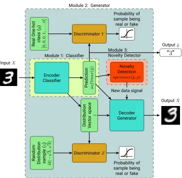
Module 2: Generator
Module 1: Classifier Module 3:Novelty Detector
InputX Encoder Classifier Pr ediction sof tmax (ˆ y ) Distribution Vect or
space ˆz Decoder
Generator
OutputXˆ
“
3
”
Outputyˆ
Novelty Detection
openmax(ˆy, ρ)
Real One-hot class ( y ) 0, 0 , 0 , 1 ,. .. , 0
Random Distribution sample
( z ) U ( − √ 3 , √ 3) DiscriminatorY DiscriminatorZ Probability of sample being real or fake
Probability of sample being real or fake New data signal
Figure 1.SIGANN model, using a Semi-supervised Adversarial Autoencoder structure
ξ→ −∞or∞, becomes a Gumbel-type distribution [42]. As activation parameters in a neural network are bounded, their distribution reduces to a Weibull distribution[43]. The probability of rejection of an outlier is given by the output of this distribution, in relation to how data is distributed within it.
Novelty detection algorithms have also been used with Adversarial Autoencoders (AAE) for measurement of the likelihood of images belonging to the training set, allowing for better sample generation[19].
3. Proposal
Our proposed neural network system, “Self-Improving Generative Artificial Neural Network” (SIGANN)1, consists of 3 major sub-structures: A classifier, a generator and a novelty detector working in conjunction, to learn and identify unknown data from a starting subset of a dataset, and training it to learn new classes. For both the classifier and generator, we implemented a semi-supervised AAE model, based on the structure presented on[35] for semi-supervised training, and added the novelty detector.
To incrementally train SIGANN, we train the classifier and generator at the same time, as a standard AAE model; and fit the mean activations for each initial class on our novelty detector by inferring on the training set at the end of the training process. On inference, the novelty detector checks if new information belongs to a new class using the novelty detector. If so, it temporarily
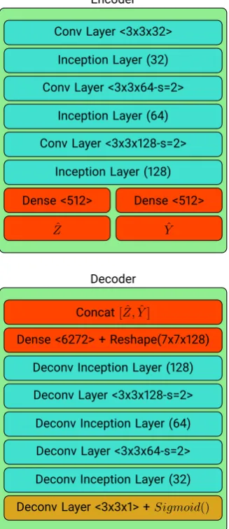
Encoder
Conv Layer <3x3x32> Inception Layer (32) Conv Layer <3x3x64-s=2>
Inception Layer (64) Conv Layer <3x3x128-s=2>
Inception Layer (128)
Dense <512> Dense <512>
ˆ
Z Yˆ
Decoder
Concat[ ˆZ,Yˆ]
Dense <6272> + Reshape(7x7x128) Deconv Inception Layer (128) Deconv Layer <3x3x128-s=2> Deconv Inception Layer (64) Deconv Layer <3x3x64-s=2> Deconv Inception Layer (32) Deconv Layer <3x3x1> +Sigmoid()
Algorithm 1SIGANN Model training
Require: Set of initial dataXtrainand output classesytrain∈ {1, . . . ,C}
1: Uniform Distribution GeneratorZ=U(−√3,√3)of sample lengthn
2: Train Adversarial Autoencoder: ˆX, ˆz, ˆy= AAE(Xtrain,ytrain,Z)
3: forc=1,. . . ,Cdo
4: Get Mean Activation of trained samplesµc=mean(yˆ∈c)
5: Compute distance of each output of classc:dc=|ycˆ −µc|
6: Fitdcto Weibull distributionWcand get parametersρc= (κc,λc)
7: whileReceiving new dataXnewdo
8: Evaluate samples of dataXnewon inference: ˆy= AAEenc(Xnew)
9: Revise OpenMax activation of data:y?=OpenMax(yˆ,ρ,e=0.95)
10: ify?=C+1then
11: Store inputX?and outputy?
12: Generate samplesXgenfrom classesygen∈ {1, . . . ,C}
13: Evaluate generated samples: ˆygen=AAEenc(Xgen)
14: ifygenˆ =ygenandP(ygenˆ =c|X)>0.9then
15: StoreXgen,ygen
16: else
17: DiscardXgen,ygenand Re-generate 18: Update Number of classes:C=C+1
19: Re-train Adversarial Autoencoder with new and generated data: ˆX, ˆz, ˆy = AAE(Xgen+
X?,ygen+y?,Z)
20: Fit new class and samples to Weibull distribution
21:
stores the sample for future training, as the generator starts sampling a set of previous knowledge representations for the next training step. This set is used in conjunction with all detected new samples, and the categorical output layer from the classifier is expanded to add the new class. Finally, the network is trained for a defined number of epochs, learning new information without loss of previous knowledge.
The complete operation of our method is presented on Algorithm1and the structure of the Semi-supervised AAE model used in conjunction with the novelty detector is shown on Figure1. In the following subsections we explain each module.
3.1. Module 1: Classifier
The classifier module consists of an encoder unit which is shared with the generator module, and the SoftMax function that output the predicted class of imageX. This module also outputs the encoded style information for the generator module.
3.2. Module 2: Generator
The generator module is based on an Adversarial Autoencoder, whose units are the encoder structure from the classifier, the decoder, and the distribution and categorical discriminators. These structures allow SIGANN to learn spatial information and generate real-looking samples for usage on future training operations.
Both ˆzand ˆyoutputted from the encoder structure from input imageX, are concatenated and used as an input for the decoder structure, which mirrors the encoding network structure using deconvolution filters, outputting a decoded image ˜X. The generator can encode information from random noise to generate almost real samples by training two discriminator networksZandY(as shown on Figure1) which try to differentiate between the true categorical and random uniform priors and the generated inputs from the encoder [35]. These discriminators are built using two sets of 2-layer perceptron networks with a binary output, to identify if the distribution sampleZand categorical sampleycomes from real or generated samples. The Generator ultimately tries to fool the discriminators, by creating encoding vectors with a similar distribution to the distribution sampleZ and categorical outputy, to decode them into a real image, similar to the original.
The complete loss functionLused for the training is obtained as the aggregation of the following loss functions: 1) the reconstruction lossLrec, obtained from the binary cross-entropy between the original imageXand the generated image ˆX; 2) the discriminative lossesLdisfrom both the encoding vector ˆzand the class ˆydiscriminators; 3) the generative lossLgenfrom the generator when fooling the discriminators; and 4) the classification lossLclsfrom the classifier.
3.3. Module 3: Novelty Detector
The novelty detector consists of the joint action from the Meta-recognition and OpenMax algorithms. After training the AAE for a defined number of classes, we evaluate data to classify it. Generally, if a sample is from a new, unknown class, the classifier should not be able to identify it as such. So, we replace on the inference stage the activation function of the classifier with an OpenMax function [41] to do novelty detection. This activation function was initially designed as a replacement for SoftMax activation on open-set recognition networks.
By using theMeta-Recognitionalgorithm presented by [43] as a basis, this function fits data into a Weibull distribution to obtain the probability of each sample of being on a high or low tail of the set, selecting theηvalues from the tail of the distribution. This fitting is done using the Euclidean distance between each training sample’s output activation logit, or the output from the last layer of a classifier before applying SoftMax activation function; and the mean activation of all samples from classc, obtaining the scale and shape parameters of the Weibull distribution for classc. By definingρc as these parameters, we use the Weibull CDF on the Euclidean distance between the mean activation logits of classµcfrom the training set and the logits obtained on inference. We obtain this value for the topαclasses, obtaining weightsω(x)for each class of the logit output. The sum difference between the original and corrected logits gives us the “unknown logit” which is then evaluated using the SoftMax equation (Equation4).
P(z)j = ezj
∑K k=1ezk
j=1, . . . ,K (4)
Algorithm 2Meta-Recognition Algorithm
Require: Logits from the final layer from each classvc(x) = v1(x). . .vN(x)from training phase; Number of extreme values to fitη
1: forc=1 . . .Ndo
2: Compute Mean Activation :µc=mean(vc)
3: Fit to Weibull :ρc= (κc,λc) =FitHigh(kvc−µck,η)
4: returnµcandρcfor each class
Algorithm 3OpenMax Algorithm
Require: Logits from the final layer from each classvc(x) =v1(x). . .vC(x)from evaluation;αnumber of top classes to revise.
1: Execute Algorithm2of the Meta-Recognition to obtain the Meanµc and Weibull parameters
ρc= (κc,λc)for each classc
2: fori=1, . . . ,αdo
3: s(i) =argsort(vc(x))
4: ωs(i)(x) =1−α−αie−
k
vi(x)−µs(i)k
λs(i)
κs(i)
5: Revise activations: ˆv(x) =v(x)◦ω(x)
6: Define ˆvnew(x) =∑i(vi(x)−vˆi(x))
7: Pˆ(y=j|x) = evcˆ(x)
∑N
c=0evcˆ(x)
8: Lety?=argmaxiP(y=i|x)
9: returnNew class ify?=C+1 orP(y=y?|x)<e
network on new data. The Meta-Recognition and OpenMax algorithms are presented on Algorithm2 and on Algorithm3respectively.
With all unknown information identified, we then use the generator to create a balanced set of generated samples from the previously learned classes, adding them to the new training set, and start training with the new data. This allows our model to “finetune” their weights for the old data and accommodate for new features that might help activate the corresponding output for the new class.
4. Experiments
To assess SIGANN’s learning capabilities, three experiments were proposed. First, we measure the rate at which the method forgets previously learned classes. Second, we study the ability of the method to detect new unknown classes. And third, we study how long the method could last without forgetting catastrophically the former classes under a continual learning setting.
We used as a benchmark for our experiments the EMNIST dataset2[44], an extension of the original MNIST dataset for handwritten digits, with the inclusion of handwritten characters and numbers from the NIST Special Database 19. The EMNIST Balanced subset, is comprised of 131600 character images, with 47 different classes from 0-9, A-Z and a set of lowercase a-z characters different from their uppercase counterparts. For the initial training task, we trained the model using the number classes and incrementally adding each letter in alphabetical order at each training stage.
For all experiments, our network was trained for 25 epochs for each training step, using Adam Optimizer, with an initial learning rate of 0.001 and β value of 0.9. The dataset was augmented
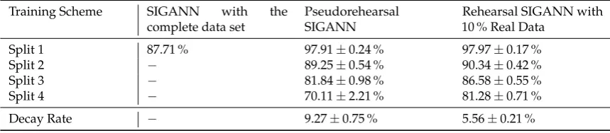
Table 1.Accuracy evaluated in the test sets using EMNIST partition in four splits Training Scheme SIGANN with the
complete data set
Pseudorehearsal SIGANN
Rehearsal SIGANN with 10 % Real Data
Split 1 87.71 % 97.91±0.24 % 97.97±0.17 %
Split 2 − 89.25±0.54 % 90.34±0.42 %
Split 3 − 81.84±0.98 % 86.58±0.55 %
Split 4 − 70.11±2.21 % 81.28±0.71 %
Decay Rate − 9.27±0.75 % 5.56±0.21 %
while training with random padding and contrast of each image. For all the experiments, we have separated the dataset, for each stage, in training and test sets and we report the average and standard deviation performance of 15 runs in the test set. Our setup was an HP Proliant Workstation with Intel Xeon ES-2620 CPU with 16GB of RAM and an NVIDIA GeForce GTX960 GPU; and implemented on TensorFlow 1.8 using Python 3.6.
4.1. Experiment 1: Does the method gradually forgets?
As a first experiment, our model was trained to learn iteratively on splits of these datasets, in order to study if our network can retain previous information while learning new data and how much information is lost while learning a new task using only what the model remembers of the previous task. The dataset was split into four parts with an even number of classes each. The network was trained using an initial set. After training each set, we evaluated its classification accuracy and generated a set of images from each learned class, in order to append it to the new learning task. The generated images were selected for training if the predicted class from the classifier matched the input class from the generator. On the following steps, we retrained the model with the next batch of new classes, plus a defined number of generated data around 75% of the amount of the original training samples for each class from the previous set. We decided to set this value due to an unbalancing issue with the previously learned classes while training the new set.
As a base metric, the obtained accuracy for our classifier while evaluating the complete dataset was 87.71% on EMNIST; this result is similar to state of the art on this particular subset. While training the generated set, the accuracy of each training iteration lowered in a constant decay per training step of around 9.27±0.75%. When trained to add a small subset of the original data to the generated samples, the decay rate on each training step is lowered to almost half, as shown in Table1. This decay can be explained as a gradual interference effect of how information is learned within the model and related to how plastic is our proposed model while learning new features of the newer classes. As a comparison, we trained the same model with generated samples and an additional 10% of randomly sampled original training data, to test performance in semi-rehearsal training.
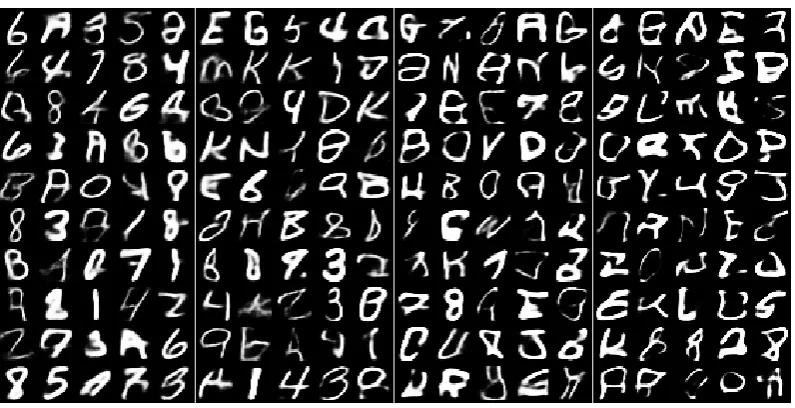
This gradual loss of information can be seen in the generated samples from the model in figure3. On each training split, the recently learned task starts with a better definition of its shape style due to how it is encoded on the distribution vector. On following splits, its shape starts to lose form due to the increase a number of classes information within the encoding space.
4.2. Experiment 2: is the method able to detect new unknown classes?
Figure 3.Generated Samples on each training cycle (5 columns per training cycle)
Our novelty detector, when trained with only numbers, detects up to 55 % of the unknown data on classes with higher distance to what is already known. The accuracy while classifying without novelty detection is around 61 %, consistent with the number of test data from the original set since almost all failures come from the unknown class. Using OpenMax, accuracy raises from 60.08±4.04 % at its lowest detecting the letter Z, and up to 80.035±4.480 % detecting the letter C. On average, the mean accuracy using OpenMax is 71.64±5.75 %. The detector on average can identify around 37.065±15.770 % of the total samples of new data presented on inference, using a rejection threshold ofe=0.95. Although in some cases the novelty detector has a relatively low accuracy in the detection of new classes, it is required only a small number of samples to be recognized as novel to begin the process of increasing the model to learn this new class.
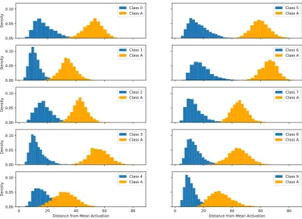
By measuring the Euclidean distance between each activation logit from a new class and the mean activation from each training class, we can infer how similarity can impact on the misclassification of a sample. On Figure4, we compare the distances between character uppercase A and each number character from the dataset. This character gets typically misclassified with the number 4, and its distance distribution intersects with a large part of the activation distances from the training set. Still, a large chunk of the set is further than the maximum tail of class 4, and thus, those examples have a higher probability to be rejected and reclassified as a new class.
On Table2, we show the mean percentage of the total number of samples from each character detected by the novelty detector. The character uppercase O is the most complex to accurately identify as a new class, due to it’s similarity to the number 0, this trend is noticeable with other similar number shaped characters, such as I, H, S, and Z, being similar to the numbers, 1, 8, 5 and 2 respectively.
While this detection can be improved using lower thresholds, the detector starts to misclassify previous classes more. Thisevalue achieves a balance between good novelty detections and accuracy on previous information. This shows that whenever we are using the OpenMax algorithm as a novelty detector, then we can safely detect new data if it is different enough to the learned set.
4.3. Experiment 3: How long the method could last?
0.00 0.05 0.10
De
nsi
ty Class 0Class A Class 5Class A
0.00 0.05 0.10
De
nsi
ty
Class 1
Class A Class 6Class A
0.00 0.05 0.10
De
nsi
ty Class 2Class A Class 7Class A
0.00 0.05 0.10
De
nsi
ty Class 3Class A Class 8Class A
0 20 40 60 80 Distance from Mean Activation
0.00 0.05 0.10
De
nsi
ty
Class 4 Class A
0 20 40 60 80 Distance from Mean Activation
Class 9 Class A
Figure 4.Histogram of activation distances between each training class and the new character class A
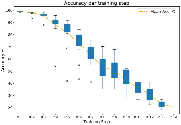
When combining both our network and novelty detector, we start to see a slow decline in accuracy on each evaluation step, mostly due to an increase in noise on the network’s generated samples from earlier tasks, this is an effect of using generated samples of already generated data. Figure5shows that for at least three training iterations, our model can adequately retain previous information while learning a new task, without any effects caused by generator noise. Afterwards, the network starts its gradual loss of information, and lowering its accuracy with a rate of 7 % per training step.
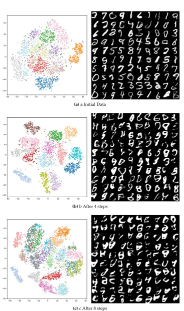
This information loss can be explained by how information is encoded on a limited space, defined on ˆz, as shown in Figure6.
When trained on the initial classes (Figure6a), each character clusters within the distribution space, allowing to generate different characters as the encoding vector ˆzis defined within it. As the number of new classes increases, information regarding shape, style, and class is clustered within a reduced space, thus reducing the variability of the generated samples on decoding. This effect is shown in Figure6band6c, where boundaries between clusters are muddled, and thus reducing differences between outputs from different classes. In addition to this, as previous information is continuously retrained without the original content, this reduction in variability create less-defined outputs, impacting on how the network can retain long-term information on about old data.
5. Discussion
Table 2.Percentage of new class identification for each non-number character images on EMNIST after training with number images
char % char %
A 49.91±7.66 % T 32.82±9.12 % B 28.76±8.88 % U 44.44±13.44 % C 61.49±10.40 % V 41.43±11.63 % D 45.71±27.46 % W 47.37±8.36 % E 45.42±8.17 % X 47.07±11.92 % F 60.38±7.66 % Y 19.45±5.03 % G 38.38±7.44 % Z 8.27±3.54 % H 14.92±7.78 % a 46.16±9.43 % I 14.11±11.89 % b 19.83±7.69 % J 40.46±6.87 % d 51.22±8.56 % K 45.56±7.56 % e 57.91±6.29 % L 11.38±6.33 % f 60.82±8.16 % M 60.21±8.85 % g 25.36±4.39 % N 42.64±8.00 % h 43.84±8.01 % O 35.84±37.46 % n 54.74±9.65 % P 42.73±7.54 % q 22.27±4.51 % Q 48.37±8.46 % r 55.91±10.83 % R 36.09±6.66 % t 29.99±8.64 % S 15.38±8.06 %
adjusting by the rejection probability using a Weibull distribution, we can effectively select examples from new information.
Despite being able to learn and retain information for a limited number of training iterations without significant loss, when trained continuously using only a small number of generated samples, an effect of gradual forgetting is present. The decay rate presented while training with this effect is significantly lower than expected, considering the risk of catastrophic interference caused from using no original training samples from previous training iterations, and could be mitigated using a higher number of data or improving the novelty detector. This process can be compared on how memory is impacted when learning, as previous knowledge is harder to recall after learning new, more recent information, due to interference while encoding both what is previously known and the new stimulus. With fewer samples to re-order information alongside what is known, the model shows a similar effect to when there is less time to reorganize information on the brain between learning epochs [45].
The difference between Rebuffi et al. [14] and Li’s et al. [16] works with respect to our proposal relies upon that our method does not consider a memory module and it has the ability to detect whenever a new class appears in the data set. It is important to note that our SIGANN proposal forgets at a higher rate than iCaRL due mainly to the pseudorehearsal approach of our method where the SIGANN model does not use any sample of the classes that were previously learned. However when we use 10% of new samples of the class we are able to have comparable results (Rehearsal approach). Thus, our approach could be a step towards achieving a self-training neural network, able to do life-long learning of newer information as it arises.
6. Conclusion
In this work, we proposed a neural network system which combined the capabilities of Adversarial Autoencoders to generate and classify information, and a novelty detection algorithm for identification of unknown data; to incrementally learn new information in an unsupervised way and reducing the need of storage of previously-learned data.
It 1 It 2 It 3 It 4 It 5 It 6 It 7 It 8 It 9 It 10 It 11 It 12 It 13 It 14
Training Step
20 30 40 50 60 70 80 90 100
A
cc
ur
ac
y
%
Accuracy per training step
Mean Acc. %
Figure 5.Accuracy of incremental training on each training step with random character images.
learning of streaming data in a semi-supervised way, allowing training of new information without having to store information and when needed.
In future works, we expect to extend our model to more complex image classification datasets such as CIFAR and ImageNet. On the other hand, future work will improve the long-term retention of prior information to reduce the effects of gradual forgetfulness of information loss when learning new classes; as this is one of the most significant challenges for achieving life-long learning on an increasing number of data classes. Also, giving the system a long-term memory module might improve on how sample variance is stored within the distributional space. Achieving this, might improve in stability and allow to generate better samples to improve itself continually.
Author Contributions:conceptualization, D. Mellado, R. Salas and C. Saavedra; methodology, D. Mellado, R. Salas, C. Saavedra, S. Chabert and R. Torres; software, D. Mellado, R. Salas and R. Torres; validation, D. Mellado, R. Salas, C. Saavedra, R. Torres and S. Chabert; writing–original draft preparation, D. Mellado; writing–review and editing, R. Salas, C. Saavedra, R. Torres, S. Chabert; supervision, R. Salas.
Funding:The authors acknowledge the support of CONICYT + PAI/CONCURSO NACIONAL INSERCIÓN EN LA ACADEMIA, CONVOCATORIA 2014 + Folio (79140057), FONDEF ID16I10322 and REDI170367 from CONICYT. The work of S. Chabert was funded by CONICYT - PIA - Anillo ACT1416.
Conflicts of Interest:The authors declare no conflict of interest
References
1. Polikar, R.; Upda, L.; Upda, S.S.; Honavar, V. Learn++: An incremental learning algorithm for supervised neural networks. IEEE transactions on systems, man, and cybernetics, part C (applications and reviews)2001,
31, 497–508.
2. Salas, R.; Moreno, S.; Allende, H.; Moraga, C. A robust and flexible model of hierarchical self-organizing maps for non-stationary environments.Neurocomputing2007,70, 2744–2757.
3. Santoro, A.; Bartunov, S.; Botvinick, M.; Wierstra, D.; Lillicrap, T. Meta-learning with memory-augmented neural networks. International conference on machine learning, 2016, pp. 1842–1850.
4. Thrun, S. Is learning the n-th thing any easier than learning the first? Advances in neural information processing systems, 1996, pp. 640–646.
−80 −60 −40 −20 0 20 40 60 80 −60
−40 −20 0 20 40 60
(a)a Initial Data
−80 −60 −40 −20 0 20 40 60
−80 −60 −40 −20 0 20 40 60
(b)b After 4 steps
−80 −60 −40 −20 0 20 40 60 80
−80 −60 −40 −20 0 20 40 60
(c)c After 8 steps
6. McCloskey, M.; Cohen, N.J. Catastrophic Interference in Connectionist Networks: The Sequential Learning Problem. InPsychology of Learning and Motivation; Bower, G.H., Ed.; Academic Press, 1989; Vol. 24, pp. 109–165.
7. Grossberg, S.Studies of Mind and Brain: Neural Principles of Learning, Perception, Development, Cognition, and Motor Control; Reidel Press., 1982.
8. Mermillod, M.; Bugaiska, A.; Bonin, P. The stability-plasticity dilemma: investigating the continuum from catastrophic forgetting to age-limited learning effects. Frontiers in Psychology 2013, 4. doi:10.3389/fpsyg.2013.00504.
9. French, R.M. Semi-distributed Representations and Catastrophic Forgetting in Connectionist Networks.
Connection Science1992,4, 365–377. doi:10.1080/09540099208946624.
10. Salas, R.; Saavedra, C.; Allende, H.; Moraga, C. Machine fusion to enhance the topology preservation of vector quantization artificial neural networks. Pattern Recognition Letters 2011, 32, 962 – 972. doi:https://doi.org/10.1016/j.patrec.2011.01.020.
11. Kemker, R.; McClure, M.; Abitino, A.; Hayes, T.L.; Kanan, C. Measuring catastrophic forgetting in neural networks. Thirty-second AAAI conference on artificial intelligence, 2018.
12. Goodfellow, I.J.; Mirza, M.; Xiao, D.; Courville, A.; Bengio, Y. An Empirical Investigation of Catastrophic Forgetting in Gradient-Based Neural Networks. arXiv:1312.6211 [cs, stat]2013. arXiv: 1312.6211.
13. Ge, Z.; Demyanov, S.; Chen, Z.; Garnavi, R. Generative OpenMax for Multi-Class Open Set Classification.
arXiv:1707.07418 [cs]2017. arXiv: 1707.07418.
14. Rebuffi, S.A.; Kolesnikov, A.; Lampert, C.H. iCaRL: Incremental Classifier and Representation Learning.
2017 IEEE Conference on Computer Vision and Pattern Recognition (CVPR)2017, pp. 5533–5542.
15. Li, Y.; Li, Z.; Ding, L.; Yang, P.; Hu, Y.; Chen, W.; Gao, X. Supportnet: solving catastrophic forgetting in class incremental learning with support data. arXiv preprint arXiv:1806.029422018.
16. Li, Z.; Hoiem, D. Learning without Forgetting.IEEE Transactions on Pattern Analysis and Machine Intelligence 2018,40, 2935–2947.
17. Shin, H.; Lee, J.K.; Kim, J.; Kim, J. Continual learning with deep generative replay. Advances in Neural Information Processing Systems, 2017, pp. 2990–2999.
18. Cherti, M.; Kegl, B.; Kazakci, A. Out-of-Class Novelty Generation : An Experimental Foundation. 2017 IEEE 29th International Conference on Tools with Artificial Intelligence (ICTAI), 2018, pp. 1312–1319. 19. Leveau, V.; Joly, A. Adversarial autoencoders for novelty detection. PhD thesis, Inria-Sophia Antipolis,
2017.
20. Skvára, V.; Pevný, T.; Smídl, V. Are generative deep models for novelty detection truly better? Proceedings of the ACM SIGKDD Workshop on Outlier Detection De-constructed (KDD-ODD 2018), 2018.
21. Mellado, D. A Biological Inspired Artificial Neural Network Model for Incremental Learning with Novelty Detection. Master’s thesis, Biomedical Engineering, Universidad de Valparaiso, Chile, 2018.
22. Ratcliff, R. Connectionist models of recognition memory: Constraints imposed by learning and forgetting functions. Psychological review1990,97, 285–308.
23. Robins, A. Catastrophic forgetting, rehearsal and pseudorehearsal. Connection Science1995,7, 123–146. 24. Freeman, W.J. How and Why Brains Create Meaning From Sensory Information. International
Journal of Bifurcation and Chaos 2004, 14, 515–530, [https://doi.org/10.1142/S0218127404009405]. doi:10.1142/S0218127404009405.
25. Robins, A.; McCallum, S. The consolidation of learning during sleep: comparing the pseudorehearsal and unlearning accounts. Neural Networks1999,12, 1191–1206.
26. Ans, B.; Rousset, S. Avoiding catastrophic forgetting by coupling two reverberating neural networks. Comptes Rendus de l’Académie des Sciences - Series III - Sciences de la Vie1997,320, 989–997. doi:10.1016/S0764-4469(97)82472-9.
27. Mellado, D.; Saavedra, C.; Chabert, S.; Salas, R., Pseudorehearsal Approach for Incremental Learning of Deep Convolutional Neural Networks. InComputational Neuroscience: First Latin American Workshop, LAWCN 2017, Porto Alegre, Brazil, November 22–24, 2017, Proceedings; Springer International Publishing: Cham, 2017; pp. 118–126. doi:10.1007/978-3-319-71011-2_10.
29. Besedin, A.; Blanchart, P.; Crucianu, M.; Ferecatu, M. Evolutive deep models for online learning on data streams with no storage. Proceedings of the Workshop on IoT Large Scale Learning from Data Streams co-located with the 2017 European Conference on Machine Learning and Principles and Practice of Knowledge Discovery in Databases (ECML-PKDD 2017), 2017, p. 12.
30. Parisi, G.I.; Kemker, R.; Part, J.L.; Kanan, C.; Wermter, S. Continual lifelong learning with neural networks: A review.Neural Networks2019.
31. Kingma, D.P.; Welling, M. Auto-encoding variational bayes. arXiv preprint arXiv:1312.61142013. 32. Doersch, C. Tutorial on variational autoencoders. arXiv preprint arXiv:1606.059082016.
33. Gregor, K.; Danihelka, I.; Graves, A.; Rezende, D.J.; Wierstra, D. DRAW: A Recurrent Neural Network For Image Generation. arXiv:1502.04623 [cs]2015.
34. Kulkarni, T.D.; Whitney, W.F.; Kohli, P.; Tenenbaum, J. Deep convolutional inverse graphics network. Advances in Neural Information Processing Systems, 2015, pp. 2539–2547.
35. Makhzani, A.; Shlens, J.; Jaitly, N.; Goodfellow, I.; Frey, B. Adversarial Autoencoders. arXiv:1511.05644 [cs] 2015. arXiv: 1511.05644.
36. Creswell, A.; Bharath, A.A.; Sengupta, B. Conditional Autoencoders with Adversarial Information Factorization. arXiv preprint arXiv:1711.051752017.
37. Goodfellow, I.; Pouget-Abadie, J.; Mirza, M.; Xu, B.; Warde-Farley, D.; Ozair, S.; Courville, A.; Bengio, Y. Generative adversarial nets. Advances in neural information processing systems, 2014, pp. 2672–2680. 38. Markou, M.; Singh, S. Novelty detection: a review—part 1: statistical approaches. Signal processing2003,
83, 2481–2497.
39. Pimentel, M.A.; Clifton, D.A.; Clifton, L.; Tarassenko, L. A review of novelty detection. Signal Processing 2014,99, 215–249.
40. Richter, C.; Roy, N. Safe visual navigation via deep learning and novelty detection. Proc. of the Robotics: Science and Systems Conference, 2017.
41. Bendale, A.; Boult, T.E. Towards open set deep networks. Proceedings of the IEEE Conference on Computer Vision and Pattern Recognition, 2016, pp. 1563–1572.
42. Kotz, S.; Nadarajah, S.Extreme Value Distributions: Theory and Applications; Imperial College Press, 2000. 43. Scheirer, W.J.; Rocha, A.; Michaels, R.; Boult, T.E. Meta-Recognition: The Theory and Practice of Recognition
Score Analysis. IEEE Transactions on Pattern Analysis and Machine Intelligence (PAMI)2011,33, 1689–1695. 44. Cohen, G.; Afshar, S.; Tapson, J.; van Schaik, A. EMNIST: an extension of MNIST to handwritten letters.
arXiv:1702.05373 [cs]2017. arXiv: 1702.05373.