R E S E A R C H
Open Access
Training sequence design for MIMO channels:
an application-oriented approach
Dimitrios Katselis
1*, Cristian R Rojas
1, Mats Bengtsson
1, Emil Björnson
1, Xavier Bombois
2,
Nafiseh Shariati
1, Magnus Jansson
1and Håkan Hjalmarsson
1Abstract
In this paper, the problem of training optimization for estimating a multiple-input multiple-output (MIMO) flat fading channel in the presence of spatially and temporally correlated Gaussian noise is studied in an application-oriented setup. So far, the problem of MIMO channel estimation has mostly been treated within the context of minimizing the mean square error (MSE) of the channel estimate subject to various constraints, such as an upper bound on the available training energy. We introduce a more general framework for the task of training sequence design in MIMO systems, which can treat not only the minimization of channel estimator’s MSE but also the optimization of a final performance metric of interest related to the use of the channel estimate in the communication system. First, we show that the proposed framework can be used to minimize the training energy budget subject to a quality
constraint on the MSE of the channel estimator. A deterministic version of the ‘dual’ problem is also provided. We then focus on four specific applications, where the training sequence can be optimized with respect to the classical channel estimation MSE, a weighted channel estimation MSE and the MSE of the equalization error due to the use of an equalizer at the receiver or an appropriate linear precoder at the transmitter. In this way, the intended use of the channel estimate is explicitly accounted for. The superiority of the proposed designs over existing methods is demonstrated via numerical simulations.
1 Introduction
An important factor in the performance of multiple antenna systems is the accuracy of the channel state infor-mation (CSI) [1]. CSI is primarily used at the receiver side for purposes of coherent or semicoherent detection, but it can be also used at the transmitter side, e.g., for precoding and adaptive modulation. Since in communi-cation systems the maximization of spectral efficiency is an objective of interest, the training duration and energy should be minimized. Most current systems use train-ing signals that are white, both spatially and temporally, which is known to be a good choice according to several criteria [2,3]. However, in case that some prior knowl-edge on the channel or noise statistics is available, it is possible to tailor the training signal and to obtain a signif-icantly improved performance. Especially, several authors have studied scenarios where long-term CSI in the form
*Correspondence: [email protected]
1ACCESS Linnaeus Center, School of Electrical Engineering, KTH Royal Institute of Technology, Stockholm SE-100 44, Sweden
Full list of author information is available at the end of the article
of a covariance matrix over the short-term fading is avail-able. So far, most proposed algorithms have been designed to minimize the squared error of the channel estimate, e.g., [4-9]. Alternative design criteria are used in [5] and [10], where the channel entropy is minimized given the received training signal. In [11], the resulting capacity in the case of a single-input single-output (SISO) channel is considered, while [12] focuses on the pairwise error probability.
Herein, a generic context is described, drawing from similar techniques that have been recently proposed for training signal design in system identification [13-15]. This context aims at providing a unified theoretical frame-work that can be used to treat the MIMO training opti-mization problem in various scenarios. Furthermore, it provides a different way of looking at the aforemen-tioned problem that could be adjusted to a wide variety of estimation-related problems in communication sys-tems. First, we show how the problem of minimizing the training energy subject to a quality constraint can be solved, while a ‘dual’ deterministic (average design)
problem is considereda. In the sequel, we show that by a suitable definition of the performance measure, the prob-lem of optimizing the training for minimizing the channel MSE can be treated as a special case. We also consider a weighted version of the channel MSE, which relates to the well-known L-optimality criterion [16]. Moreover, we explicitly consider how the channel estimate will be used and attempt to optimize the end performance of the data transmission, which is not necessarily equivalent to minimizing the mean square error (MSE) of the channel estimate. Specifically, we study two uses of the channel estimate: channel equalization at the receiver using a min-imum mean square error (MMSE) equalizer and channel inversion (zero-forcing precoding) at the transmitter, and derive the corresponding optimal training signals for each case. In the case of MMSE equalization, separate approx-imations are provided for the high and low SNR regimes. Finally, the resulting performance is illustrated based on numerical simulations. Compared to related results in the control literature, here, we directly design a finite length training signal and consider not only deterministic chan-nel parameters but also a Bayesian chanchan-nel estimation framework. A related pilot design strategy has been pro-posed in [17] for the problem of jointly estimating the frequency offset and the channel impulse response in single-antenna transmissions.
Implementing an adaptive choice of pilot signals in a practical system would require a feedback signalling over-head, since both the transmitter and the receiver have to agree on the choice of the pilots. Just as the previous stud-ies in the area, the current paper is primarily intended to provide a theoretical benchmark on the resulting per-formance of such a scheme. Directly considering the end performance in the pilot design is a step into making the results more relevant. The data model used in [4-10] is based on the assumption that the channel is frequency flat but the noise is allowed to be frequency selective. Such a generalized assumption is relevant in systems that share spectrum with other radio interfaces using a nar-rower bandwidth and possibly in situations where channel coding introduces a temporal correlation in interfering signals. In order to focus on the main principles of our proposed strategy, we maintain this research line by using the same model in the current paper.
As a final comment, the novelty of this paper is on introducing the application-oriented framework as the appropriate context for training sequence design in com-munication systems. To this end, Hermitian form-like approximations of performance metrics are addressed here because they usually are good approximations of many performance metrics of interest, as well as for sim-plicity purposes and comprehensiveness of presentation. Although the ultimate performance metric in communi-cations systems, namely the bit error rate (BER), would
be of interest, its handling seems to be a challenging task and is reserved for future study. In this paper, we make an effort to introduce the application-oriented training design framework in the most illustrative and straightfor-ward way.
This paper is organized as follows: Section 2 intro-duces the basic MIMO received signal model and specific assumptions on the structure of channel and noise covari-ance matrices. Section 3 presents the optimal channel estimators, when the channel is considered to be either a deterministic or a random matrix. Section 4 presents the application-oriented optimal training designs in a guar-anteed performance context, based on confidence ellip-soids and Markov bound relaxations. Moreover, Section 5 focuses on four specific applications, namely that of MSE channel estimation, channel estimation based on the L-optimality criterion, and finally channel estimation for MMSE equalization and ZF precoding. Numerical simula-tions are provided in Section 6, while Section 7 concludes this paper.
1.1 Notations
Boldface (lowercase) is used for column vectors, x, and (uppercase) for matrices,X. Moreover,XT,XH,X∗, and X† denote the transpose, the conjugate transpose, the conjugate, and the Moore-Penrose pseudoinverse of X, respectively. The trace ofXis denoted as tr(X)andAB means thatA−Bis positive semidefinite. vec(X)is the vector produced by stacking the columns ofX, and(X)i,j
is the(i,j)-th element ofX. [X]+means that all negative eigenvalues of X are replaced by zeros (i.e., [X]+ 0). CN(x,¯ Q)stands for circularly symmetric complex Gaus-sian random vectors, where x¯ is the mean and Q the covariance matrix. Finally,α! denotes the factorial of the non-negative integerαand mod(a,b)the modulo opera-tion between the integersa,b.
2 System model
We consider a MIMO communication system with nT
antennas at the transmitter and nR antennas at the
receiver. The received signal at timetis modelled as
y(t)=Hx(t)+n(t),
where x(t) ∈ CnT and y(t) ∈ CnR are the baseband
representations of the transmitted and received signals, respectively. The impact of background noise and inter-ference from adjacent communication links is represented by the additive termn(t) ∈ CnR. We will further assume
thatx(t)andn(t)are independent (weakly) stationary sig-nals. The channel response is modeled byH ∈ CnR×nT,
(i) A deterministic model
(ii) A stochastic Rayleigh fading modelb, i.e., vec(H)∈CN(0,R), where, for mathematical tractability, we will assume that the known
covariance matrixRpossesses the Kronecker model used, e.g., in [7,10]:
R=RTT⊗RR (1)
whereRT∈CnT×nT andRR∈CnR×nRare the spatial
covariance matrices at the transmitter and receiver side, respectively. This model has been experimentally verified in [18,19] and further motivated in [20,21].
We consider training signals of arbitrary lengthB, repre-sented byP∈CnT×B, whose columns are the transmitted
signal vectors during training. Placing the received vectors inY=y(1) . . . y(B)∈CnR×B, we have where the covariance matrixSalso possesses a Kronecker structure:
S=STQ⊗SR. (3)
Here, SQ ∈ CB×B represents the temporal covariance
matrixc that is used to model the effect of temporal correlations in interfering signals, when the noise incor-porates multiuser interference. Moreover,SR ∈ CnR×nR
represents the received spatial covariance matrix that is mostly related with the characteristics of the receive array. The Kronecker structure (3) corresponds to an assump-tion that the spatial and temporal properties of N are uncorrelated.
The channel and noise statistics will be assumed known to the receiver during estimation. Statistics can often be achieved by long-term estimation and tracking [22]. For the data transmission phase, we will assume that the transmit signal {x(t)} is a zero-mean, weakly stationary process, which is both temporally and spatially white, i.e., its spectrum isx(ω)=λxI.
3 Channel matrix estimation 3.1 Deterministic channel estimation
The minimum variance unbiased (MVU) channel estima-tor for the signal model (2), subject to a deterministic channel (Assumption i) in Section 2, is given by [23]:
vecHMVU
=PHS−1P−1PHS−1vec(Y). (4)
This estimate has the distribution
vecHMVU
∈CNvec(H),I−1F,MVU , (5)
whereIF,MVUis the inverse covariance matrix
IF,MVU=PHS−1P. (6)
From this, it follows that the estimation error H
HMVU−Hwill, with probabilityα, belong to the uncer-tainty set
For the case of a stochastic channel model (Assumption ii) in Section 2, the posterior channel distribution becomes (see [23])
where the first and second moments are
vecHMMSE probabilityα, belong to the uncertainty set
DB=
whereIF,MMSEC−1MMSEis the inverse covariance matrix in the MMSE case [15].
4 Application-oriented optimal training design
In a communication system, an estimate of the channel, sayH, is needed at the receiver to detect the data symbols and may also be used at the transmitter to improve the performance. LetJ(H, H)be a scalar measure of the per-formance degradation at the receiver due to the estimation error H for a channel H. The objective of the training signal design is then to ensure that the resulting channel estimation errorHis such that
J(H,H)≤ 1
γ (11)
for the MVU estimator (4), we know that, with probability α,Hwill belong to the setDDdefined in (7). Thus, we are
led to training signal designs which guarantee (11) for all channel estimation errorsH ∈ DD. One training design
problem that is based on this concept is to minimize the required transmit energy budget subject to this constraint
DGPP : minimize
Similarly, for the MMSE estimator in Subsection 3.2, the corresponding optimization problem is given as follows:
SGPP : minimize
as the deterministic guaranteed performance problem (DGPP) and the stochastic guaranteed performance prob-lem (SGPP), respectively. An alternative dual probprob-lem is to maximize the accuracyγ subject to a constraintP >0 on the transmit energy budget. For the MVU estimator, this can be written as
We will call this problem as the deterministic maxi-mized performance problem (DMPP). The correspond-ing Bayesian problem will be denoted as the stochastic maximized performance problem (SMPP). We will study the DGPP/SGPP in detail in this contribution, but the DMPP/SMPP can be treated in similar ways. In fact, Theorem 3 in [24] suggests that the solutions to the DMPP/SMPP are the same as for DGPP/SGPP, save for a scaling factor.
The existing work on optimal training design for MIMO channels are, to the best of the authors knowledge, based upon standard measures on the quality of the channel estimate, rather than on the quality of the end use of the channel. The framework presented in this section can be used to treat the existing results as special cases. Additionally, if an end performance metric is optimized, the DGPP/SGPP and DMPP/SMPP formulations better reflect the ultimate objective of the training design. This type of optimal training design formulations has already been used in the control literature, but mainly for large sample sizes [13,14,25,26], yielding an enhanced perfor-mance with respect to conventional estimation-theoretic approaches. A reasonable question is to examine if such a performance gain can be achieved in the case of training sequence design for MIMO channel estimation, where the sample sizes would be very small.
Remark.Ensuring (11) can be translated into a chance constraint of the form respond to a convex relaxation of this chance constraint based on confidence ellipsoids [27], as we show in the next subsection.
4.1 Approximating the training design problems
A key issue regarding the above training signal design problems is their computational tractability. In general, they are highly non-linear and non-convex. In the sequel, we will nevertheless show that using some approxi-mations, the corresponding optimization problems for certain applications of interest can be convexified. In addition, these approximations will show that DGPP and SGPP are very closely related. In particular, we will show that the performance metric for these applications can be approximated by
J(H,H)≈ vecH(H)Iadmvec(H), (16)
where the Hermitian positive definite matrixIadmcan be written in Kronecker product form asITT⊗IRfor some
matricesITandIR. This means that we can approximate
the set{H : J(H,H)≤ 1/γ}of all admissible estimation errorsHby a (complex) ellipsoid in the parameter space [15]:
Dadm= {H : vecH(H)γIadmvec(H)≤1}. (17)
Consequently, the DGPP (12) can be approximated by
ADGPP : minimize P∈CnT×B
trPPH
s.t. DD⊆Dadm.
(18)
We call this problem the approximative DGPP (ADGPP). Both DD andDadm are level sets of quadratic functions of the channel estimation error. Rewriting (7) so that we have the same level as in (17), we obtain
DD=
Comparing this expression with (17) gives that DD ⊆
Dadmif and only if
2IF,MVU χα2(2nTnR)
γIadm
WhenIadmhas the formIadm =ITT⊗IR, withIT ∈ CnT×nT andI
R ∈ CnR×nR, the ADGPP (18) can then be
written as
minimize P∈CnT×B
trPPH
s.t. P HS−1P
IF,MVU
γ χα2(2nTnR)
2 ITT⊗IR. (19)
Similarly, by observing thatDadm only depends on the channel estimation error, and following the derivations above, the SGPP can be approximated by the following formulation
minimize P∈CnT×B
trPPH
s.t. R−1+PHS−1P
IF,MMSE
γ χ2 α(2nTnR)
2 ITT⊗IR.
(20)
We call the last problem approximative SGPP (ASGPP).
Remarks.
1. The approximation (16) is not possible for the performance metric of every application. Several examples that this is possible are presented in Section 5. Therefore, in some applications, different convex approximations of the corresponding performance metrics may have to be found. 2. The quality of the approximation (16) is
characterized by its corresponding tightness to the true performance metric. For our purposes, when the tightness of the aforementioned approximation is acceptable, such an approximation will be desirable for two reasons. First, it corresponds to a Hermitian form, therefore offering nice mathematical properties and tractability. Additionally, the constraint
DD⊆Dadmcan be efficiently handled.
3. The sizes ofDDandDadmcritically depend on the parameterα. In practice, requiringαto have a value close to 1 corresponds to adequately representing the uncertainty set in which (approximately) all possible channel estimation errors lie.
4.2 The deterministic guaranteed performance problem The problem formulations for ADGPP and ASGPP in (19) and (20), respectively, are similar in structure. The solutions to these problems (and to other approxima-tive guaranteed performance problems) can be obtained from the following general theorem, which has not pre-viously been available in the literature, to the best of our knowledge:
Theorem 1.Consider the optimization problem
minimize P∈Cn×N tr
PPH
s.t. PA−1PHB (21)
whereA∈CN×Nis Hermitian positive definite,B∈Cn×n
is Hermitian positive semidefinite, and N ≥ rank(B). An optimal solution to(21)is
Popt=UBDPUHA, (22)
whereDP ∈ Cn×N is a rectangular diagonal matrix with
(DA)1,1(DB)1,1. . .
(DA)m,m(DB)m,mon the main diag-onal. Here, m =min(n,N), whileUAandUBare unitary matrices that originate from the eigendecompositions ofA
andB, respectively, i.e.,
A=UADAUHA
B=UBDBUHB
(23)
andDA,DBare real-valued diagonal matrices, with their diagonal elements sorted in ascending and descending order, respectively, that is,0 < (DA)1,1 ≤. . . ≤ (DA)N,N and(DB)1,1≥. . .≥(DB)n,n≥0.
If the eigenvalues of A andB are distinct and strictly positive, then the solution(22)is unique up to the multipli-cation of the columns ofUAandUBby complex unit-norm scalars.
Proof.The proof is given in Appendix 2.
By the right choice ofAandB, Theorem 1 will solve the ADGPP in (19). This is shown by the next theorem (recall that we have assumed thatS=STQ⊗SR).
Theorem 2.Consider the optimization problem
minimize P∈CnT×B tr
PPH
s.t. PH(STQ⊗SR)−1PcITT⊗IR,
(24)
whereP = PT ⊗I,SQ ∈ CB×B,SR ∈ CnR×nR are Her-mitian positive definite, IT ∈ CnT×nT, IR ∈ CnR×nR are Hermitian positive semidefinite, and c is a positive constant.
If B ≥ rank(IT), this problem is equivalent to (21) in Theorem 1 forA =SQandB= cλmax(SRIR)IT, where
λmax(·)denotes the maximum eigenvalue.
Proof.The proof is given in Appendix 3.
4.3 The stochastic guaranteed performance problem We will see that Theorem 1 can be also used to solve the ASGPP in (20). In order to obtain closed-form solutions, we need some equality relation between the Kronecker blocks of R = RTT ⊗RR and of either S = STQ ⊗SR
orIadm = ITT ⊗IR. For instance, it can be RR = SR,
The solution to ASGPP in (20) is given by the next theorem.
Theorem 3.Consider the optimization problem
minimize are Hermitian positive semidefinite, and c is a positive constant.
problem is equivalent to (21) in Theorem 1 for A=SQandB=
the problem is equivalent to (21) in Theorem 1 for A=SQandB=λmax(SRIR)
Proof. The proof is given in Appendix 3.
The mathematical difference between ADGPP and ASGPP is theR−1term that appears in the constraint of the latter. This term has a clear impact on the structure of the optimal ASGPP training matrix.
It is also worth noting that the solution forRR = SR
requires B ≥ rank([cλmax(SRIR)IT − R−1T ]+) which
means that solutions can be achieved also for B < nT
(i.e., when only theB < nT strongest eigendirections of
the channel are excited by training). In certain cases, e.g., when the interference is temporally white (SQ = I), it is
optimal to haveB= rank([cλmax(SRIR)IT −R−1T ]+)as larger B will not decrease the training energy usage, cf.
[9].
4.4 Optimizing the average performance
Except from the previously presented training designs, the application-oriented design can be alternatively given in the following deterministic dual context. IfHis consid-ered to be deterministic, then we can set up the following optimization problem
Clearly, for the MVU estimator
EH
J(H,H)=trIadm(PHS−1P)−1
,
so problem (26) is solved by the following theorem.
Theorem 4.Consider the optimization problem
minimize the eigenvalues ofIT andSQ in descending and ascend-ing order, respectively. Then, the optimal trainascend-ing matrix
P equals
Proof. The proof is given in Appendix 4.
Remarks.
1. In the general case of a non-Kronecker-structured Iadm, the training can be obtained using numerical methods like the semidefinite relaxation approach described in [28].
2. IfIadmdepends onH, then in order to implement this design, the embeddedHinIadmmay be replaced by a previous channel estimate. This implies that this approach is possible whenever the channel variations allow for such a design. This observation also applies to the designs in the previous subsections (see also [24,29], where the same issue is discussed for other system identification applications).
The corresponding performance criterion for the case of the MMSE estimator is given by
EH,H
J(H, H)=trIadm(R−1+PHS−1P)−1
.
In this case, we can derive closed form expressions for the optimal training under assumptions similar to those made in Theorem 3. We therefore have the following result:
Theorem 5.Consider the optimization problem
minimize P∈CnT×B
trIadm(R−1+PHS−1P)−1
where Iadm = ITT ⊗IR as before. Set SQ = STQ =
VQQVHQ. Here, we assume thatVQ ∈ CB×B is a uni-tary matrix andQa diagonal B×B matrix containing the eigenvalues ofSQin arbitrary order. Assume also that
RT = RTT with eigenvalue decompositionUTTUTH. The diagonal elements of T are assumed to be arbitrarily ordered. Then, we have the following cases:
• RR=SR: We further discriminate two cases
– IT =I: Then the optimal training is given by
a straightforward adaptation of Proposition 2 in [8].
– R−1T =IT: Then, the optimal training matrix
PequalsUT(πopt)DPVHQ( opt) ∗
, where πopt, optstand for the optimal orderings of the eigenvalues ofRT andSQ, respectively. These optimal orderings are determined by Algorithm 1 in Appendix 5. Additionally, define the parameterm∗as in Equation 69 (see Appendix 5). Assuming in the following that, for simplicity of notation,(T)i,i’s and
Proof.The proof is given in Appendix 5.
Remarks.Two interesting additional cases complement-ing the last theorem are the followcomplement-ing:
1. If the modal matrices ofRRandSRare the same,
IT =IandIR=I, then the optimal training is
given by [9].
2. In any other case (e.g., ifRR=SR), the training can
be found using numerical methods like the semidefinite relaxation approach described in [28]. Note again that this approach can also handle general Iadm, not necessarily expressed asITT ⊗IR.
As a general conclusion, the objective function of the dual deterministic problems presented in this subsection can be shown to correspond to Markov bound approxi-mations of the chance constraint (15), as these approxima-tions have been described in [27], namely
Pr
According to the analysis in [27], these approximations should be tighter than the approximations based on confi-dence ellipsoids presented in Subsections 4.1, 4.2, and 4.3 for practically relevant values ofε.
5 Applications
5.1 Optimal training for channel estimation
We now consider the channel estimation problem in its standard context, where the performance metric of inter-est is the MSE of the corresponding channel inter-estimator. Optimal linear estimators for this task are given by (4) and (9). The performance metric of interest is
J(H,H)=vecH(H) vec(H),
which corresponds to Iadm = I, i.e., to IT = I and
IR = I. The ADGPP and ASGPP are given by (19) and
(20), respectively, with the corresponding substitutions. Their solutions follow directly from Theorems 2 and 3, respectively. To the best of the authors’ knowledge, such formulations for the classical MIMO training design prob-lem are presented here for the first time. Furthermore, solutions to the standard approach of minimizing the channel MSE subject to a constraint on the training energy budget are provided by Theorems 4 and 5 as special cases.
Remark.Although the confidence ellipsoid and Markov bound approximations are generally different [27], in the simulation section, we show that their performance is almost identical for reasonable operatingγ-regimes in the specific case of standard channel estimation.
5.2 Optimal training for the L-optimality criterion Consider now a performance metric of the form
JW(H,H)=vecH(H)Wvec(H),
Remark.The numerical approach of [28] mentioned after Theorems 4 and 5 can handle general weighting matricesW, not necessarily Kronecker-structured.
5.3 Optimal training for channel equalization
In this subsection, we consider the problem of estimating a transmitted signal sequence{x(t)}from the correspond-ing received signal sequence{y(t)}. Among a wide range of methods that are available [30,31], we will consider the MMSE equalizer, and for mathematical tractability, we will approximate it by the non-causal Wiener filter. Note that for reasonably long block lengths, the MMSE esti-mate becomes similar to the non-causal Wiener filter [32]. Thus, the optimal training design based on the non-causal Wiener filter should also provide good performance when using an MMSE equalizer.
5.3.1 Equalization using exact channel state information
Let us first assume thatHis available. In this ideal case and with the transmitted signal being weakly stationary with spectrumx, the optimal estimate of the transmitted signalx(t)from the received observations ofy(t)can be obtained according to
ˆ
x(t;H)=F(q;H)y(t), (29)
whereqis the unit time shift operator,qx(t)=x(t+1), and the non-causal Wiener filterF(ejω;H)is given by
F(ejω;H)=xy(ω)−1y (ω)
=x(ω)HHHx(ω)HH+n(ω)−1. (30)
Here,xy(ω)= x(ω)HH denotes the cross-spectrum betweenx(t)andy(t), and
y(ω)=Hx(ω)HH+n(ω) (31)
is the spectral density ofy(t). Using our assumption that
x(ω)=λxI, we obtain the simplified expression
F(ejω;H)=HHHHH+n(ω)/λx−1. (32)
Remark.Assuming non-singularity ofn(ω)for every ω, the MMSE equalizer is applicable for all values of the pair(nT,nR).
5.3.2 Equalization using a channel estimate
Consider now the situation where the exact channelHis unavailable, but we only have an estimate H. When we replace H by its estimate in the expressions above, the estimation error for the equalizer will increase. While the increase in the bit error rate would be a natural measure of the quality of the channel estimateH, for simplicity, we consider the total MSE of the difference,x(ˆ t;H+H) −
ˆ
x(t;H) = (q;H,H)y(t) (note thatH = H+H), using the notation (q;H, H) F(q;H+ H) − F(q;H). In
view of this, we will use the channel equalization (CE) performance metric
JCE(H,H)=E(q;H,H)y(t)H(q;H,H)y(t)
=Etr(q;H,H)y(t) (q;H,H)y(t)H
=21 π
π
−π
tr(ejω;H,H)y(ω)H(ejω;H,H)dω.
(33)
We see that the poorer the accuracy of the estimate, the larger the performance metric JCE(H, H) and, thus, the larger the performance loss of the equalizer. There-fore, this performance metric is a reasonable candidate to use when formulating our training sequence design prob-lem. Indeed, the Wiener equalizer based on the estimate
H=H+HofHcan be deemed to have a satisfactory per-formance if JCE(H,H) remains below some user-chosen threshold. Thus, we will useJCEasJin problems (12) and (13). Though these problems are not convex, we show in Appendix 1 how they can be convexified, provided some approximations are made.
Remarks.
1. The excess MSEJCE(H, H)quantifies the distance of
the MMSE equalizer using the channel estimateH over theclairvoyant MMSE equalizer, i.e., the one using the true channel. This performance metric is not the same as the classical MSE in the equalization context, where the differencex(ˆ t;H+H) −x(t)is considered instead ofx(ˆ t;H+H)− ˆx(t;H). However, since in practice the best transmit vector estimate that can be attained is the clairvoyant one, the choice ofJCE(H, H)is justified. This selection allows for a performance metric approximation given by (16). 2. There are certain cases of interest, whereJCE(H,H)
approximately coincides with the classical
equalization MSE. Such a case occurs whennR≥nT,
His full column rank and the SNR is high during data transmission.
5.4 Optimal training for zero-forcing precoding
Apart from receiver side channel equalization, as another example of how to apply the channel estimate we consider point-to-point zero-forcing (ZF) precoding, also known as channel inversion [33]. Here, the channel estimate is fed back to the transmitter, and its (pseudo-)inverse is used as a linear precoder. The data transmission is described by
y(t)=Hx(t)+v(t),
where the precoder is = H†, i.e., = HH(HHH)−1if we limit ourselves to the practically relevant casenT≥nR
vector in this case, but the transmitted vector isx(t), which isnT ×1.
Under these assumptions and following the same strat-egy and notation as in Appendix 1, we get
y(t;H)−y(t;H)=HH†x(t)+v−(HH†x(t)+v) =(HH†−HH†−I)x(t) −HH†x(t).
(34)
Consequently, a quadratic approximation of the cost function is given by
JZF(H,H)=E
y(t;H)−y(t;H)Hy(t;H) −y(t;H)
λxvecH(H)
(H†(H†)H)T⊗I vec(H)
=vecH(H)(ITT⊗IR)vec(H), (35)
if we defineIT = λxH†(H†)H = λxHH(HHH)−2Hand
IR=I.
Remark.The cost functions of (27) and (28) reveal the fact that any performance-oriented training design is a compromise between the strict channel estimation accuracy and the desired accuracy related to the end performance metric at hand. Caution is needed to iden-tify cases where the performance-oriented design may severely degrade the channel estimation accuracy, anni-hilating all gains from such a design. In the case of ZF precoding, if nT > nR, IT will have rank at most nR
yielding a training matrixPwith onlynR active
eigendi-rections. This is in contrast to the secondary target, which is the channel estimation accuracy. Therefore, we expect ADGPP, ASGPP, and the approaches in Subsection 4.4 to behave abnormally in this case. Thus, we propose the performance-oriented design only whennT = nRin the
context of the ZF precoding.
6 Numerical examples
The purpose of this section is to examine the perfor-mance of optimal training sequence designs and compare them with existing methods. For the channel estimation MSE figure, we plot the normalized MSE (NMSE), i.e., E(H−H2/H2), versus the accuracy parameterγ. In all figures, fair comparison among the presented schemes is ensured via training energy equalization. Additionally, the matricesRT,RR,SQ,SRfollow the exponential model,
that is, they are built according to
(R)i,j=rj−i, j≥i, (36)
where r is the (complex) normalized correlation coef-ficient with magnitude ρ = |r| < 1. We choose to examine the high correlation scenario for all the presented schemes. Therefore, in all plots, |r| = 0.9 for all matri-cesRT,RR,SQ,SR. Additionally, the transmit SNR during
data transmission is chosen to be 15 dB, when chan-nel equalization and ZF precoding are considered. High SNR expressions are therefore used for optimal train-ing sequence designs. Since the optimal pilot sequences depend on the true channel, we have for these two applica-tions additionally assumed that the channel changes from block to block according to the relationshipHi =Hi−1+
μEi, whereEihas the same Kronecker structure asH, and
it is completely independent from Hi−1. The estimated
Hi−1is used in the pilot design. The value ofμis 0.01.
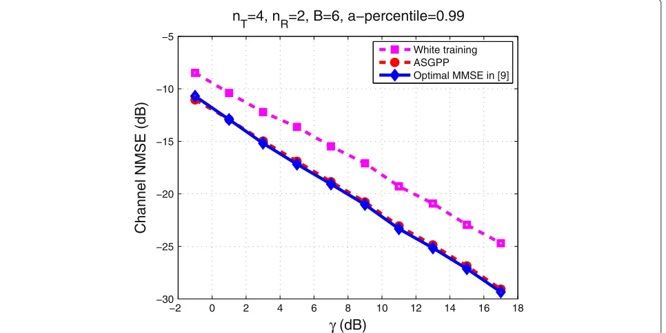
In Figure 1, the channel estimation NMSE performance versus the accuracy γ is presented for three different schemes. The scheme ‘ASGPP’ is the optimal Wiener filter together with the optimal guaranteed performance train-ing matrix described in Subsection 5.1. ‘Optimal MMSE’ is the scheme presented in [9], which solves the optimal training problem for thevectorizedMMSE, operating on vec(Y). This solution is a special case in the statement of Theorem 5 forIadm = I, i.e., IT = IandIR = I.
Finally, the scheme ‘White training’ corresponds to the use of the vectorized MMSE filter at the receiver, with a white training matrix, i.e., one having equal singular val-ues and arbitrary left and right singular matrices. This scheme is justified when the receiver knows the involved channel and noise statistics but does not want to sacri-fice bandwidth to feedback the optimal training matrix to the transmitter. This scheme is also justifiable in fast fading environments. In Figure 1, we assume thatRR =
SR, and we implement the corresponding optimal
train-ing design for each scheme. ASGPP is implemented first for a certain value of γ, and the rest of the schemes are forced to have the same training energy. The Opti-mal MMSE in [9] and ASGPP schemes have the best and almost identical MSE performance. This indicates that for the problem of training design with the classical chan-nel estimation MSE, the confidence ellipsoid relaxation of the chance constraint and the relaxation based on the Markov bound in Subsection 4.4 deliver almost identical performances. This verifies the validity of the approxi-mations in this paper for the classical channel estimation problem.
Figures 2 and 3 demonstrate the L-optimality average performance metricE{JW}versusγ. Figure 2 corresponds
to the L-optimality criterion based on MVU estimators and Figure 3 is based on MMSE estimators. In Figure 2, the scheme ‘MVU’ corresponds to the optimal training for channel estimation when the MVU estimator is used. This training is given by Theorem 4 forIadm =I, i.e.,IT =I
andIR = I. ‘MVU in Subsection 4.4’ is again the MVU
−2 0 2 4 6 8 10 12 14 16 18 −30
−25 −20 −15 −10 −5
γ (dB)
Channel NMSE (dB)
n
T=4, nR=2, B=6, a−percentile=0.99
White training ASGPP
Optimal MMSE in [9]
Figure 1Channel estimation NMSE based on Subsection 5.1 withRR=SR.nT=4,nR=2,B=6,a(%)=99.
confidence ellipsoid and Markov bound approximations are better than the optimal training for standard channel estimation. Therefore, for this problem, the application-oriented training design is superior compared to training designs with respect to the quality of the channel estimate. Figure 4 demonstrates the performance of optimal train-ing designs for the MMSE estimator in the context of
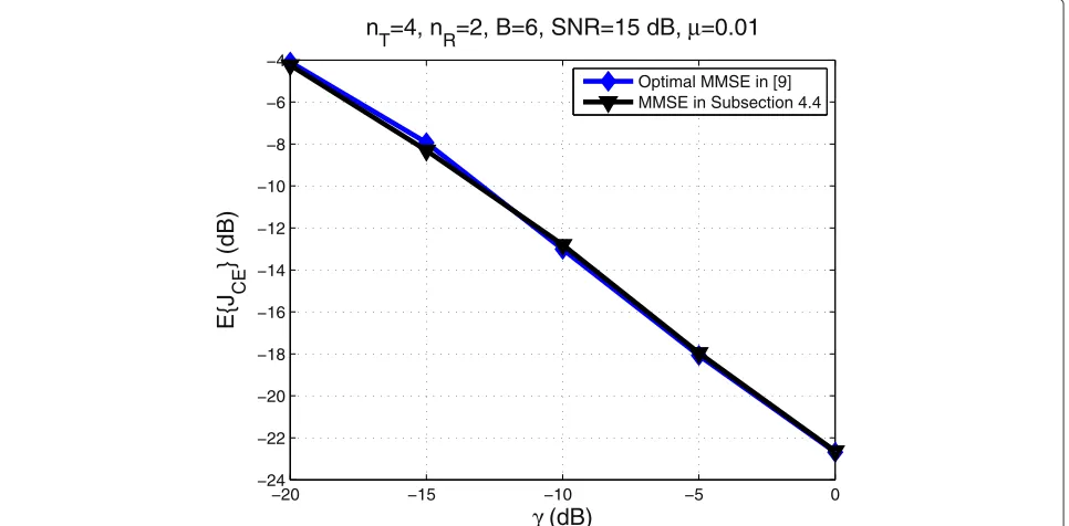
MMSE channel equalization. We assume thatRR = SR,
since the high SNR expressions forIadmin the context of MMSE channel equalization in Appendix 1 indicate that IT = Ifor this application and according to Theorem 5
the optimal training corresponds to the optimal training for channel estimation in [8]. We observe that the curves almost coincide. Moreover, it can be easily verified that for
−10 −5 0 5 10
−20 −15 −10 −5 0 5
γ (dB)
E{J
W
} (dB)
nT=6, nR=6, B=8, a−percentile=0.99
MVU ADGPP
MVU in Subsection 4.4
−10 −8 −6 −4 −2 0 −20
−15 −10 −5
γ (dB)
E{J
W
} (dB)
n
T=3, nR=3, B=4, a−percentile=0.99
Optimal MMSE in [9] ASGPP
MMSE in Subsection 4.4
Figure 3L-optimality criterion with arbitrary but positive semidefiniteW1,W2for the MMSE estimator withRR=SR.nT=3,nR=3, B=4,a(%)=99.
MMSE channel equalization with the MVU estimator, the optimal training designs given by Theorems 2 and 4 differ slightly only in the optimal power loading. These obser-vations essentially show that the optimal training designs for the MVU and MMSE estimators in the classical chan-nel estimation setup are nearly optimal for the application
of MMSE channel equalization. This relies on the fact that for this particular application, IT = Iin the high data
transmission SNR regime.
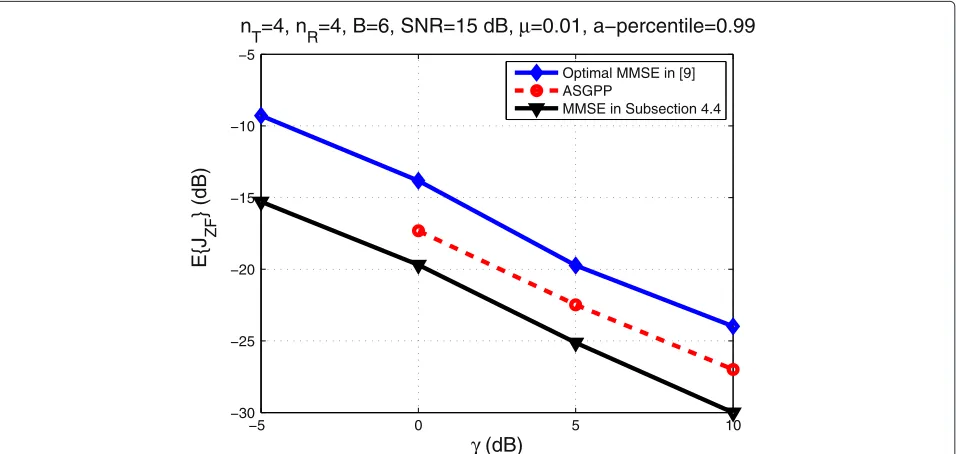
Figures 5 and 6 present the corresponding performances in the case of the ZF precoding. The descriptions of the schemes are as before. In Figure 6, we assume that
−20 −15 −10 −5 0
−24 −22 −20 −18 −16 −14 −12 −10 −8 −6 −4
γ (dB)
E{J
CE
} (dB)
n
T=4, nR=2, B=6, SNR=15 dB, μ=0.01
Optimal MMSE in [9] MMSE in Subsection 4.4
−10 −5 0 5 10 −25
−20 −15 −10 −5 0 5 10
γ (dB)
E{J
ZF
} (dB)
n
T=5, nR=5, B=7, SNR=15 dB, μ=0.01, a−percentile=0.99
MVU ADGPP
MVU in Subsection 4.4
Figure 5ZF precoding based on Subsection 5.4 for the MVU estimator.Iadmis based on a previous channel estimate.nT=5,nR=5, B=7, SNR=15 dB,a(%)=99,μ=0.01.
RR = SR. The superiority of the application-oriented
designs for the ZF precoding application is apparent in these plots. Here, IT = I and this is why the
opti-mal training for the channel estimate works less well in this application. Moreover, the ASGPP is plotted for γ ≥ 0 dB, since for γ ≤ −5 dB all the eigenvalues of
B=
cλmax(SRIR)IT −R−1T
+are equal to zero for this particular set of parameters defining Figure 6.
Figure 7 presents an outage plot in the context of the L-optimality criterion for the MVU estimator. We assume that γ = 1. We plot Pr{JW >1/γ} versus the
train-−5 0 5 10
−30 −25 −20 −15 −10 −5
γ (dB)
E{J
ZF
} (dB)
n
T=4, nR=4, B=6, SNR=15 dB, μ=0.01, a−percentile=0.99
Optimal MMSE in [9] ASGPP
MMSE in Subsection 4.4
Figure 6ZF precoding MSE based on Subsection 5.4 for the MMSE estimator withRR=SR.Iadmis based on a previous channel estimate.
0 5 10 15 20 25 30 35 10−3
10−2 10−1 100
Training Energy (dB)
Pr{J
W
>1/
γ
}
n
T=6, nR=6, B=8, γ=1
MVU ADGPP
MVU in Subsection 4.4
Figure 7Outage probability for the L-optimality criterion with the MVU estimator.nT=6,nR=6,B=8,γ=1. The accuracy parameter is γ =1.
ing power. This plot indirectly verifies that the confi-dence ellipsoid relaxation of the chance constraint given by the scheme ASGPP is not as tight as the Markov bound approximation given by the scheme MVU in Subsection 4.4.
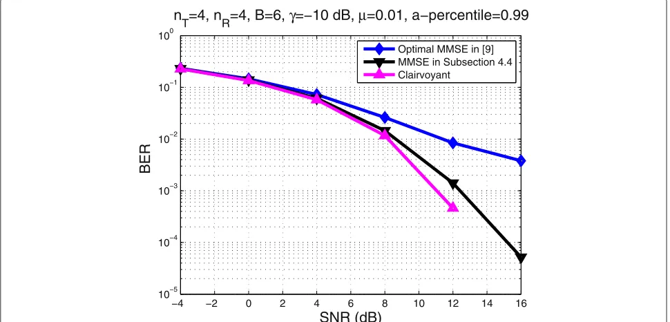
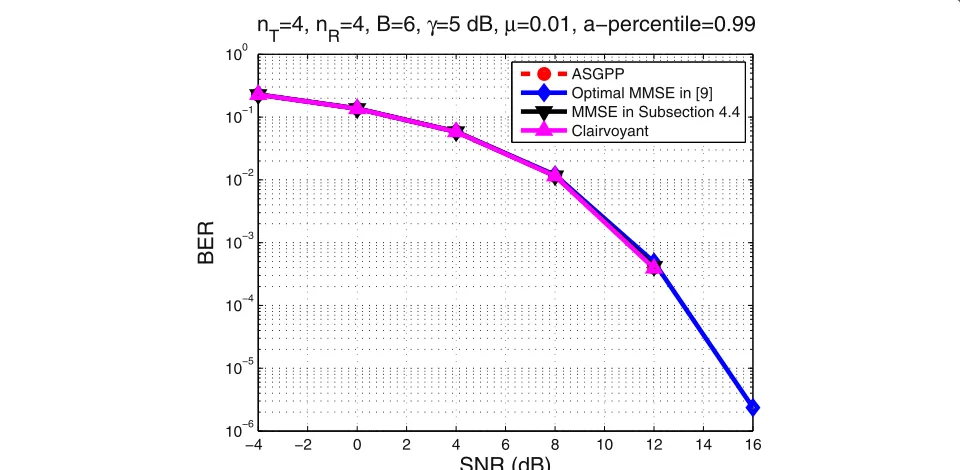
Finally, Figures 8 and 9 present the BER performance of the nearest neighbor rule applied to the signal estimates produced by the corresponding schemes in Figure 6. The used modulation is quadrature phase-shift keying (QPSK). The ‘Clairvoyant’ scheme corresponds to the ZF
−4 −2 0 2 4 6 8 10 12 14 16 10−5
10−4 10−3 10−2 10−1 100
SNR (dB)
BER
n
T=4, nR=4, B=6, γ=−10 dB, μ=0.01, a−percentile=0.99
Optimal MMSE in [9] MMSE in Subsection 4.4 Clairvoyant
−4 −2 0 2 4 6 8 10 12 14 16 10−6
10−5 10−4 10−3 10−2 10−1 100
SNR (dB)
BER
n
T
=4, n
R=4, B=6,
γ
=5 dB,
μ
=0.01, a−percentile=0.99
ASGPP
Optimal MMSE in [9] MMSE in Subsection 4.4 Clairvoyant
Figure 9BER performance using the signal estimates produced by the corresponding schemes in Figure 6 withRR=SRandγ=5dB. Iadmis based on a previous channel estimate.nT=4,nR=4,B=6,γ=5 dB,μ=0.01,a(%)=99.
precoder with perfect channel knowledge. The channel estimates have been obtained for γ=−10 and 0 dB, respectively. Even if the application-oriented estimates are not optimized for the BER performance metric, they lead to better performance than the Optimal MMSE scheme in [9] as is apparent in Figure 8. In Figure 9, the per-formances of all schemes approximately coincide. This is due to the fact that for γ =5 dB, all channel estimates are very good, thus leading to symbol MSE performance differences that do not translate to the corresponding BER performances for the nearest neighbor decision rule.
7 Conclusions
In this contribution, we have presented a quite general framework for MIMO training sequence design subject to flat and block fading, as well as spatially and tempo-rally correlated Gaussian noise. The main contribution has been to incorporate the objective of the channel estimation into the design. We have shown that by a suitable approximation ofJ(H, H), it is possible to solve this type of problem for several interesting applications such as standard MIMO channel estimation, L-optimality criterion, MMSE channel equalization, and ZF precod-ing. For these problems, we have numerically demon-strated the superiority of the schemes derived in this paper. Additionally, the proposed framework is valuable since it provides a universal way of posing different estimation-related problems in communication systems.
We have seen that it shows interesting promise for, e.g., ZF precoding, and it may yield even greater end performance gains in estimation problems related to communication systems, when approximations can be avoided, depending on the end performance metric at hand.
Endnotes
aThe word ‘dual’ in this paper defers from the
Lagrangian duality studied in the context of convex optimization theory (see [24] for more details on this type of duality).
bFor simplicity, we have assumed a zero-mean channel,
but it is straightforward to extend the results to Rician fading channels, similar to [9].
cWe set the subscriptQtoS
Qto highlight its temporal
nature and the fact that its size isB×B. The matrices with subscriptTin this paper share the common characteristic that they arenT×nT, while those with subscriptRarenR×nR.
dFor a Hermitian positive semidefinite matrix A, we
consider here thatA1/2is the matrix with the same eigen-vectors asAand eigenvalues as the square roots of the cor-responding eigenvalues of A. With this definition of the square root of a Hermitian positive semidefinite matrix, it is clear thatA1/2 = AH/2, leading toA = A1/2AH/2 = AH/2A1/2.
eFor easiness, we use the MATLAB notation in
Appendix 1
Approximating the performance measure for MMSE channel equalization
In order to obtain the approximating setDadm, let us first denote the integrand in the performance metric (33) by
J(ω;H,H)=tr(ejω;H, H)y(ω)H(ejω;H, H).
(37)
In addition, letdenote an equality in which only dom-inating terms with respect to ||H|| are retained. Then, using (32), we observe that
(ejω;H, H)=F(ejω;H+H)−F(ejω;H)
λxHH−y1−λ2xHHy−1(HHH+HHH)−y1
=λx
⎛ ⎜ ⎜ ⎝
I−λxHH−y1H
=Q
HH−y1−λxHH−y1HHH−y1
⎞ ⎟ ⎟ ⎠,
(38)
where we omitted the argumentωfor simplicity. Inserting (38) in (37) results in the approximation
J(ω;H,H)λ2xtrQHH−1y HQ
+λ2x
HH−1y HHH−1y HHH−1y H
−λxQHHy−1HHH−1y H
−λxHH−1y HH H−1y HQ . (39)
To rewrite this into a quadratic form in terms of vec(H), we use the facts that tr(AB) = tr(BA) = vecT(AT)vec(B) = vecH(AH)vec(B) and vec(ABC) =
(CT ⊗A)vec(B)for matricesA, B, andCof compatible dimensions. Hence, we can rewrite (39) as
J(ω;H,H)vecH(H)[λ2xQ2T⊗−1y ] vec(H)
+vecH(H)[λ 4x(HH−1y H)T⊗−1y HHH−1y ] vec(H)
−vecH(H)[λ 3x(y−1HQ)T⊗−1y H] vec(HH)
−vecH(HH)[λ3x(QHH−1y )T ⊗HH−1y ] vec(H). (40)
In the next step, we introduce the permutation matrix
defined such that vec(HT) =vec(H) for everyHto rewrite (40) as
J(ω;H,H)vecH(H)[λ2xQ2T⊗−1y ] vec(H)
+vecH(H)[λ4x(HH−1y H)T⊗−1y HHH−1y ] vec(H)
−vecH(H)[λ3x(−1y HQ)T⊗−1y H]vec(H∗)
−vecH(H∗)T[λ3x(QHH−1y )T⊗HH−1y ] vec(H). (41)
We have now obtained a quadratic form. Note indeed that the last two terms are just complex conjugates of each other and thus we can write them as two times their real part.
High SNR analysis
In order to obtain a simpler expression forIadm, we will assume high SNR in the data transmission phase. We consider the practically relevant case where rank(H) = min(nT,nnnR). Depending on the rank of the channel
matrixH, we will have three different cases:
Case1.rank(H)=nR<nT
Under this assumption, it can be shown that both the first and the second terms on the right hand side of (41) con-tribute to Iadm. We have Q → H⊥H and λx−1y →
(HHH)−1for high SNR. Here, and in what follows, we use
X=XX†to denote the orthogonal projection matrix on the range space ofXand⊥X=I−Xto denote the pro-jection on the nullspace ofXH. Moreover,λxHH−1y H→ HH andλ2x−1y HHH−1y →(HHH)−1for high SNR. As ⊥
HH+HH=I, summing the contributions from the first
two terms in (41) finally gives the high SNR approximation
Iadm=λxI⊗(HHH)−1. (42)
Case2.rank(H)=nR=nT
For the non-singular channel case, the second term on the right hand side of (41) dominates. Here, we have λxHH−1y H → Iandλ2x−1y HHH−1y → (HHH)−1for
high SNR. Clearly, this results in the same expression for Iadmas in Case 1, namely
Iadm=λxI⊗(HHH)−1. (43)
Case3.rank(H)=nT<nR
λxHH−1y H → Iandλ2x−1y HHH−1y → −1
/2
n [−1n /2
HHH−1n /2]†−1n /2for high SNR. Using these
approxi-mations finally gives the high SNR approximation
Iadm=λxI⊗
For the low SNR regime, we do not need to differentiate our analysis for the casesnT ≥nRandnT < nRbecause
now y → n. It can be shown that the first term on
the right hand side of (41) dominates, that is, the term involving
For the proof of Theorem 1, we require some prelimi-nary results. Lemmas 1 and 2 will be used to establish the uniqueness part of Theorem 1, and Lemma 3 is an exten-sion of a standard result in majorization theory, which is used in the main part of the proof.
Lemma 1. LetD∈Rn×nbe a diagonal matrix with
ele-from which we have, by the orthonormality of the columns ofU, that
Proof. The idea is similar to the proof of Lemma 1. We proceed by induction on the ith column of V. For the first column ofV we have, by the orthonormality of the columns ofUandV, that
|u1,1|2+ If now the assertion holds for columns 1 tok, the orthog-onality of the columns ofUimplies thatui,k+1 = 0 for
where {(A)[i,i]}i=1,...,n denotes the ordered set {(A)
1,1,. . .,(A)n,n} sorted in descending order. Since
{(A)[i,i]}i=1,...,n ismajorizedby{a1,n. . .,an}and thebi’s
are distinct, we can use ([34], Theorem 3.A.2) to show that
n diagonal, but this follows from Lemma 1.
Proof of Theorem 1
First, we simplify the expressions in (21). Using the eigen-decompositions in (23) ofAandB, we see that
PA−1PH B ⇔ PUAD−1A UHAPH UBDBUHB
⇔ UHBPUAD−1A UHAPHUBDB.
Now, defineP¯ =UHBPUAD−1A /2and observe that
tr(PPH)=tr(UBPD¯ −AH/2UHA)(UBPD¯ −AH/2UHA)H
=tr(UBPD¯ −1A P¯HUBH)=tr(P¯HPD¯ −1A ).
Therefore, (21) is equivalent to
minimize
To further simplify our problem, consider the singular value decompositionP¯ = UVH, whereU ∈ Cn×nand
observe that (46) is equivalent to
minimize
With this problem formulation, it follows (from Sylvester’s law of inertia [35]) that we needm≥rank(DB)
to achieve feasibility in the constraint (i.e., having at least
as many non-zero singular values ofas non-zero eigen-values in DB). This corresponds to the condition N ≥
rank(B)in the theorem.
Now, we will show thatUandVcan be taken to be the identity matrices. Using Lemma 3, the cost function can be lower bounded as
whereλj(·)denotes thejth largest eigenvalue. The equality
is achieved ifV = I, and observe that we can selectVin this manner without affecting the constraint.
To show thatUcan also be taken as the identity matrix, notice that the cost function in (47) does not depend on U, while the constraint implies (by looking at the diagonal elements of the inequality and recalling thatUis unitary) that
σi2≥(DB)i,i, i=1,. . .,m, (49)
requiringm≥rank(DB). Suppose thatU¯ and¯ minimize
the cost. Then, we can replaceU¯ byIand satisfy the con-straint, without affecting the cost in (48). This means that there exists an optimal solution withU=I.
WithU = IandV = I, the problem (47) is equivalent
It is easy to see that the optimal solution for this problem isσiopt=(DB)i,i,i=1,. . .,m. By creating an optimal,
denoted asopt, with the singular valuesσ1opt,. . .,σmopt,
we achieve an optimal solution
Popt=UBPD¯ A1/2UHA=UBoptD1A/2UAH =UBDPUHA
withDPas stated in the theorem.
Finally, we will show how to characterize all optimal solutions for the case whenAandBhave distinct non-zero eigenvalues (thus, m = n). The optimal solutions need to give equality in (48) and thus Lemma 3 gives that VHVH is diagonal and equal toH. Lemma 1 then
establishes that the firstncolumns ofUare of the form
where|ui,i| =1 fori=1,. . .,n. SinceUhas to be unitary
and its lastN−n+1 columns play no role inP¯(due to the form of ), we can take them as [0n,N−m+1 IN−m+1]T without loss of generality.
Summarizing, an optimal solution is given by (23). When AandB have distinct eigenvalues,V and Ucan only multiply the columns ofUAandUB, respectively, by
complex scalars of unit magnitude.
Appendix 3
Proof of Theorems 2 and 3
Before proving Theorems 2 and 3, a lemma will be given that characterizes equivalences between different sets of feasible training matricesP.
Lemma 4. LetB ∈ Cn×n andC ∈ Cm×m be Hermi-tian matrices and f : Cn×N →Cn×nbe such that f(P) =
f(P)H. Then, the following sets are equivalent
{P|f(P)⊗IB⊗C} = {P|f(P)λmax(C)B}. (50)
Proof. The equivalence will be proved by showing that the left hand side (LHS) is a subset of right hand side (RHS) andvice versa. First, assume thatf(P)λmax(C)B, then
f(P)⊗Iλmax(C)B⊗I
=(B⊗λmax(C)I)(B⊗C).
(51)
Hence, RHS⊆LHS.
Next, assume thatf(P)⊗IB⊗C, but for the purpose of contradiction thatf(P)λmax(C)B. Then, there exists a vectorxsuch thatxH(f(P)−λmax(C)B)x<0. Letvbe an eigenvector ofCthat corresponds toλmax(C)and define y=x⊗v. Then,
y(f(P)⊗I−B⊗C)y
=(xHf(P)x)v2−(xHBx)(vHCv)
=xH(f(P)−λmax(C)B)xv2<0
(52)
which is a contradiction. Hence, LHS⊆RHS.
Proof of Theorem 2
Rewrite the constraint as
PH(STQ⊗SR)−1PcITT⊗IR
⇔ (PS−1Q PH)T⊗S−1R cITT⊗IR
⇔ (PS−1Q PH)⊗IcIT⊗SRIR.
(53)
Letf(P) = PS−1Q PH. Then, Lemma 4 gives that the set of feasiblePis equivalent to the set of feasiblePwith the constraint
(PS−1Q PH)cλmax(SRIR)IT. (54)
Proof of Theorem 3
In the case thatRR= SR, the constraint can be rewritten
as
(PS−1Q PH+R−1T )T⊗IcITT⊗SRIR. (55)
Withf(P) =PS−1Q PH+R−1T , Lemma 4 can be applied to achieve the equivalent constraint
PS−1Q PH+R−1T cλmax(SRIR)IT
⇔ PS−1Q PH cλmax(SRIR)IT−R−1T
⇔ PS−1Q PH [cλmax(SRIR)IT−R−1T ]+
(56)
where the last equality follows from the fact that the left hand side is positive semidefinite.
In the case that R−1R = IR, the constraint can be
rewritten as
(PS−1Q PH)T⊗S−1R (cIT−RT)T ⊗IR
⇔ (PS−1Q PH)T⊗S−1R [cIT −RT]T+⊗IR.
(57)
Observe that this expression is identical to the constraint in (24), except that the positive semidefiniteIT has been
replaced by [cIT −RT]+. Thus, the equivalence follows
directly from Theorem 2.
In the caseR−1T =IT, the constraint can be rewritten as
(PS−1Q PH)T⊗S−1R ITT⊗(cIR−RR)
⇔ (PS−1Q PH)T⊗S−1R ITT⊗[cIR−RR]+.
(58)
As in the previous case, the equivalence follows directly from Theorem 2.
Appendix 4 Proof of Theorem 4
Our basic assumption is thatIT,IRare both Hermitian
matrices, which is encountered in the applications pre-sented in this paper. Denoting by P the matrixPT and using the fact thatdIadm =
I
T⊗IR
1/2I
T⊗IR
1/2 , it can be seen that our optimization problem takes the following form
minimize P∈CB×nT
J(H)
s.t. tr(PPH)≤P, (59)
whereJ(H)=EH
J(H,H)is given by the expression
tr
I−1/2
T P H
S−Q1PI−1T/2⊗I−1R /2S−1R I−1R /2
−1
=tr
I−1/2
T P H
S−Q1PI−1T/2
−1 ⊗I1/2
R SRI1R/2