MSNS: mobile sensor network simulator for area coverage and obstacle avoidance based on GML

R E S E A R C H

Open Access

MSNS: mobile sensor network simulator for area

coverage and obstacle avoidance based on GML

Young-Sik Jeong

, Youn-Hee Han

, James J Park

and SooYoung Lee

Abstract

A mobile sensor network is a distributed collection of sensors, each of which has sensing, computation,

communication, and locomotion capabilities. In particular, locomotion facilitates the ability to self-deployment. In such a network of self-deployable mobile sensors, it is difficult to evaluate the effectiveness of mobile sensor network deployment in a given target area because we cannot predict the coverage rate for the target area. The coverage rate will be changed due to the number of sensor required in the target area, connectivity degree to be maintained and unknown obstacles. In this article, we develop mobile sensor network simulator (MSNS) in order to visualize (1) coverage secured by mobile sensors and (2) avoidance of obstacle objects (building, road and wall, and so on) on the real map drawn by GML (Geography Markup Language). From a user, MSNS receives the number of mobile sensor nodes, connectivity degree, sensor node’s sensing range, communication range, and supersonic wave range. And then it visualizes the location information of sensor nodes, connectivity degree, and sensing coverage, all of which change with simulation time. Thereby we can estimate how many nodes are required in a given target area, and also calculate coverage rate of the target area in advance to the real deployment of mobile sensors.

Keywords:mobile sensor network, visual coverage, connectivity, potential field

1. Introduction

Mobile sensor network is made up of group/groups of small low-power sensor nodes that can sense specific situations or collect information, and then transmit that information to sink nodes using wireless ad hoc com-munication. In general, mobile sensor network, which is very useful for the target fields to be difficult to access, should be constructed by using mobile sensor nodes with sensing, computation, communicating, and loco-motion capabilities. In particular, locoloco-motion facilitates the ability to self-deployment. Several nodes with var-ious kinds of sensors for sound, heat, magnetic field, and infrared ray are randomly scattered in a target area. These sensors move, voluntarily avoiding obstacles and other nodes, establish sensing coverage and configure their communication network [1]. And after sensing the information, the sensor transmits such information as sensing information to the sink node through routing

path. The sink node sends the sensing information to middleware or server before processing it for applica-tion. This technology is used in various fields such as medical care, transportation, military, environment, and disaster prevention.

Coverage and connectivity are ones of critical factors to establishing mobile sensor network [2,3]. The coverage means the area in which sensing by sensor nodes is possi-ble. The connectivity means how many sensors are con-nected to cover the entire area for sensing or detecting, and deliver any sensing information to the sink node. The mobile sensor network, established in a given target area where terrain status is unknown, is required to maximize sensing coverage with mobile sensors and maintain the connectivity as much as a network administrator requires.

When self-deployable mobile sensors are deployed in a given target area to be required for monitoring, sensing, and detecting; however, it is difficult to predict how many sensors are needed in the target area and how much connectivity the sensor network have, which pre-vents guaranteeing the effectiveness of network deployment.

* Correspondence: [email protected]

3

Department of Computer Science and Engineering, Seoul National University of Science and Technology, Seoul, South Korea Full list of author information is available at the end of the article

In this article, a new simulator, mobile sensor network simulator (MSNS), is designed and implemented. From a user, MSNS receives the information on the number of mobile sensor nodes, connectivity degree, sensor node’s sensing range, communication range, and super-sonic wave range. In the simulator, the target area is set when a user designates a random area where obstacles are set by using GML (Geography Markup Language). A number of sensors input by the user are randomly deployed in the target area, and they move to avoid obstacles while maximizing the coverage in the target area and maintaining the given connectivity. MSNS visualizes the location information of sensor nodes, con-nectivity degree, and sensing coverage, all of which change with simulation-time. It can be used to find out the coverage rate of the target area secured by the given mobile sensors. Thereby we can estimate how many nodes are required in a given target area, and also calcu-late coverage rate of the target area in advance to the real deployment of mobile sensors.

This article is organized as follows. Section 2 presents the existing simulators related to this research, moving method of sensor in the mobile sensor network, and the results of studies on coverage and connectivity of sen-sors. Section 3 explains the GML-based obstacle setting technique, which is the one of keys to MSNS, and the MSNS coverage algorithm to be used for self-deploy-ment of mobile sensors. Section 4 shows the design and implementation of MSNS based on the technique sug-gested in Section 3. Section 5 presents the evaluation of MSNS’s functions and the results of coverage algo-rithm’s performance. Finally, Section 6 suggests the con-clusions and discussion on the future researches.

2. Related studies

Related studies are explained in the two perspectives: development of ubiquitous sensor network (USN) simu-lator and coverage and connectivity of mobile sensor network. First, existing USN simulators focus on the verification of packets, protocol, and the network. Through such a method, a simulation can be run on the network lifetime on some simulators. TOSSIM, an open source TinyOS-based simulator from UC Berkeley, can simulate Mica2 series simulation from CrossBow. Main features are packet loss calculation and CRC sensing. However, it can only work with Mica2 series. GloMo-Sim, a PARSEC (C-based parallel simulation language)-based discrete event simulator, is a simulation environ-ment for wireless mobile network. Like OSI 7-hierarchi-cal model, GloMoSim is composed of number of layers. It monitors packet transmission status, and verifies net-work model or transmission scenario; however, it cannot work as sensor network. GloMoSim’s next version, QualNet is a massive wireless network simulator. It uses

IEEE 802.11 MAC and Physical Layer standard, and like GloMoSim it has several layers. When modules for layer are developed by different designers, the scenarios and models are being tested. Packet flow statistics can be checked through automatically collected data from each layer. Features for sensor network are designed as well; nevertheless, visualization of sensed objects. NS2 is most widely used network simulator, and many wired and wireless network simulators have been developed based on this system. It is a discrete event simulator, it can simulate various network protocols; however, it has too many nodes and is difficult to adapt to complex massive system. It also has too much unnecessary interdepen-dency. J-Sim is a JAVA-based open source WSN simula-tor. Each component uses autonomous component architecture, and imitates software with IC chips. It is designed in loosely coupled structure so that is can sup-port plug & play. It can calculate memory usage, num-ber of events, and running time according to size of given network. It also simulates transmission status of transmitted event from target node being transmitted to sink nodes in packet form. Nevertheless J-Sim is difficult to visualize target node sensor. SWANS is an expansion of Jist, a PARSEC-based scattered event simulator. It is an open source simulator, and compared to NS2 or Glo-MoSim, it can carry out massive network simulation; nevertheless, like other simulators it can only carry out protocol verification [4,5].

Second, suggestion was made on the algorithm that enabled maximization of the area that could be covered in the mobile sensor network where potential field was applied so that initial sensors moved voluntarily [6]. On the assumption that there was a repulsive force between sensors or sensor and obstacle, such force was used to have sensors dispersed evenly on the network and to ensure that friction force, opposite to the repulsive force, was applied so that sensors reached the static equilibrium without any movement. The algorithm sug-gested in this article basically utilizes what is sugsug-gested in [6]. However, the difference is that sensors are induced in the way that local coverage is maximized rather than sensors simply being spread.

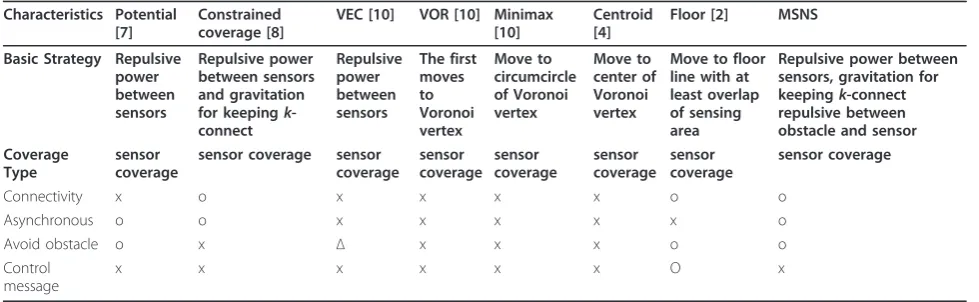
Minimax method. In each method, information on loca-tion of neighboring sensors is acquired for each step, Voronoi polygon is drawn, and then, sensors move in the way to minimize the area where coverage is not secured in such polygon. Among the three methods, the VOR shows that sensors move toward the most distant vertex of the Voronoi polygon while the Minimax shows that sensors move toward the circumcenter of the Voro-noi polygon.

As the case with [7], the previous study [8] also solved the problem on self-deployment of sensors based on the Voronoi diagram. The study [8] suggested the method that sensors utilized information on location of neigh-boring sensors for each step to configure the Voronoi polygon before moving toward the centroid of the poly-gon. The centroid of the Voronoi polygon is the mean position of all points inside the Voronoi polygon. In other words, the centroid is the point that a random sensor has the smallest value in the sum of variance of distance up to each vertex of the Voronoi polygon. If sensor moves to this point, the sensor is placed in the best position to cover the Voronoi polygon [9].

Lastly, the previous study [10] suggested that sensors should be moved in consideration of not only minimiza-tion of moving distance, but also remaining energy because self-deployment of sensors in itself consumes a great deal of energy. The study presented three algo-rithms that ensured the balanced deployment of the entire network by changing the degree of movement in consideration of local density of each sensor (number of neighboring sensors) and remaining energy. Table 1 shows comparison of the characteristics of the existing methods and the MSNS.

3. Mechanism of field and mobile sensor moving 3.1. Field establishment

Establishment of the target area is one of the important issues to execute MSNS. When mobile sensor network

is established for various applications, the number of terrains is as many as the number of applications. Therefore, MSNS uses the method of establishing field where mobile sensor network is to be formed and based on such terrain, selecting target area that requires observation.

MSNS uses the GML [11-14] to establish field that includes obstacles. Since the GML is the standard for geospatial data, it has the high compatibility and is con-venient for configuring field. And as the GML contains the coordinate information, it is possible to utilize the information to calculate the actual coordinate informa-tion of mobile sensors that estimate the locainforma-tions of each other based on the relative coordinates. In the GML, factors that can be obstacles such as building are written mostly with polygon. Therefore, MSNS sets the polygon of the GML as an obstacle and processes it.

3.2. Coverage of MSNS

Another important issue to implement the MSNS is the moving technique for mobile sensors. The mobile sen-sors are required to maintain a given connectivity, avoid obstacles, and maximize coverage in the target area. Therefore, this article suggests the coverage method that adds the obstacle avoidance method to the constrained coverage method that maximizes coverage while main-taining the given connectivity [8,15].

The method has preconditions as follows. First, the method is based on the binary model that mobile sensors sense the target within the sensing range at the rate of 100% but cannot sense the target out of the sensing range. Second, all of the mobile sensors have the equal sensing distance (Rs) and the equal communication

dis-tance (Rc). Third, mobile sensors have the method to

determine their location in order to calculate virtual force. Lastly, the method does not take into consideration distortion of sensing range and communication range of mobile sensors due to waves reflected by obstacles.

Table 1 Moving method of mobile sensors

Characteristics Potential [7]

Constrained coverage [8]

VEC [10] VOR [10] Minimax [10]

Based on the potential filed method [6] frequently used for movement of robot in mobile robotics, the three virtual forces such as Fcover, Fdegree, andFobstacle

are used for movement of mobile sensors. In order to maximize coverage, mobile sensors are basically required to have a certain distance from one another to ensure that their sensing range is not overlapped with others.

Fcover is the force with which mobile sensors push

against one another to maximize the sensing range in the target area.Fcover(i, j) means the force that the

sen-sor S_i takes from the neighboring sensor S_j during the unit time, which is expressed in Equation (1).

Fcover(i,j) = −

In Equation (1), xi and xj represent the locations of

sensorssiandsj whileΔijmeans the Euclidian distance

of sensors si and sj. And Ccover is the constant that

means force of field.

In mobile sensor network, the mobile sensor that senses the information that requires observation in the target area uses the connection between mobile sensors in order to send the collected information to sink node. In this case, if a parent sensor on the path that is used to send information to one sink node loses connection for reasons such as failure or malfunction, a child sensor uses an alternative sensor that exists within its commu-nication distance to form a new path. This local connec-tivity influences the entire connecconnec-tivity [3]. In addition, sensors are required to maintain communication with a certain number or more of their neighboring sensors in order to deploy numerous mobile sensors in the target area with some sensors in the active state and others in the sleep state, which aims at increasing lifetime of the network [16].

Fdegreeis the force that is exerted by mobile sensors to

keep the number of given neighboring sensors at the degreeK. Figure 1 shows deployment of sensor nodes in case ofK = 3. If the number of neighboring sensors is larger thanKthat should be kept,Fdegree does not take

place, and sensors become distant from each other due to Fcover. The sensors become more distant gradually to

maximize coverage, and if the number of neighboring sensors is equal to a given degreeK,Fdegreetakes place.

As a result, a sensor draws its neighboring sensors to keep the number of neighboring sensors at the given degreeK.Fdegree(i, j) means the force that the sensorSi

takes from its neighboring sensor Sj during the unit

time, which can be expressed in Equation (2).

Fdegreei,j=

if count of neighbor sensor=k

otherwise (2)

whereRcmeans communication distance whileCdegree

is the constant that means force of field. Mobile sensors in MSNS are required to maximize coverage, maintain the given connectivity and avoid obstacles. To this effect, this article definesFobstacle.

It is assumed that mobile sensors are equipped with 16 supersonic wave sensors (sender = 8, receiver = 8) in order to obtain Fobstacle. Figure 2 shows that supersonic

wave sensors locate obstacles. It is assumed that if supersonic wave distance (Rw) is determined and a

sen-sor detects obstacle within the distance ofRw, the sensor

with sensing range ofRwis located in the point that is

two times of the distance between the obstacle and the sensor. Fobstacle is calculated in the same way asFcoverin

order to maximize the range ofRw. Fobstacle(i, k) takes

place between the sensor node S_i and the obstacleo_k during the unit time, which can be expressed in Equa-tion (3).

whereok is the location of obstacle whileΔikis the

Euclidian distance between mobile sensor and obstacle, andCobstacleis the constant that is caused by obstacle.

(a) (b)

Figure 1 Deployment of sensors withK= 3.(a)Number of neighbor sensors >K;(b)number of neighbor sensors =K.

Fcover, Fdegree, and Fobstacleare used to calculate the

total virtual force Fthat mobile sensor Si takes during

the unit time, which is expressed in Equation (4).

F =

neighbors i(Fcover(i,j) +Fdegree(i,k)) +

founded obstacles kFobstacle(i,k) (4)

Mobile sensors continue to move at a constant speed if only Fcover, Fdegree, and Fobstacleare considered. The

virtual force Fdamper, which needs to stop sensors from

continuous movement, is defined as in Equation (5).

Fdamper =σ·vcurrent (5)

where sis damper constant while vcurrent is moving

speed of the current sensor.Fdamper is calculated based

on the damper constant and the moving speed of the current node as shown above. For application of Fcover, Fdegree, and Fobstacle, it is required to calculate Ccover, Cdegree, and Cobstaclethat are used for calculating each

force. Mobile sensors push against each other to maxi-mize coverage. And when the distance between them is 2Rs, the coverage becomes the highest. In other words,

when the distance between the two sensors is 2Rs,Fcover

does not take place between them, which is expressed in Equation (6). AndCcovercan be calculated.

Fcover−Fdamper= 0, whereij= 2Rs (6)

In a similar way, when the distance between obstacle and sensor isRs,Fobstacle does not take place to sensor,

which is expressed in Equation (7). AndCobstaclecan be

calculated.

Fobstacle−Fdamper= 0, whereij=Rs (7)

Sensors move due toFcover, Fdegree, and Fobstacle. And

there exists a moment when such forces reach the static equilibrium and the forces become zero (Equation 8).

Fcover+Fdegree+Fobstacle−Fdamper= 0, where,ij=μ·Rc (8)

In this case,μis a safety factor, and the range of value is 0 <μ< 1. If the value becomes close to 1, sensors are read-ily disconnected. This equation is used to calculateCdegree.

The calculated forceFthat one node takes per unit time can be used to calculate acceleration of mobile sen-sor and to calculate speed by using the acceleration value. And lastly, it is possible to calculate the next

location that sensor moves to (Equations 9-11). The cov-erage technique algorithm in MSNS is shown as follows.

Algorithm 1. MSNS coverage algorithm

1: While(MNS is playing)

2: get neighbor nodes of current node; 3: foreach neighbor nodedo

4: get Fcover& Fobstacle;

5: end for

6: if# of neighbor node < = K then

7: foreach neighbor nodedo

8: get Fdegree;

9: end for

10: end if

11: sum virtual force F; 12: calculate acceleration; 13: calculate velocity; 14: calculate next location;

15: ifnext location is contained in obstacle or out-side of target areathen

16: next location sets current location; 17: end if

18: end while

4. Design of MSNS 4.1. MSNS architecture

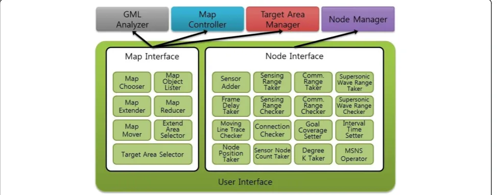
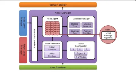
MSNS consists of user interface, GML analyzer, map layer manager, map controller, node manager, target area manager, and viewer. The overall structure of the MSNS is shown in Figure 3.

The user interface provides interface where users can enter set values necessary to start the MSNS. After the GML analyzer makes analysis of GML document, it cre-ates map objects before sending them to the map layer manager. The map layer manager plays a role in mana-ging map objects provided by the GML analyzer. And it also has control function related to map invoked by user interface. The map controller has the function of magnification, reduction, enlargement of area, and movement of the map information delivered to the map layer manager. The node manager applies sensor setting information entered in user interface to sensors, and creates and operates the obstacles defined in the map layer manager, the target area defined in the target area manager, and interactive sensors. The target area man-ager sets and manages the target area that requires detection and sensing in the field set by the GML docu-ment. The viewer visualizes map objects of the map layer manager and mobile sensors of the node manager.

4.2. Function of MSNS components 4.2.1. User interface

The map interface consists of seven modules as fol-lows: map chooser, which provides function of import-ing GML document to set the field where mobile sensor network is established; map lister, which visualizes the map, which is set up in MSNS, by object such as road or building; map extender, which magnifies the map; map reducer, which reduces the map; map mover, which moves the map to the desired place; extend area selector, which selects a specific area in the map and magnifies it; and target area selector, which selects the target area that requires detection and monitoring.

All of the functions set up by the map interface are delivered to the GML analyzer, the map controller, and the target area manager. Some of them can be used even after MSNS started deployment of mobile sensors. The node interface is composed of 16 modules. They include sensor adder, which adds mobile sensor to obtain desired coverage while MSNS is in operation; sensing range taker, which receives input of sensing range of sensor; communication range taker, which receives input of communication range of sensor; super-sonic wave range taker, which gets input of supersuper-sonic Figure 3Overall architecture of MSNS.

wave range of sensor to determine the location and dis-tance of obstacle; frame delay taker, which gets input of the value for MSNS to adjust moving speed of sensor; sensing range checker, which provides the visualization information on sensing range of sensor; communication range checker, which provides communication range of sensor; supersonic wave range checker, which delivers supersonic wave range of sensor; moving line trace checker, which traces the distance in which mobile sen-sors moved; connection checker, which checks connec-tivity between mobile sensors; goal coverage setter, which stops operation of the MSNS when mobile sen-sors reach the desired coverage; interval time setter, which sets the time to pause operation of MSNS at a certain time interval; node position taker, which sets the method of deployment of mobile sensors in the begin-ning; sensor node count taker, which receives input of the number of sensors that will be spread in the target area of MSNS; degree Ktaker, which determines con-nectivity degree that sensors are required to maintain; and MSNS operator, which controls operation of MSNS. All of functions of node interface also can be changed while MSNS is in operation.

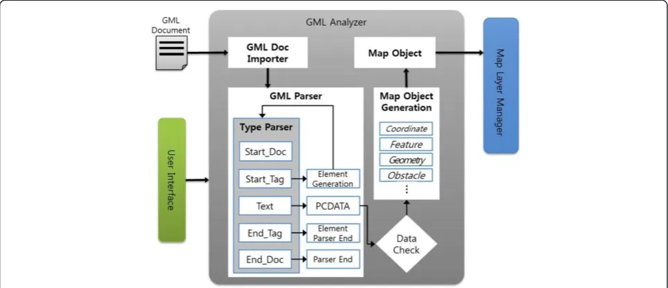
4.2.2. GML analyzer

Obstacle avoidance by using the GML in MSNS has the important meaning in the three perspectives. First of all, it is possible to simplify and visualize complex objects in the real world by using GML document. And it is easy to set obstacles because objects that can be obstacles in the GML such as building are configured in polygon. Lastly, the GML has the coordinate in the real world so that it is possible to take advantage of information on location of mobile sensor. The diagram of GML analyzer module is shown in Figure 5.

If the function to add a map through user interface is invoked, the GML document importer fetches GML document. The GML parser performs parsing of the GML document invoked by the GML document impor-ter to extract map objects. The extracted map objects contain coordinate information, features, shape informa-tion, and information to determine whether or not such objects are obstacles. The map objects created by the map GML parser are delivered to the map layer manager.

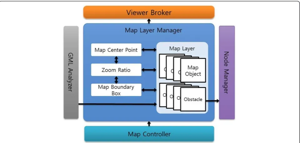
4.2.3. Map layer manager

The overall diagram shows the relation between the map layer manager and other major modules of the MSNS in Figure 6. The map objects that come from the GML analyzer are transmitted to the map layer. The map layer distinguishes map objects from obstacles after examining whether or not the map objects are config-ured in polygon. Afterward, the obstacles are sent to the node manager. When the map objects and the obstacles are set up, the map layer manager calculates the bound-ary box of the map and sets the zoon ratio at 1.0. And it sets the map center point at the dead center point of the map. If the setting is completed this way, the map center point, the zoom ratio and the map boundary box are changed by the map controller, and the map is dis-played on the MSNS through viewer broker.

4.2.4. Map controller

The map controller receives order of controlling the GML map and sets value to ensure that the map layer manager displays the map in the MSNS, following the request by user. The map center point setter sets value of the map’s center in the map layer manager when the map is magnified/reduced and when the area of the map in interest is shifted. The zoom ratio configurator

sets the zoom ratio in the map layer manager when the map is magnified/reduced. The full extender is used when the magnified/reduced/shifted map is drawn again to the entire area. The overall diagram of map controller is shown in Figure 7.

4.2.5. Node manager

In Figure 8, we show the detailed structure of node manager. Node configurator saves the information on sensing range, communication range, supersonic wave range, degree of connectivity, and the number of sensors to be deployed. The saved values are applied in batch when sensors are created by node generator. The super-sonic wave range is used to determine the location of obstacle in the target field where the sensor status is unknown. The node generator creates and manages the given number of sensors.

Initial location of the node generator determines if sensors start moving from the corner of the given target area, from the center, or from a random position. In addition, based on the initial position, mobile sensors determine the location for them to be deployed within the initial location of the target area. Node agent man-ages mobile sensors and ensures that sensors move, avoiding obstacles in the target area based on the cover-age algorithm suggested in Section 3, maintaining the degree Kand maximizing the coverage. If force, which was generated by sensor to find the results that the sen-sors in MSNS moved to cover a proper target area, is equal to or less than a critical value, the node agent stops MSNS from operating. Interaction interface refers to the target area in the target area manager and refers to obstacles in the map layer manager. The initial loca-tion of sensors in the node generator is set outside of obstacles and outside of polygon. When sensors in the node agent move, they avoid obstacles in the target area. Finally, statistics manager calculates information on mobile sensors observed by mobile agent. Elapsed time means unit time during which sensors move. Moving distance means the total distance that sensors move from their initially deployed position to the current position. Coverage rate provides information in percen-tage on the degree that mobile sensors cover the target area. Average neighbor means the average number of neighboring sensors out of the entire sensors.

4.2.6. Target area manager and viewer

The internal module diagram of target area manager and viewer are shown in Figure 9. The target area Figure 6Relationship map layer manager with other modules.

manager sets the target area in the mobile sensor net-work field. When a user drags the mouse to set the tar-get area that requires observation, the manager saves and manages the coordinate. And it sends the informa-tion on the target area to the node manager to ensure that sensors are created and operated within the target area. Then, the information is sent to viewer broker in order to visualize the target area in MSNS.

Coordinate system manager of the viewer replaces tar-get area of the tartar-get area manager and sensor of the node manager with MSNS screen coordinate based on the map coordinate that is set in the map layer manager. When map object is set by the map layer manager, map coordinate system is set by the boundary box. Screen coordinate system is set according to the size of view panel. If the screen coordinate system and the map coordinate system are set, the number of coordinate converters is calculated for conversion of the two sys-tems, which enables a free conversion of MSNS screen coordinate and the GML map coordinate. The coordi-nate converter changes the screen coordicoordi-nate to the map coordinate when a user sets the target area in the mobile sensor network field. And it changes the map coordinate to the screen coordinate when the map, the target area and the sensors are visualized in MSNS.

5. Implementation of MSNS

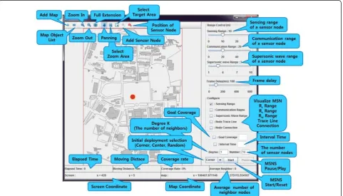
Figure 10 shows the initial screen and each control function of MSNS. Components of MSNS are as follows: toolbar; configuration panel, which has internal

properties of sensor and provides information such as sensing coverage; status panel, which shows various information when MSNS is in operation; and viewer, which provides the GML coordinate information and status information of sensors. The toolbar consists of the add button to import GML document in order to configure the field of mobile sensor network, the map object lister button to classify the map provided by the GML document according to object, the zoom in button to magnify the map, the zoom out button to reduce the map, the full extension button to provide the map con-trolled by magnification/reduction/movement, the select zoom area button to select and expand a specific area on the map, the select target area button to set the tar-get area on the map, the add sensor node button to add mobile sensor to ensure that the target area reaches the static equilibrium in the desired coverage when MSNS is in operation, and the position of sensor node button to show the information on location of the current mobile sensors.

which checks if the supersonic wave range of sensor is visualized; node trace line checker, which checks if the distance in which sensor moved until the current time after being deployed in the beginning is visualized; goal coverage checker, which stops MSNS from operating when a user reaches the desired coverage; interval time checker, which pauses MSNS in operation during a cer-tain time interval; degreeKtaker, which receives input of the number of neighboring sensors that sensors should maintain; number of sensor nodes taker, which receives input of the number of sensors to be deployed

in the target area; initial deployment selector, which selects the initial location in which sensor are deployed when the MSNS starts; button to start and reset MSNS; and button to pause MSNS in operation and restart it.

Status panel is composed of elapsed time that repre-sents simulation time of the current MSNS, moving dis-tance that represents the total disdis-tance in which sensors move from the initial deployment location to the cur-rent location, following MSNS coverage algorithm, cov-erage rate that represents the degree that the target area is covered by the current sensors, and average neighbor Figure 9Module architecture of target area manager and viewer.

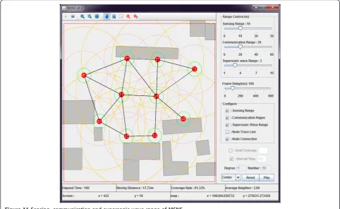
Figure 11Sensing, communication and supersonic wave range of MSNS.

that represents the average number of neighboring sen-sors out of the total sensen-sors.

Viewer provides the information, which is set up in the map toolbar, side configuration panel and base con-figuration panel, and the information on sensors that move to monitor the area depending on visualization.

Figure 11 shows that map objects are expressed by using the GML and processed basically as obstacles. Since GML document keeps the information on large area, it is neces-sary to select the target area to deploy sensors. When the degreeKof sensor is 1 and the number of sensors is 10, the figure shows deployment of sensors, sensing range and number of neighboring sensors that are maintained on average (pink circle: sensing range, orange circle: commu-nication range, green circle: supersonic wave range). And the figure shows the sensing range of the target area in percentage (61.32%) along with the average (2.60) for each neighboring sensor out of all sensors.

6. Performance evaluation

For performance evaluation of the MSNS, it was assumed that sensors moved moderately if the evalua-tion was not based on time and if the average value of virtual force of mobile sensors deployed properly in the target area was smaller than the critical value. Then, the average value was used.

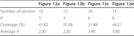
Figure 12 shows the connectivity degree of sensors in the same target area as the one where obstacles are set by the GML and the results of implementing MSNS after changing the number of sensors. Figure 12c, d shows the result that the sensing coverage of the target area diminished when simulation was conducted as the connectivity degree was increased while the number of sensors was kept constant in the same environment as the one in Figure 12a,b. In the different perspective, Fig-ure 12b,d shows the result that the sensing coverage of the target area increased when simulation was con-ducted as the number of sensors was increased while the connectivity degree was kept constant in the same environment as the one in Figure 12a,c. The results of such simulation are shown in Table 2.

Figure 13a,b is the graphs that represent coverage, depending on number of sensors and elapsed unit time, and change in average number of neighboring sensors in the cases where obstacles did not exist and did exist. When the number of sensors was 15, 20, and 25, the

Table 2 Simulation of sensor deployment with connectivity degree

Figure 12a Figure 12b Figure 12c Figure 12d

Number of sensors 10 15 10 15

K 3 3 6 6

Coverage (%) 41.82 55.38 31.88 44.21

AverageK 2.00 2.20 3.40 3.80

Figure 13Number of sensors, coverage with time and average number of neighbor sensor (Rs= 10,Rc= 20,Rw= 3, corner, degreeK

results of simulation were measured. As the time of simulation passed, the coverage increased gradually while the average number of neighboring sensors decreased.

Figure 13b shows that the MSNS coverage algorithm operates in the similar way to that of the existing con-strained coverage, avoiding obstacles.

Figure 14a,b is the graphs that represent coverage, according to degreeK that should be maintained, and change in average number of neighboring sensors in the cases where obstacles did not exist and did exist. As the degreeKincreases, the coverage ratio of the target area decreases while the average number of neighboring sen-sors increases.

Figure 15a,b is the graphs that represent coverage, according toRcand degree K, and change in number of

neighboring sensors in the cases where obstacles did not exist and did exist. In case of Rc > 2Rs, the coverage

ratio was higher while the average number of neighbor-ing sensors due to the given degree Kincreased simi-larly. This result demonstrated that the size of Rc did

not have the significant influence on the increase in average number of neighboring sensors.

7. Conclusion and future research

The MSNS developed in this article is the simulator that provides the information on sensing coverage of the tar-get area where a number of mobile sensors are

randomly deployed. Prior to the MSNS execution, the different connectivity degree is provided for different applications in consideration of the GML-based obsta-cles, which helps infer the number of sensors that are required in the target area and determine coverage ratio of the target area. In most of the previous studies, the connectivity is fixed or limited, or sensing range or communication range of sensor is determined in advance. In addition, other problems are that the infor-mation on location of sensors is displayed by using the screen coordinate, or shape of obstacles is determined in advance. MSNS uses the GML-based GPS coordinate information to utilize terrain coordinate. And based on such information, obstacles are set up so that it is possi-ble to consider obstacles in various shapes. Furthermore, since the actual map coordinate is used, it is possible to estimate the actual coordinate of a sensor that moves on the actual map coordinate. It is also possible to con-duct simulation of various environments since user interface is used to provide connectivity degree of sen-sors, sensing range, supersonic wave range, and number of sensors. The major contribution of this article is the proposal of a new virtual force to guide mobile sensors onto a more optimal path in terms of coverage expan-sion with respect to GPS and obstacle in theory aspect. This is achieved by incorporating the attractive force generated from the centroid of a sensor’s local Voronoi

Figure 14Number of sensors, coverage with degreeKand variation of neighbor sensor (Rs= 10,Rc= 20,Rw= 3, corner, elapsed time

polygon with the repulsive forces generated by obstacles and neighboring nodes.

The future researches include applying probability model, instead of binary model, to sensing range and utilizing MSNS coverage algorithm for self-deployable mobile sensors with such different sensing range model. Another is to consider a more realistic possibility in dis-tortion of sensing/communication range due to obstacles.

Acknowledgements

This research was supported by the IT R&D Program of MKE/KEIT [10035708, “The Development of CPS (Cyber-Physical Systems) Core Technologies for High Confidential Autonomic Control Software"] and also supported by Basic Science Research Program through the National Research Foundation of Korea (NRF) funded by the Ministry of Education, Science and Technology (2011-0025975).

Author details

1

Department of Computer Engineering, Wonkwang University, 344-2 Shinyong-Dong, Iksan 570-749, South Korea2_{Advanced Technology Research}

Center, Korea University of Technology and Education, CheonAn, South Korea3_{Department of Computer Science and Engineering, Seoul National}

University of Science and Technology, Seoul, South Korea4_Embedded

Software Research Department, Electronics and Telecommunications Research Institute, Daejeon, South Korea

Competing interests

The authors declare that they have no competing interests.

Received: 11 June 2011 Accepted: 8 March 2012 Published: 8 March 2012

References

1. R Arkin, K Ali, Integration of reactive and telerobotic control in multi-agent robotic systems, inThird International Conference on Simulation of Adaptive Behavior, (SAB94) [From Animals to Animates], Brighton, England, pp. 473–478 (August 1994)

2. G Tan, SA Jarvis, A-M Kermarrec, Connectivity-guaranteed and obstacle-adaptive deployment schemes for mobile sensor networks. inProc of IEEE ICDCS 2008429_–437 (June 2008)

3. F Xue, PR Kumar, The number of neighbors needed for connectivity of wireless networks. Wirel Netw.10(2), 169–181 (2004)

4. H-J Lee, Y-H Kim, Y-H Han, CY Park, Centroid-based movement assisted sensor deployment schemes in wireless sensor networks, in2009 IEEE 70th Vehicular Technology Conference(September 2009)

5. C-W Lee, S-W Kim, H-J Lee, Y-H Han, D-S Park, Y-S Jeong, Visualization of the constrained coverage of mobile sensor networks based on GML, in4th International Symposium on Cloud and Convergence Computing, Vancouver, Canada, pp. 603_–608 (August 2009)

6. MA Goodrich, Potential fields tutorial. http://www.ee.byu.edu/ugrad/ srprojects/robotsoccer/papers/goodrich_potential_fields.pdf

7. A Howard, MJ Mataric, GS Sukhatme, Mobile sensor network deployment using potential fields: a distributed, scalable solution to the area coverage problem, in6th International Symposium on Distributed Autonomous Robotics Systems (DARS02)(June 2002)

8. S Poduri, GS Sukhatme, Constrained coverage for mobile sensor networks, inIEEE International Conference on Robotics and Automation, New Orleans, LA, pp. 165_–172 (2004)

9. J Chen, MB Salim, M Matsumoto, A single mobile target tracking in Voronoi-based clustered wireless sensor network. J Inf Process Syst.6(4), 17–28 (2010)

10. G Wang, G Cao, TL Porta, Movement-assisted sensor deployment. IEEE INFOCOM 2004.4, 2469–2479 (March 2004)

11. OpenGIS Consortium, Inc, Geography Markup Language [GML], 07-036_Geography_Markup_Language_GML_V3.2.1.pdf.

12. OpenGIS Location Service Core Serviceshttp://www.opengeospatial.org/ 13. Z Guo, S Zhou, Z Xu, A Zhou, G2ST: a novel method to transform GML to

SVG, inProceedings of the 11th ACM international symposium on Advances in

Figure 15Number of sensors, coverage with degreeKand variation of neighbor sensor (Rs= 10,Rc= 20,Rw= 3, corner, sensors =

geographic information systems, OpenGIS Consortium, Inc, pp. 161–168 (November 2003) http://www.opengeospatial.org/docs/02-023r4.pdf. Geography Markup Language (GML) Implementation Specification 14. S Shekhar, RR Vatsavai, N Sahay, TE Burk, S Lime, WMS and GML based

interoperable web mapping system, inGIS: Geographic Information Systems, pp. 106_–111 (2001)

15. M Cardei, MT Thai, Y Li, W Wu, Energy-efficient target coverage in wireless sensor networks, inProc IEEE INFOCOM_’.3, 1976_–1984 (2005)

16. KK Chintalapudi, A Dhariwal, R Govindan, GS Sukhatme, Ad-hoc localization using ranging and sectoring, inIEEE Info-communications(March 2004)

doi:10.1186/1687-1499-2012-95

Cite this article as:Jeonget al.:MSNS: mobile sensor network simulator for area coverage and obstacle avoidance based on GML.EURASIP Journal on Wireless Communications and Networking20122012:95.

Submit your manuscript to a

journal and benefi t from:

7Convenient online submission 7Rigorous peer review

7Immediate publication on acceptance 7Open access: articles freely available online 7High visibility within the fi eld

7Retaining the copyright to your article