Scholarship@Western
Scholarship@Western
Electronic Thesis and Dissertation Repository
12-1-2011 12:00 AM
A System Dynamics Based Integrated Assessment Modelling of
A System Dynamics Based Integrated Assessment Modelling of
Global-Regional Climate Change: A Model for Analyzing the
Global-Regional Climate Change: A Model for Analyzing the
Behaviour of the Social-Energy-Economy-Climate System
Behaviour of the Social-Energy-Economy-Climate System
Mohammad Khaled AkhtarThe University of Western Ontario Supervisor
Slobodan P. Simonovic
The University of Western Ontario
Graduate Program in Civil and Environmental Engineering
A thesis submitted in partial fulfillment of the requirements for the degree in Doctor of Philosophy
© Mohammad Khaled Akhtar 2011
Follow this and additional works at: https://ir.lib.uwo.ca/etd Part of the Civil and Environmental Engineering Commons
Recommended Citation Recommended Citation
Akhtar, Mohammad Khaled, "A System Dynamics Based Integrated Assessment Modelling of Global-Regional Climate Change: A Model for Analyzing the Behaviour of the Social-Energy-Economy-Climate System" (2011). Electronic Thesis and Dissertation Repository. 331.
https://ir.lib.uwo.ca/etd/331
This Dissertation/Thesis is brought to you for free and open access by Scholarship@Western. It has been accepted for inclusion in Electronic Thesis and Dissertation Repository by an authorized administrator of
A SYSTEM DYNAMICS BASED INTEGRATED ASSESSMENT MODELLING OF GLOBAL-REGIONAL CLIMATE CHANGE: A MODEL FOR ANALYZING THE
BEHAVIOUR OF THE SOCIAL-ENERGY-ECONOMY-CLIMATE SYSTEM
(Spine title: System Dynamics Based Integrated Assessment Modelling)
(Thesis Format: Monograph)
by
Mohammad Khaled Akhtar
Graduate Program in Engineering Sciences Department of Civil and Environmental Engineering
A thesis submitted in partial fulfillment of the requirements for the degree of
Doctor of Philosophy
The School of Graduate and Postdoctoral Studies The University of Western Ontario
London, Ontario, Canada
ii
THE UNIVERSITY OF WESTERN ONTARIO School of Graduate and Postdoctoral Studies
CERTIFICATE OF EXAMINATION
Supervisor
______________________________ Dr. Slobodan P. Simonovic
Examiners
______________________________ Dr. Craig Miller
______________________________ Dr. Clare Robinson
______________________________ Dr. Gordon McBean
______________________________ Dr. Evan Davies
The thesis by
Mohammad Khaled Akhtar
entitled:
A System Dynamics based Integrated Assessment Modelling of
Global-Regional Climate Change: A Model for Analyzing the
Behaviour of the Social-Energy-Economy-Climate System
is accepted in partial fulfillment of the requirements for the degree of
Doctor of Philosophy
______________________ _______________________________
iii
ABSTRACT
The feedback based integrated assessment model ANEMI (version 2) represents the society-biosphere-climate-economy-energy system of the earth and biosphere. The development of the ANEMI model version 2 is based on the system dynamics simulation approach that (a) allows for the understanding and modelling of complex global change and (b) assists in the investigation of possible policy options for mitigating, and/or adapting to changing global conditions within an integrated assessment modelling framework. This thesis presents the ANEMI model version 2 and its nine individual sectors: climate, carbon cycle, land-use, population, food production, hydrologic cycle, water demand, water quality, and energy-economy. Two levels of the model are developed and presented here. The first one represents the society-biosphere-climate-economy-energy system on a global scale (ANEMI version 2). The second one is developed for a regional presentation of Canada (ANEMI_CDN). The development of the Canada model is based on the top-down approach and various disaggregation techniques. The disaggregation technique also extends the capability of the ANEMI model version 2 in generating monthly data, while the model runs with yearly time step. To evaluate market and nonmarket costs and benefits of climate change, the ANEMI model integrates an economic approach, with a focus on the international energy stock and fuel price, with climate interrelations and temperature change. The model takes into account all major greenhouse gases (GHG) influencing global temperature and sea-level variation.
iv
of three policy scenarios in both global and Canadian perspectives.
v
DEDICATION
vi
ACKNOWLEDGEMENTS
First of all, I would like to gratefully acknowledge my supervisor Professor Slobodan P. Simonovic for his guidance and indispensable support in completing this research. I greatly admire him for his accessibility and patience, his professionalism and scientific insight. I feel honoured to have him as my supervisor. Thanks are also due to Professor Gordon McBean of the Geography department and Professor Evan Davies of the University of Alberta for their invaluable suggestions at different stages of my study period.
My special thanks go to our project partners from the Economics department at Western: Ph.D. candidate Jacob Wibe, Professor Jim Davies and Professor Jim MacGee. We worked together on the development of the energy-economy sector of the ANEMI model version 2 and without their support the research would not have reached this level.
I am grateful for the support of NSERC (Natural Sciences and Engineering Research Council of Canada) through its Strategic Research Grant to Professor Slobodan P. Simonovic and his collaborators, which funded development of the ANEMI model. I am gratified by my friends in the FIDS office and in Civil and Environmental Engineering at Western, who provided inspiration from time to time, and much-needed escapes from work: Shubhankar, Vasan, Hyung, Pat, Shohan, Tarana, Dragan, Ponselvi, Angela, Lisa, Vladimir, Jordan, Dejan, Samiran, Amin, and Abhishek. Thanks to my friends in London: Iftekhar, Shahed, Bahalul, Zahid and Anis for helping me time to time which made my life easier.
vii
beloved wife and son. Their sacrifice, presence and smile have revived me every day for tomorrow's struggles; they are the very reason why I am here and am striving.
viii
TABLE OF CONTENTS
CERTIFICATE OF EXAMINATION ... ii
ABSTRACT ... iii
DEDICATION... v
ACKNOWLEDGEMENTS ... vi
TABLE OF CONTENTS ... viii
LIST OF TABLES ... xiii
LIST OF FIGURES ... xv
CHAPTER 1 ... 1
1 INTRODUCTION ... 1
1.1 Climate Change ... 1
1.1.1 Global Climate Change ... 2
1.1.2 Climate Change Research ... 4
1.2 Global Climate Modelling ... 8
1.3 Regional Climate Modelling ... 8
1.3.1 Benefits of Regional Climate Modelling ... 9
1.3.2 Limitations of Regional Climate Modelling ... 10
1.4 Climate Research in Support of Policy Development ... 10
1.5 Research Objectives ... 13
1.6 Contributions of the Research ... 15
1.7 Thesis Organization ... 16
CHAPTER 2 ... 19
2 LITERATURE REVIEW... 19
2.1 Climate Change Modelling ... 19
ix
2.2.2 Basics of System Dynamics Modelling ... 26
2.2.3 Application of System Dynamics Modelling to Climate Policy Assessment ... 28
2.2.4 Application of System Dynamics Modelling to Water Resources Management ... 29
2.2.5 System Dynamics Modelling in Engineering ... 32
2.3 Optimization ... 35
2.3.1 Applications of Optimization ... 35
2.3.2 Most Used Optimization Energy-Economy Models ... 37
2.4 Integrated Assessment Modelling (IAM) ... 39
2.4.1 The Emergence of IAMs as a Science-Policy Interface ... 39
2.4.2 Classification of IAMs ... 39
2.4.3 Application of Integrated Assessment Models ... 40
2.4.4 Challenges for IAM Studies... 49
CHAPTER 3 ... 51
3 GLOBAL MODEL OF THE SOCIAL-ENERGY-ECONOMY-CLIMATE SYSTEM ... 51
3.1 Description of Individual Model Sectors ... 52
3.1.1 The Climate Sector ... 54
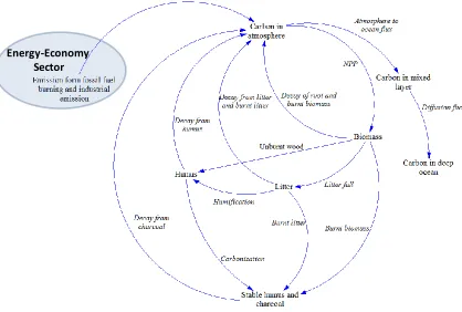
3.1.2 The Carbon Sector ... 66
3.1.3 The Energy-Economy Sector ... 75
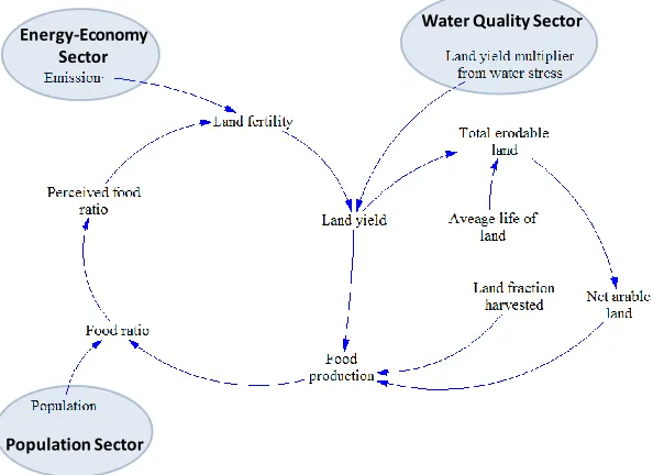
3.1.4 The Food Production Sector ... 91
3.1.5 The Land-Use Sector ... 98
3.1.6 The Population Sector ... 103
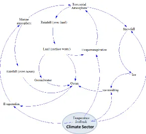
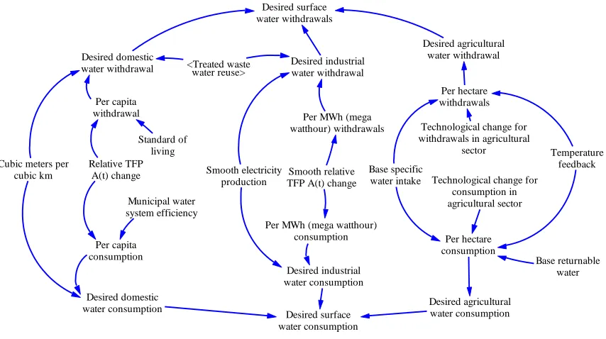
3.1.7 The Water Resources Sectors ... 108
x
3.2.1 Feedbacks within the ANEMI Model Version 2 Water Sectors ... 136
3.2.2 Feedbacks in the ANEMI Model Version 2 Non-Water Sectors ... 140
3.2.3 Summary ... 144
CHAPTER 4 ... 146
4 GLOBAL MODEL EXPERIMENTATION... 146
4.1 ANEMI Model (version 2) Performance ... 146
4.1.1 Water Use... 148
4.1.2 Sea-Level Rise ... 150
4.1.3 Global Population ... 151
4.1.4 Energy based CO2 Emissions and Energy Production ... 153
4.1.5 Gross Domestic Product (GDP) ... 157
4.1.6 Physical Characteristics of the Earth System... 158
4.1.7 Summary ... 167
4.2 ANEMI Model Version 2 Simulations ... 168
4.2.1 Carbon Tax Scenario... 169
4.2.2 Increase Water Use Scenario ... 170
4.2.3 Food Production Increase Scenario ... 171
4.3 Global ANEMI Model (Version 2) Analyses Results ... 172
4.3.1 Global Carbon Tax Scenario ... 172
4.3.2 Global Water Use Scenario ... 179
4.3.3 Global Food Production Scenario ... 185
CHAPTER 5 ... 192
5 REGIONAL MODEL OF THE SOCIAL-ENERGY-ECONOMY-CLIMATE SYSTEM ... 192
xi
5.1.2 The Land-Use Sector ... 195
5.1.3 The Water Sectors ... 196
5.1.4 The Food Production Sector ... 199
5.1.5 The Energy-Economy Sector ... 200
5.2 Disaggregation Procedure ... 203
5.2.1 Temporal Disaggregation... 203
5.2.2 Spatial Disaggregation ... 205
5.2.3 Disaggregation Data Description ... 206
CHAPTER 6 ... 209
6 REGIONAL MODEL EXPERIMENTATION ... 209
6.1 Regional ANEMI Model (ANEMI_CDN) Performance ... 209
6.1.1 Water Use... 209
6.1.2 Population ... 212
6.1.3 Land-Use ... 213
6.1.4 Energy-Economy ... 214
6.2 Regional ANEMI Model (ANEMI_CDN) Analyses ... 215
6.2.1 Canada Carbon Tax Scenario ... 216
6.2.2 Canada Water Use Scenario ... 219
6.2.3 Canada Food Production Increase Scenario ... 223
6.3 Summary ... 228
CHAPTER 7 ... 230
7 OPTIMIZATION AND SIMULATION FOR THE INTEGRATED ASSESSMENT MODELLING ... 230
7.1 Optimization Simulation Model ... 231
xii
7.1.3 Mathematical Formulation of the Optimization-Simulation Problem in
ANEMI Version 2 ... 237
7.2 Limitations ... 248
CHAPTER 8 ... 250
8 DISAGGREGATION FOR REGIONALIZATION OF ANEMI MODEL ... 250
8.1 Disaggregation Modelling ... 252
8.1.1 Temporal Disaggregation... 253
8.1.2 Spatial Disaggregation ... 262
8.2 Performance Evaluation ... 263
CHAPTER 9 ... 266
9 CONCLUSIONS ... 266
9.1 Representation of the Past ... 267
9.2 How the Future May Look Under Various Policy Choices ... 269
9.2.1 Carbon Tax Implementation ... 270
9.2.2 Increased Water Consumption ... 270
9.2.3 Increased Food Production ... 271
9.3 Optimization Simulation of ANEMI Model ... 272
9.4 Regionalization ... 273
9.5 Adjudication ... 274
9.6 Recommendations for Future Research ... 275
REFERENCES ... 278
APPENDIX A: Important Definitions from Economics ... 303
APPENDIX B: Atmosphere-Ocean Global Climate Models ... 306
APPENDIX C: Data Processing of GCM‘s ... 315
xiii
LIST OF TABLES
Table 2.1: List of Integrated Assessment Models (most used) ... 43
Table 3.1: Initial temperatures and configuration of ocean layers (°C and m, respectively) . 66 Table 3.2: Parameters of the flow through the terrestrial biosphere ... 72
Table 3.3: Initial carbon stock and base surface density of NPP, σ(NPPj)0, values ... 72
Table 3.4: Initial fossil fuel reserve (in trillion GJ) ... 90
Table 3.5: Transfer matrix of area between ecosystems (Mha yr-1) in 1980 ... 100
Table 3.6: Major stocks of water, and values used in the ANEMI model version 2 (in km3) ... 110
Table 3.7: Hydrologic flows and initial flow values used in the ANEMI model version 2 (in km3 yr-1) ... 111
Table 3.8: Treated wastewater reuse allocations to water use sectors (after Davies, 2007) . 122 Table 3.9: Summary of the ANEMI model modifications ... 145
Table 4.1: Assessed global water withdrawals and consumption (in km3/yr) ... 149
Table 4.2: Projected global water withdrawals and consumption (in km3/yr) ... 149
Table 4.3: Comparison of historical global population (in billions) ... 152
Table 4.4: Comparison of future global population (in billions) ... 152
Table 4.5: Comparison of historical industrial emissions (in Gt C/yr) ... 155
Table 4.6: Simulated industrial emissions (in Gt C/yr) ... 157
Table 4.7: Global surface temperature change (in oC) ... 160
xiv 2
Table 4.10: Future global atmospheric CO2 concentration (ppm) ... 164
Table 4.11: Historical net primary productivity (NPP), 1980-2005 ... 166
Table 4.12: Future net primary productivity (NPP) ... 167
Table 5.1: Population by age-group of 1980 (DESA, 2011) ... 195
Table 5.2: Initial land transfer matrix for Canada (Mha yr-1, in 1980) ... 196
Table 5.3: Initial value for irrigated area and electricity production (1980) ... 198
Table 5.4: Assumed future fossil fuel discovery (Canada) in billion GJ ... 202
Table 5.5: GCM models used for the regionalization of the temperature and rainfall data . 208 Table 8.1: Monthly average temperature (Kelvin) of Canada ... 264
xv
LIST OF FIGURES
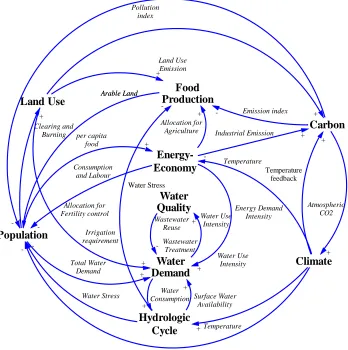
Figure 3.1: ANEMI model version 2 structure ... 54
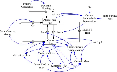
Figure 3.2: Model structure of the comprehensive climate sector ... 56
Figure 3.3: Model structure of the simplified climate sector (after Nordhaus, 1994) ... 57
Figure 3.4: Causal loop diagram of the comprehensive climate sector ... 58
Figure 3.5: Causal loop diagram of the simplified climate sector ... 59
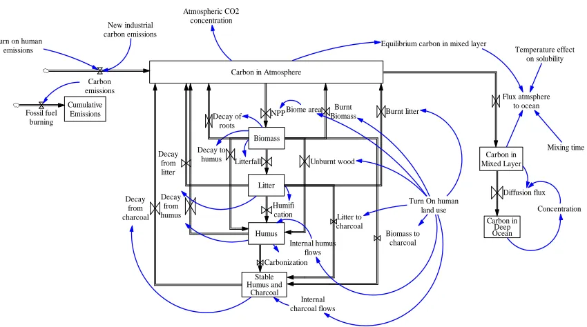
Figure 3.6: Model structure of the ANEMI model version 2 carbon sector ... 67
Figure 3.7: CO2 solubility of ocean water (after Larryn et al., 2003) ... 68
Figure 3.8: Causal loop diagram of the ANEMI version 2 carbon sector ... 69
Figure 3.9: Causal loop diagram of ANEMI energy-economy sector ... 77
Figure 3.10: Yearly food production (billion veg-eq-kg) ... 93
Figure 3.11: Model structure of the ANEMI version 2 food production sector ... 94
Figure 3.12: Causal loop diagram of the ANEMI version 2 food production sector... 96
Figure 3.13 Model structure of the ANEMI version 2 land-use sector ... 99
Figure 3.14: Causal loop diagram of the ANEMI version 2 land-use sector ... 101
Figure 3.15: Model structure of the ANEMI version 2 population sector ... 104
Figure 3.16: Causal loop structure of the ANEMI version 2 population sector ... 105
Figure 3.17: Model structure of the ANEMI version 2 hydrologic cycle sector ... 110
Figure 3.18: Causal loop diagram of the ANEMI hydrologic cycle sector ... 112
xvi
Figure 3.21: Model structure of the ANEMI version 2 water quality sector ... 121
Figure 3.22: Causal loop diagram of the ANEMI model version 2 water quality sector ... 123
Figure 3.23: ANEMI model version 2 structure ... 135
Figure 3.24: Feedback loops within ANEMI model version 2 water sectors ... 137
Figure 4.1: Comparison of global population projection ... 153
Figure 4.2: Comparison of heat energy production ... 154
Figure 4.3: Comparison of electric energy production ... 154
Figure 4.4: Comparison of industrial carbon emissions ... 156
Figure 4.5: Comparison of GDP per capita ... 158
Figure 4.6: Comparison of atmospheric CO2 concentration ... 165
Figure 4.7: Energy used to produce electricity ... 172
Figure 4.8: Energy used to produce heat energy... 173
Figure 4.9: Global energy consumption... 174
Figure 4.10: Global CO2 emissions from fossil fuel ... 174
Figure 4.11: Global atmospheric CO2 concentration ... 175
Figure 4.12: Global atmospheric temperature change ... 176
Figure 4.13: Global sea-level rise ... 176
Figure 4.14: Global population ... 177
xvii
Figure 4.17: Global GDP change ... 179
Figure 4.18: Global available surface water ... 180
Figure 4.19: Global water-stress ... 181
Figure 4.20: Global food production ... 181
Figure 4.21: Global population ... 182
Figure 4.22: Global CO2 emissions from fossil fuel ... 183
Figure 4.23: Global atmospheric CO2 concentration ... 183
Figure 4.24: Global GDP ... 184
Figure 4.25: Global atmospheric temperature ... 184
Figure 4.26: Global sea-level rise ... 185
Figure 4.27: Global food production ... 186
Figure 4.28: Global available surface water ... 187
Figure 4.29: Global water-stress ... 187
Figure 4.30: Global population ... 188
Figure 4.31: Global CO2 emissions from fossil fuel ... 189
Figure 4.32: Global GDP ... 189
Figure 4.33: Global atmospheric CO2 concentration ... 190
Figure 4.34: Global atmospheric temperature ... 191
xviii
Figure 6.1: Domestic water withdrawals (Canada) validation... 210
Figure 6.2: Industrial water withdrawals (Canada) validation... 211
Figure 6.3: Agricultural water withdrawals (Canada) validation ... 211
Figure 6.4: Population of Canada (validation results) ... 212
Figure 6.5: Forest area (Canada) validation ... 213
Figure 6.6: Cultivated area (Canada) validation ... 214
Figure 6.7: Real GDP per capita for Canada ... 215
Figure 6.8: GDP per capita (Canada) ... 217
Figure 6.9: Total energy used in the production of aggregate energy services (Canada) ... 218
Figure 6.10: Industrial emissions from fossil fuel (Canada)... 219
Figure 6.11: Available surface water (Canada) ... 220
Figure 6.12: Water-stress (Canada) ... 220
Figure 6.13: Food production (Canada) ... 221
Figure 6.14: Population (Canada) ... 222
Figure 6.15: CO2 emissions from fossil fuel (Canada) ... 222
Figure 6.16: GDP (Canada) ... 223
Figure 6.17: Food production (Canada) ... 224
Figure 6.18: Available surface water (Canada) ... 225
xix
Figure 6.21: CO2 emissions from fossil fuel (Canada) ... 227
Figure 6.22: GDP (Canada) ... 227 Figure 7.1: Basic computational flow chart of the energy-economy sector of the ANEMI model (ANEMI version 2 and ANEMI_CDN) ... 237 Figure 7.2: Schematic view of simulation based optimization scheme ... 238 Figure 8.1: Monthly temperature comparison between analyzed and simulated data ... 265
CHAPTER 1
1
INTRODUCTION
This thesis presents the ANEMI version 2 and the ANEMI_CDN: nine-sector global and regional versions of an integrated assessment model that combines a system dynamics-based simulation with a non-linear optimization procedure. (―ANEMI‖ is an ancient Greek term for the four winds, heralds of the four seasons; here ANENI links physical system such as the climate and hydrological- and carbon cycles with the socio-economic systems that change them: the economy, land-use, population change, and water use and quality). In representing the social-energy-economy-climate system, the two versions of this model function to clarify the fundamental feedbacks among the system‘s interrelated sectors. Hence the model helps to increase our knowledge of climate change and its range of impacts, and to assist in the adaption of suitable policy strategies. The disaggregation modelling approach that we have adopted allows the global model of the ANEMI version 2 to be converted into a regional version for Canada. The ANEMI_CDN can thus support the attempts to achieve environmental and economic benefits for all Canadians.
1.1 Climate Change
The term climate usually brings to mind an average regime of weather. Here we are not so much interested in particular climates as we are in the Earth‘s climatic system as a whole. The climatic system consists of those properties and processes that are responsible for any given climate and its variations. According to Berkofsky et al. (1981), the properties of the climatic system can be broadly classified as thermal, which include the temperature of the air, water, ice, and land; kinetic, which include the wind and ocean currents, together with the associated vertical motions, and the motion of ice masses;
aqueous, which include the air‘s moisture or humidity, the cloudiness and cloud water
which include the pressure and density of the atmosphere and ocean, the composition of the (dry) air, the oceanic salinity, and the geometric boundaries and physical constants of the system. The complete climatic system therefore consists mainly of five physical components: the atmosphere, hydrosphere, cryosphere, lithosphere, and biosphere.
The earth‘s climates have always been changing, and the magnitude of these changes has varied from place to place and from time to time. In some places, the yearly changes are so small as to be of minor interest, while in others the changes can be catastrophic. The increasing evidence from paleoclimatic specimens shows that the earth‘s climates have undergone long series of complex natural changes in the past. The further realization that human activities could expedite the process has aroused great interest in the problems related to climate change and variation.
The last twenty years has witnessed a growing scientific consensus that global warming is underway. Within the scientific community, it is largely accepted that climate change will have significant- and mostly negative- consequences for humankind.
1.1.1
Global Climate Change
Climate change has been a subject of intellectual interest for many years. What compels our interest is the growing awareness of the relationship between climate change and our social and economical stability. As the climate is always changing, scientific research focuses on such questions as how large these future changes will be, and where and how rapidly they will occur.
structures of human civilizations are sensitive to atmospheric changes. A major climate change could conceivably destabilize a civilization‘s economic and social structure. Civilizations depend on such factors as food production and water availability and these factors implicitly depend on the climate. Unfortunately, our climate system is in trouble, having warmed by over 0.7 degree Celsius in the last 100 years (Hare, 2009). Most of the warming since at least the mid-twentieth century is very likely due to human activities. Even after 20 years of international attention, emissions (GHGs, particularly CO2) from
fossil fuel burning and land-use change continue to grow rapidly. As a result, the concentration of CO2 has not only increased; it now exceeds any value after continuous
instrumental measurement. This current trend of rising CO2 concentration in turn
increases the atmospheric temperature rapidly through radiative forcing.
Modern climate change appears to be on the point of exceeding the threshold of natural variability. This is largely a result of human-induced changes in atmospheric composition (Karl and Trenberth, 2003). The sources of these atmospheric perturbations include emissions associated with energy use, urbanization and land-use changes. While many uncertainties remain about the rate of climate change, it is indubitable that these changes will be increasingly manifested in important and tangible ways: extremes of temperature and precipitation, decreases of seasonal and perennial snow and ice extent, and sea-level rise.
The climate system evolves in time under the influence of its own internal dynamics and
due to changes in external factors that affect climate (called ‘forcings’). External forcing
include natural phenomena such as volcanic eruptions and solar variations, as well as
human-induced changes in atmospheric composition. Solar radiation powers the climate
system. There are three fundamental ways to change the radiation balance of the Earth:
1) by changing the incoming solar radiation (e.g., by changes in Earth’s orbit or in the
altering the longwave radiation from Earth back towards space (e.g., by changing
greenhouse gas concentrations). Climate, in turn, responds directly to such changes, as
well as indirectly, through a variety of feedback mechanisms (Le Treut et al., 2007).
There is no doubt that the earth‘s climates have changed in the past and will change in the future. Along with an extended database, climate change theory and dynamical models of climate change must focus more on the determination of the climate‘s predictability.
1.1.2
Climate Change Research
For more than a decade, climate change has been the focus of much research and analysis. Although we have considerable knowledge of the broad characteristics of the climate, we are still having difficulties in understanding the major processes of climate change. This compels climate change researchers not only to study each individual component of the climatic system but also the world‘s oceans, the ice masses, the exposed land surface and importantly, the socio-economic system. Only through such studies can an integrated modelling approach make significant advances in understanding the indefinable and complex process of climatic change. Despite the global implications of the problem, the overwhelming majority of the researchers involved worldwide in studying the problem and its possible solutions are from industrialized countries. Participation of lesser-industrialized countries has been limited.
(ALPEX) in 1982. These field experiments contributed to major improvements in Numerical Weather Prediction. GARP operates under the auspices of the World Meteorological Organization and the International Geodetic and Geophysical Union.
In order to improve our understanding of the complex interactions between the climate system, ecosystems and human activities, the research community develops and uses scenarios. These scenarios are intended to plausibly portray the future state of socioeconomic, technological and environmental conditions, the emissions of greenhouse gases and aerosols, and the climate. The model-based scenarios used in climate change research are developed using a sequential process focused on a step-by-step and time-consuming delivery of information between separated scientific disciplines (Moss et al., 2010). Currently, climate change researchers from different disciplines deal primarily with four scenarios of future radiative forcing, where radiative forcing refers to the change in the balance between incoming and outgoing radiation to the atmosphere caused by changes in atmospheric constituents, such as carbon dioxide.
It is the intersectoral aspects of climate change, at once socio-economic and environmental, that makes it such a complex problem. Thus the economics of climate change are even less well-understood than climate science, and in the latter uncertainties remain in transport modelling of the greenhouse gas (GHG) pollutants through the atmosphere and the effect of GHGs on the atmospheric components (atmospheric temperature, ocean temperature, rainfall, and etc.). Nowadays, many aspects of climate change are under studied in isolation. But at the same time many researchers are currently combining the socio-economic part of climate change with the scientific aspect of climate change for policy option analysis under projected climatic (climate change) conditions. Such models are known as integrated assessment models (IAMs). Kelly & Kolstad (1999) broadly define an integrated assessment model as any model that combines scientific and socio-economic aspects of climate change primarily for the purpose of assessing policy options for climate change control. Some examples are: Dowlatabadi and Morgan (1995; 1993a), Kolstad (1996), Lempert et al. (1996), Manne, Mendelsohn, and Richels (1995), Nordhaus (1994), and Peck and Teisberg (1992).
According to Weyant et al. (1996), an integrated assessment model is one that draws on knowledge from research in multiple disciplines. Weyant et al. (1996) mentioned three purposes of such models: (1) to assess climate change control policies (for example, the computation of the optimal climate control policy), (2) to constructively force multiple dimensions of the climate change problem into the same framework (for example, in identifying the driving forces behind climate change by identifying to which sectors climate change is most sensitive), and (3) to quantify the relative importance of climate change in the context of other environmental and non-environmental problems facing humankind (for example, in ranking the benefits of climate change control with improving sanitation or improving medicine in developing countries).
The other type of IAM is an optimization model. The IAM serves two purposes: (a) to find the optimal policy which trades off expected costs and benefits of climate change control or the policy which minimizes costs of achieving a particular goal, and (b) to simulate the effect of an efficient level of carbon abatement on the world economy (Kelly & Kolstad, 1999). Usually, policy evaluation models deal with a single exogenous specified policy and estimate the effect of that policy on individual sectors, as well as the combined effect on the projected future. In contrast, policy optimization models search for optimal policy. While this is a complex process, these models produce simpler representations at the sectoral level. So, the advantage of a policy evaluation model over an optimization model is in its detailed description of the physical, economic and social aspects of the very complex climate change problem. Therefore, these types of IA models very much depend on the skill of the modeler in taking into account how consumers and producers behave. Such models could face problems when dealing with scarce resources or environmental constraints. On the other hand, an optimization model deals with complex policies that are dependent on state variables and economic growth. The optimization model therefore allows producers and consumers to determine endogenously the optimal mix of GHG intensive and non-GHG intensive fuels given a climate change control policy, while in the policy evaluation model requires the modeler to specify exogenously the mix of fuel used.
1.2
Global Climate Modelling
Global climate is a result of the complex interactions between the atmosphere,
cryosphere (ice), hydrosphere (oceans), lithosphere (land), and biosphere (life), fueled by
the non-uniform spatial distribution of incoming solar radiation (Stute et al., 2001).
A general circulation model is developed on the basis of fluid dynamics and thermodynamics and it describes the atmosphere and ocean in an explicit way. GCMs (see Appendix B) provides a great opportunity to study the past, present and future climatic system, including global ocean circulation (Stute et al., 2001).
Understanding historical events and processes (paleoclimatic period) is essential to understand the interrelationship among different components of the biospheric system and their feedbacks. This acquired knowledge forms the basis of the model development, on which future climate forecasting is carried out.
The global modelling deals with the whole globe rather than only a part of the sphere and acts like a big brother or a big picture thinker to the regional model, by providing it with boundary conditions.
1.3
Regional Climate Modelling
detailed processes of regional to local conditions. The relatively high resolution and details construction of RCMs enables the researcher to visualize key input to climate impact studies and to deal with possible damages and opportunities related to climate variability and change. Nowadays, regional climate models are used by a wide range of scientific communities around the world. Both the regional and global models have more or less the same objective of regional and global weather forecasting. Over the past 20 years, the development of regional climate models has led to increased resolution and longer model runs. Applications of regional climate models span both the past and possible future climates, facilitating climate impact studies, information and support to climate policy, and adaptation.
As the climate doesn‘t have any geographic boundary, the climate in any one region is affected by the rest of the globe. Boundary conditions consist of the information produced when the large-scale circulation impinges on regional model domain. Where the large-scale circulation is directed out of the domain, boundary conditions absorb the regional climate models (RCMs) information. (Typically, a regional model does not provide information back to a GCM.) These lateral boundary conditions apply along the sides of the regional domain (Rummukainen, 2010).
1.3.1
Benefits of Regional Climate Modelling
The main potential of regional modelling is fine resolution. Higher resolution improves
the representation of any specific area such as a water body, rainfall, surface temperature,
mountain ranges, lakes, and estuaries, as well as other surface features. These give rise to
local or regional circulation and precipitation features, temperature modifications, winds,
and so on. Such higher resolution is beneficial for synoptic and mesoscale systems
1.3.2
Limitations of Regional Climate Modelling
The quality of a regional climate model is not only dependent on the boundary condition
but also the quality of the model itself. GCMs have the skill, but suffer from systematic
biases (Rummukainen, 2010). A systematic error in GCMs can easily hinder the model
improvement because of non-local processes. RCM evaluation is often done with
so-called perfect boundary condition simulations, where the boundary conditions are derived
from global meteorological analyses or reanalyses that are compilations of observed,
rather than simulated conditions.
Availability of suitable observational data limits model evaluation. Even though regional
climate models are run at relatively high resolution, they still suffer from resolution
(scale) problems, as point data sets are collected at meteorological stations, ocean buoys,
and such. This is a complication particularly for the evaluation of many kinds of
extremes, as climate data generated by RCMs (gridded data) are more homogenous in
space compared to observations (Rummukainen, 2010). Another important limitation is
the relatively high demand of computational resources which can put a limit on the
number, resolution, or length of RCM runs.
1.4 Climate Research in Support of Policy Development
The development of environmental policies is not an easy process. It requires an effective science-policy interface. Without an effective link between the two domains, sound evidence-based policies are difficult to achieve. The importance of science in policy is specifically recognized in the Canadian federal government context. In A Framework for Science and Technology Advice: Principles and Guidelines for the Effective Use of
Science advice has an important role to play by contributing to government decisions
that serve Canada’s strategic interests and concerns in areas such as public health and
safety, food safety, environmental protection, sustainable development, innovation, and
national security. The effective use of science advice may also contribute to Canada’s
ability to influence international solutions to global problems (Government of Canada, 2000).
At a national level, the development of science and policy linkages requires (at a minimum) the perception among policy makers that a particular issue is of importance. In both developing and developed countries, long-term global environmental issues have typically been overshadowed by more pressing national and international issues. The de-emphasis in political dialogue on climate change is therefore very common in many countries and regions. Because of the lack of political interest in the issue, the progress in our knowledge of climate has been due to diligence of the large number of climate researchers.
From a scientific perspective, the development of the ANEMI model version 2 contributes to an increased understanding of climate change. It improves the representations of the physical processes involved in the climate system and the carbon cycle, and includes the socio-economic sectors and activities that govern interactions with the biophysical system, especially those that influence or control anthropogenic emissions. It applies the system dynamics simulation methodology, since it can both deal with long term delays, multiple feedback processes, and other elements of dynamic complexity and also provide for easy integration of scientific concepts of social, natural and engineering sciences.
impact of the variables that a policy can affect. This will help policymakers (a) to determine the beneficial effects of different climate change policies, (b) to improve the ability of society to adapt to the detrimental effects of climate change, and (c) to avoid the worst possible outcomes.
As per Popovich et al. (2010), the innovative aspects of the research on science policy communication include the process by which the research team collected policy-related information and how it interacted with the policy domain. While the technical model development proceeded at the University of Western Ontario, key partners in the Canadian federal government were involved from the departments of Environment, Finance, Natural Resources, Fisheries and Oceans and Agriculture. These partners remained engaged throughout the entire process of both the model (ANEMI version 2, ANEMI_CDN) development and have provided useful guidance and feedback. Science policy dialogue was established through the consultation sessions, workshops and direct interviews (see Popovich et al., 2010).
1.5
Research Objectives
The global climate has been changing due to human activities and is projected to keep changing even more rapidly. The consequences of climate change could be devastating, with increased atmospheric greenhouse gas concentrations resulting in large-scale, high-impact, non-linear, and potentially abrupt and irreversible changes in physical and biological systems (Mitchell, 2009).
Global climate models offer the best approach to understanding the physical climate system. At various resolutions, they capture the basic behaviour of the physical processes that drive the climate. However, these models focus only on natural systems, and do not represent socio-economic systems that affect and are affected by natural systems. The most common approach to combining socio-economic and biophysical systems involves applying projected trends (scenarios) to ‗drive‘ the climate model. But such an approach disregards the existing dynamic feedbacks. This research tries to bridge such gaps by deploying an integrated assessment modelling approach within a system dynamics simulation framework.
population are incorporated in the ANEMI model version 2 and feedbacks between the
energy-economy and the environment are more fully modeled?
The earlier version of the ANEMI model version 1 (developed by Davies (2007; 2009) and later reported by Davies and Simonovic (2008; 2010)) runs at a global scale, where the climate related regional impact assessment and resource management is not an option. Under such condition a regional integrated assessment model ANEMI_CDN is developed from the ANEMI model version 2 with disaggregation approach. Hence the second objective is to provide the Canadian government with a scientifically credible tool useful for policy: a system dynamics based model, connecting science, governance, economy, energy, and the environment. Under this objective a more particular research question is raised: What would the future path of the major variables of the socio-energy-economy-climate system in Canada under different policy options and will they differ much from
the global perspective?
The previous version of the ANEMI model (version 1) was facing challenges in defining better policy-oriented decision making regarding energy consumption. This difficulty was related to the absence of a market clearing mechanism (see Appendix A) in the energy-economy sector. For a dependable ANEMI model version 2, the integration of such a mechanism becomes necessary, and this turns out to be the third objective of this research work.
implemented to explore the suitability, as well as to enhance the regionalization process of the ANEMI_CDN model.
1.6
Contributions of the Research
In general, my research is focused on the development of an integrated assessment model of the social-energy-economy-climate system. In this connection an earlier version of the ANEMI model (version 1.2) structure has been utilized with the incorporation of new important sectors along with required modification of the existing sectors. Moreover, a regional version of ANEMI model (ANEMI_CDN) is developed specifically for Canada in context of local climate change study. More specifically, my research contributions are divided into several areas that include:
a) Nine-sector integrated assessment model (ANEMI version 2) for the
social-energy-economy-climate system
b) Integration of optimization within the system dynamics simulation framework
Apart from the simulation modelling, the optimization model is generally used in analyzing complex decision making processes. The main advantage of an optimization model is its ability to deal with hundreds of possibilities and figure out the optimal decision within a short span of time and resources. The ANEMI version 2 and ANEMI_CDN model introduces the integration of an optimization scheme within a system dynamics simulation structure, where the optimal plan/path is updated at each time step of the simulation interval. Therefore, with the introduction of such unique integration approach (simulation based optimization) in the field of integrated assessment modelling, both the ANEMI version 2 and ANEMI_CDN models are becoming more robust and reliable.
c) Implementation of a suitable disaggregation technique within the system
dynamics simulation framework
The basic goal of disaggregation modelling is to allow the preservation of statistical properties at more than one level. The important properties that are always desirable to preserve at all levels are means, variables, the probability distribution of values, and some covariances. The regionalization approach of the ANEMI_CDN model is basically a top-down approach (also known as step-wise design), where both spatial and temporal disaggregation is possible. Inclusions of such a disaggregation modelling technique offers the ANEMI_CDN model an ambitious future in regionalizing the global model.
1.7
Thesis Organization
this chapter describes the research goal, as well as the contribution of the research under feedback based integrated assessment modelling framework. An argument is made that most climate change modelling is gradually moving towards this newer, more integrative approach, as awareness grows of the need for a more comprehensive approach towards global change research
Chapter 2 brings a narrative description of the different type of modelling, including climate change modelling, system dynamics modelling, integrated assessment modelling and optimization, along with their applications.
Chapter 3 explains all the important sectors of the global ANEMI model version 2. This chapter also focuses on the feedback based interaction between and within different sectors.
Chapter 4 includes ANEMI model version 2 experimentation including: performance investigation, scenario formulation, simulation and analyses of simulated results.
Chapter 5 describes all the regionalized sectors of the regional model ANEMI_CDN along with a brief description of the disaggregation procedure.
Chapter 6 deals with the regional model ANEMI_CDN experimentations through model performance investigation, simulation and analyses of simulated results.
Considering the broad sectoral representation and level of complexity of the model two additional chapters (Chapters 7 and 8) are added to deliver a clear understanding of the research work.
Chapter 7 introduces the optimization procedure within the system dynamics simulation framework. Therefore, with this integration approach many of the advantages of the optimization are now incorporated into the system dynamics based simulation framework of the ANEMI model.
temporal disaggregation is carried out to regionalize the global rainfall and temperature data for the regional model ANEMI_CDN.
Chapter 9 concludes the dissertation. It describes the overall success of the research in addressing the objectives and related questions. The last part provides a set of recommendations for future research.
CHAPTER 2
2
LITERATURE REVIEW
This chapter reviews some of the literature related to climate change modelling, system dynamics modelling, integrated assessment modelling and optimization procedures. Nowadays there are numerous climate change models; they function to predict future changes in climatic conditions and to help formulate mitigation policies. Integrated assessment models are especially useful in these regards, since they can provide insight into the interaction between different sectors of a larger system. The component models of individual sciences (natural or social) cannot do this.
Integrated assessment models for the study of climate change developed within the field of system dynamics modelling. A brief description of this development follows later in this chapter. We will also review some existing optimization models for the energy-economy sector. It is necessary to elucidate the application of optimization procedures while selecting the set of decision variables in maximizing/minimizing the objective function.
2.1
Climate Change Modelling
of physical processes, has acquired a good reputation within the scientific community. GCMs are used to assess strategies for climate change mitigation and adaptation. A large range of other models are used for estimating future warming and its impacts, costs of climate change mitigation and the role of technology, as well as policy analyses: energy models, integrated assessment models, and Earth system models.
The Integrated Assessment Society defines the integrated assessment (IA) ‗as the scientific ‗‗meta-discipline‘‘ that integrates knowledge about a problem domain and makes it available for societal learning and decision making processes‘ (TIAS, 2011). Predicting future global climate change requires an interdisciplinary outlook that takes into account the physical, social, and political sciences. So the sectors required to understand climate science are: oceanography, atmospheric dynamics, vulcanology, solar physics, carbon cycle analysis, radiation calculations, ice sheet modelling, paleoclimatology, and atmospheric chemistry. Such a large number of sectoral representations can help us to derive real policy-relevant insights (Harremoes and Turner, 2001; Hope, 2005; Schneider, 1997; Weyant et al., 1996).
In order to understand anthropogenic climate forcing (human-induced climate change) and its effects on natural and human systems, the researcher must coordinate the knowledge from numerous disciplines or fields of inquiry, including economics, engineering, energy, agriculture, health sciences, epidemiology, ecosystems, water resource management, coastal processes, fisheries, and coral reef ecology (Sarofim and Reilly, 2011). Economists also employ multi-equation computer models in their approach to climate change.
For a single 100-year projection, these models require roughly few months to complete (Sarofim and Reilly, 2011). Integrated assessment model (IAM) developers are therefore concerned with bringing together the different earth system components. Such models should also need to be computationally efficient to solve 100-year integrations within a few minutes.
As IAMs aim to integrate different disciplines, they run the risk of becoming extremely complex (van Vuuren, 2011). The most obvious remedy for such excessive complexity is to simplify the climate system and the carbon cycle, which in many IAMs consists of only a few equations (Goodess et al., 2003). Despite the potential drawbacks, IAMs are used to explore the socioeconomic and technological drivers of greenhouse gas emissions and the policies for constraining these emissions from a long-term, global perspective.
Researchers also include both the biophysical and economic systems in their cost assessments of climate protection. In IAMs this is done first by combining the important components of biophysical and economic systems, and then converting them into a single integrated system. Such an approach is capable of delivering a suitable framework that can combine knowledge from a wide range of disciplines. As per IPCC (2001), ―these models strip down the laws of nature and human behaviour to their essentials to depict
how increased GHGs in the atmosphere affect temperature, and how temperature change
causes quantifiable economic losses‖.
2.2
System Dynamics Simulation Modelling
A system is a combination of components, which act together in achieving a specific objective. A component is a single functioning unit of a system (Ogata, 2004). Systems are not limited to physical ones; the concept of a system can be extended to abstract dynamic phenomena, such as those encountered in economics, transportation, population growth, biology, and climate science.
A system is considered dynamic if its present output depends on past input. If it does not, the system is considered static. System dynamics is a method of learning complex processes. Like many other disciplines, system dynamics has witnessed various changes in its philosophy, strategy, and technique, in the course of its ongoing evolution. Sterman (2000) states:
'System Dynamics is fundamentally interdisciplinary. Because we are concerned with the
behaviour of complex systems, system dynamics is grounded in the theory of nonlinear
dynamics and feedback control developed in mathematics, physics, and engineering.
Because we apply these tools to the behaviour of human as well as physical and technical
other social sciences. Because we build system dynamics models to solve important real
world problems, we must learn how to work effectively with groups of busy policy makers and how to catalyse sustained change in organizations’ (pp. 4-5).
The use of system dynamics modelling has been expanding at a faster rate, because of its unique ability to represent the real world by drawing complex, non-linear feedback loops between social and physical systems.
According to Pruyt (2006), ―system dynamics is not a philosophy, methodology or method, and that it is more than just a theory of structure, set of techniques or tools.‖
A model is simply a representation or reconstruction of the real world, or, in other words, a conceptual construction of an issue under investigation. The modeler is an observer who, by the act of modelling, creates ‗a new world‘ (Schwaninger et al., 2008). By compromising among adequacy, time, and cost of further improvement, it is possible to achieve only a degree of confidence in a model. Forrester (1994) states that the mental model that people operating in the real system almost always fall back on is the competitive model. In his opinion, a system dynamics model creates much more clarity and unity than prior mental models, and that the "adequacy" decision usually generates little controversy among real-world operators who are constrained by time and budget.
formalization of mental models by system dynamics increases transparency with respect to quality and quantity. Such a model is able to endure all sorts of logical and empirical experimentations to check the strength of the interrelationship, and this ability enhances its falsifiability. In this sense, a system dynamics model is a candidate for a theory. This consideration is applicable to properly constructed models that make their underlying assumptions explicit, that operationalize their variables and parameters and that submit themselves to adequate procedures of model validation (Barlas, 1996; Sterman, 2000; Schwaninger and Gr sser, 2008).
Mathematically the basic structure of a formal system dynamics simulation model is a system of coupled, nonlinear, first-order differential equations,
where is a vector of levels (stock or state variables), is a set of parameters, and is a nonlinear vector-valued function.
Simulation of such systems is easily accomplished by partitioning simulated time into discrete intervals of length and stepping the system through time one at a time. Each state variable is computed from its previous value and its net rate of change
System dynamics modelling is engaged in building quantitative and qualitative models of complex problems and then experimenting and analyzing the behaviour of these models over time. Such models are often able to reflect the influence of unappreciated causal relationships, dynamic complexity and structural delays which could lead to counter-intuitive outcomes of less-informed efforts to improve the situation. The motivational and perceptional scope of system dynamics modelling helps to manage engineering projects in a more efficient and transparent way.
2.2.1
Brief History
System dynamics started at the Massachusetts Institute of Technology (MIT), Cambridge, around 1958, under the pioneering leadership of Forrester (1958). Disappointed by the prevailing approach and method of management science, which tended to view management issues as isolated problems in isolated points in time, Forrester investigated the question of how one could apply the concepts and ideas of Control Theory and Control Engineering to management (Dash, 1994). It was a "remarkable leap of intellect" (Coyle, 1989) when Forrester observed that these concepts and ideas can be made to apply to management, and more generally to socioeconomic problems, in the same spirit with which they are applied to designed physical systems, which constituted the original subject matter of Control Theory. Industrial Dynamics (Forrester, 1961), Forrester's first book, suggested the birth of system dynamics modelling as a discipline in its own right, envisaging a considerable augmentation of the analytical strengths in the socioeconomic field (Dash, 1994).
dynamics modelling has become a prominent useful tool in the area of public policy. According to Randers (1976), the continued prominence and usefulness of system dynamics modelling may require that the special characteristics of the public policy scene are recognized and allowed to influence the way in which policy studies are organized and carried out.
2.2.2
Basics of System Dynamics Modelling
Much of the art of system dynamics modelling is discovering and representing the feedback process, with stock and flow structures, time delays, and nonlinearities to help determine the dynamics system (Sterman, 2000).
Feedback
Feedback is a process that occurs when the output of an event depends on the event‘s past or future. Therefore, when any event is a part of a cause-and-effect chain and works as a loop, the event is called a ―feedback‖ into itself (Simonovic, 2009). A feedback system should have a closed-loop structure that brings results from the past action of the system back to control future action. The basic example of a feedback system is a simple thermostat that functions to maintain a constant temperature. The thermostat senses a difference between desired and actual room temperature, and activates the heating unit. The addition of extra heat helps to achieve the desired temperature and after achieving the required level, the heating is turned off automatically until the room temperature again falls below the desired one.
called positive feedback (self-reinforcing) effects. Every system, from the very simple to the most complex, consists of a network of positive and negative feedback. A system‘s behaviour arises from the combined effect or interaction of these loops. Therefore, the way that organizations respond to such actions is very important in developing and understanding the system dynamics model.
Delay
Delays are a critical source of dynamics in nearly all systems. Some delays breed danger by creating instability and oscillation. Others provide a clear light by filtering out unwanted variability and enabling managers to separate signals from noise. Delays are pervasive and take time to measure and report information. Sterman (2000) defines delay as a process whose output lags behind its input in some fashion. The time delay is the delay between the decision and its effects on the state of the system. Delay in the feedback loops may create instability.
Stocks and Flows
Stocks are also called accumulations or states or levels. Stocks characterize the state of the system and generate the information upon which decisions and actions are based. Stocks give system inertia but also create a delay. A stock variable is measured at one specific time, and represents a quantity existing at that point in time, which may have accumulated in the past. Stocks change only over time and the value they possess at any time depends on the value they have had on previous times.
The flow variables are also known as rates. A flow variable is measured over an interval of time. Therefore, a flow is measured per unit of time. Flow is roughly similar to rate or speed in this sense and is directly changing the levels/stocks. Flows are essentially the same as auxiliaries and differ only in the way they are used in a model.
2.2.3
Application of System Dynamics Modelling to Climate Policy
Assessment
The impact of IPCC in developing effective policies to combat climate change has been marginal. This is because of the reliance on general equilibrium macroeconomic models in the assessment of climate policies. In general the equilibrium approach is not capable of capturing the dynamic feedback process. It also ignores other important aspects of globalization, such as widespread poverty and growing rich-poor inequities associated with migration pressures and increases in conflict potential. All of these aspects of globalization need to be connected with the problem of global climate change.
The EU worked on the networking project ―Global Systems Dynamics and Policies‖ to overcome the above mentioned deficiency by engaging itself in a network of researchers cooperating in the development of a new generation of integrated assessment models based on dynamical agent-based models. Specifically, the project's purpose was to review how complex systems analysis can be applied to policy decisions, with a particular focus on climate change, sustainable cities, risk, energy and social problems. Therefore, the program aimed to connect the building of different methodologies of multi-physics modelling, engineering systems, dynamics, economics and organizations modelling.
state in which the integrated welfare of all players is maximized. Almost all the sectors of the earlier version of ANEMI model (Davies and Simonovic, 2008; 2010) considered as a nonlinear system with many degrees of freedom that is inherently chaotic, exhibiting random fluctuations and heavily linked with feedback system. The inherent dynamics of the socio-economic system and the important role of governments become particularly relevant in the context of climate change.
It is also essential to understand the interrelations between climate change, energy and climate change policies. This requires the application of a feedback-based system dynamics model to simulate the behaviour of the key socio-economic factors. For an effective communication between scientists and policymakers, the models should also simplify their representations, making them easily understandable without looking at the very inner equations. However, the implementation of the market clearance mechanism in the economic sector demands the optimization approach. In such a situation, a simulation based optimization model seems to be the only reliable tool to deal with the implications of the assumptions regarding human behaviour and future technological developments that are unavoidable in making climate policy decisions.
2.2.4
Application of System Dynamics Modelling to Water
Resources Management
Over the last 50 years, system dynamics applications in Water Resource Management
(WRM) have branched off in many directions. Simonovic (2009) and Winz et al. (2009)
categorized these by their main problem foci: regional analysis and river basin planning,
urban water, flooding, irrigation and pure process models. So, the implementation of a
system dynamics methodology in finding a reasonable solution to a water resources
management related problem is not very new. The first comprehensive watershed model
(The Stanford Watershed Model) was developed by Crawford and Linsly in 1966.
However, Hamilton also developed the Susquehanna River Basin Model in the 1960‘s,
management on the one hand and quantifiable social and economic factors on the other
(Hamilton, 1969). Such a vast extension with respect to complexity and intersectoral representation made the model very unique while costing increased data aggregation, larger spatial scale, and computational time.
With time, the demand for regional analyses became a priority. In many cases, the
applications in regional analysis had a strong economic focus, examining feedback
relationships with industry but not much with available water resources. The use of
system dynamics as a tool for integrated regional analysis has been a continuing research
focus to the present. While discussing on the spatial scale Winz et al. (2009), mentioned:
Spatial scales have shifted from regional (Camara et al., 1986; Cartwright and Connor,
2003; Cohen and Neale, 2006; Connor et al., 2004; Den Exter, 2004; Den Exter and
Specht, 2003; Guo et al., 2001; Leal Neto et al., 2006; Passell et al., 2003; Sehlke and
Jacobson, 2005; Xu, 2001; Xu et al., 2002) to national (Simonovic and Fahmy, 1999;
Simonovic and Rajasekaram, 2004) to global (Simonovic, 2002a, b), so too have the
number of socio-economic factors included, mirroring improved computer capabilities as
well as changing problem foci (global water crisis and social impacts). Simonovic and
Rajasekaram (2004) note a recent trend in the reduction of spatial scales to basin and
watersheds with the aim of identifying regional and local solutions.
With increasing population and floodplain encroachment, the frequency of urban flooding has increased. Water demand has started to increase as well. These factors pose pressure for the management of urban water resources. The very strong and immediate concerns of urban water resources management demands more model complexity and thus the challenges facing model developers have increased. Due to the complex nature of water transfer it is difficult for the modeler to define a spatial boundary. Moreover, the integration of groundwater with surface water (Roach, 2007; Tidwell and Brink, 2008)
research, models increasingly aim to investigate spatial outcomes (Ahmad and Simonovic, 2004) and operational planning over shorter temporal scales.
Emerging in the late 1980‘s integrated water resource management (Bowden and Glennie, 1986; Da Cunha, 1989; Rogers, 1993) not only acknowledges the integrated nature of water resource problems but also the need to incorporate multiple objectives and involve multiple stakeholders in the decision making process (Winz et al., 2009). As Winz et al. report (2009), system dynamics model projects during the 1990s increasingly incorporated participatory methods, particularly in the areas of regional analysis, and regional and urban watershed management. Requests for participative adaptive management were increasingly pronounced and legislation, such as the European Water Directive, now prioritizes stakeholder participation in water management (European Union, 2007). System dynamics models can be extremely helpful in facilitating stakeholder participation.
2.2.5
System Dynamics Modelling in Engineering
The objective of an engineering analysis of a dynamic system is to predict its behaviour and performance. Real world dynamic systems are quite complex and often their exact representation and analysis is not possible. However, making simplifying assumptions, one can reduce the system model to an idealized version whose behaviour or performance approximates that of the real system. The process by which a real physical system is simplified to obtain a mathematically tractable situation is called the mathematical model or simply the model of the system. System dynamics deals with the mathematical modelling of dynamic systems in order to understand the dynamic nature of the system and improve system performance.
System dynamics evolved from the field of systems science and control engineering. This may give an impression that the field of control engineering is close in philosophy and practice to system dynamics and system dynamics modelling. However, there is a philosophical difference between control engineering and system dynamics; the concrete applications and practice of the two fields appear totally different. In most cases, control engineering is narrowly focused, whereas system dynamics are broad. In many cases effective communication between managers and modelers are essential to develop insights and implement system changes. Unfortunately, these participants in the modelling and analysis are often unable to understand or use mathematical models. System dynamics has a unique capability to overcome such constraints by its tools and methods, which are effective with non-technical participants, as well as experienced modelers.