Efficient simulation of cell loss probability using standardized ATM connection traffic descriptors

Efficient Simulation of

Cell Loss Probability Using

Standardized ATM Connection

Traffic Descriptors

J.

A.

Freebersyser

J.

K. Townsend

~nter

for Communications and Signal Processing

Department of Electrical and Computer Engineering

.North Carolina State University

rv6-

94 / 22

EFFICIENT SIMULATION OF CELL LOSS

PROBABILITY USING STANDARDIZED ATM

CONNECTION TRAFFIC DESCRIPTORS

JAMES A. FREEBERSYSER1 J. !{EITH TOWNSEND

Center for Communications and Signal Processing Department of Electrical and Computer Engineering

North Carolina State University Raleigh, North Carolina 27695-7914

ABSTRACT

In ATM networks, the purpose of connection admission control is to decide if allowing a new connection into the network violates a quality of service measure, such as the cell loss probability. Testing the algorithms that perform connection admission control is difficult because of the complexity of the ATM switch architectures, the low cell loss probabilities required by ATM networks, and the unwieldiness of matching statistical models of the traffic entering the network to the traffic descriptors used by the call admission control algorithm. In this paper, instead of using statistical traffic models, we describe the traffic entering the network by the standardized ATM connection traffic descriptors used by the connection admission control algorithms. We develop a simulation framework for estimating the cell loss probability due to buffer overflow, use importance sampling to increase the efficiency of the simulation, and find an analytical solution for the improvement.

For the experimental examples considered here, we obtained 3 to 9 orders of magnitude improvement in efficiency compared to conventional Monte Carlo simulation. We also derive upper and lower bounds on the cell loss probability that can be used to determine if this method can be applied effectively to a given system before simulation. The efficient Sil11l11a-tion method developed here is suitable for the design and testing of the switch architectures and connection admission control algorithms planned for use in ATM networks.f

Ijames A. Freebersyser is supported by the U.S. Air Force Palace Knight Program.

Efficient Simulation of Cell Loss Probability.... , Freebersyser and Townsend

1

Introduction

1

The purpose of Connection Admission Control (CA(~) algorithms in Asynchronous Transfer

Mode (ATM) networks is to decide in real time whether a new connection can be admitted

into the network without violating Quality of Service (QoS) measures, such as the cell loss

probability, for the new connection or the existing connections, The decisions made by the

CAC algorithm in implementing a given CAC policy are specific to each ATM switch design,

and are also used ill the negotiation of the traffic descriptors and QoS measures that result in

the traffic contract between the user and the network

[1].

TIle complexity of the ATNIswitch

architectures, the low cell loss probabilities required by ATM networks (10-6 _{to 10-}1 2 ) , and

the unwieldiness of matching statistical traffic models to the traffic descriptors used by the

CAC algorithm combine to make testing of CAC algorithms difficult.

In many cases, the complex ATM switch architectures are simplified so that analysis can

be used to develop real time algorithms that approximate performance measures, These

approximations are then used to make CAC decisions. However, some method of testing

CAC algorithms developed in this manner is necessary to verify that the resulting CAC

decisions are correct.

Monte Carlo (MC) simulation can be used to obtain accurate estimates of performance

measures of complex ATM switch architectures but is too slow to be used for CAC in real

time. Even in non-real time environments, such as using

MC

simulation to test a C~AC

algorithm, MC simulation can be too slow for very low cell loss probabilities because of

the long run times required to obtain accurate estimates. Importance Sampling (IS) is a

technique that, under the proper conditions, can speed IIp simulations involving rare events of

network (queueing) systems (see for example, [2]-[6]). By carefully choosing the modification

or bias of the underlying probability measures, large speed-up factors ill simulation run time

can be obtained.

Most commonly, statistical traffic models have been used in the ana.lysis and

Me

sirnu-lation of ATM switches and networks. Several generations of statistical models have been

Efficient Simulation of Cell Loss Proba.bility.... , Freebersyser a.nd Townsend ₂

These statistical traffic models have become increasingly accurate, but they have also

be-come more complicated and therefore less tractable to analysis. In addition, it is difficult to

establish a relationship between the parameters of the statistical models of the ATM traffic

and the traffic descriptors used by the CAC algorithm. [7]

To overcome this problem, we characterize the traffic entering the ATlVI network by the

ATM connection traffic descriptors standardized by the ATM Forum

[1].

This approach,

where the traffic descriptors used by the CAC algorithm are also used in the analysis of a

performance measure, is called the operational approach (versus the statistical approach) in

[8]. The operational approach has been previously considered in [8]-[12L where all of the

methods cited used analysis to determine approximations or upper bounds of the cell loss

probability. However, the low cell loss probabilities which are of interest were not determined

for any of the methods cited, and the traffic descriptors standardized by the ATM Forum

were not used.

In this paper, we first describe a MC simulation framework using the standardized ATM

connection traffic descriptors to characterize the traffic entering the network. We then show

how IS is applied to this MC simulation framework. For the experimental systems we

consider, our method results in 3 to 9 orders of magnitude increase in efficiency compared

to the conventional MC simulation used to estimate the cell loss probability due to buffer

overflow. We also derive upper and lower bounds on the cell loss probability that can be

used to determine whether applying this method to a particular system will be successful.

Our method of efficient simulation is applicable to the design and testing of ATlVI switches,

as well as the CAe algorithms planned for use with these ATM switches.

2

System Description

In this section, we first consider the ATM connection traffic descriptors standardized by the

ATM Forum that will be used to characterize the traffic entering the network. We then

Efficient Simulation of Cell Loss Probability.... , FreebersLyser and Townsend

2---. 2

•

Input Ports

•

•

•

•

•

Output Ports

Np- - - ' Shared

Bus Cell Buffer Server

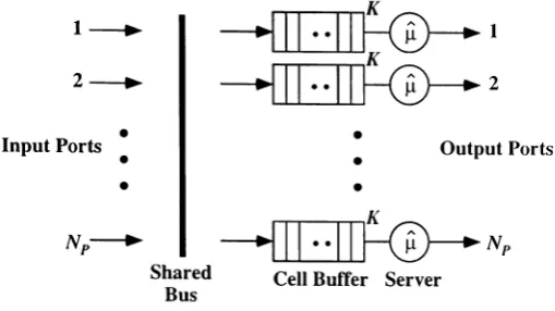
Figure 1: ATM switch architecture.

2.1

ATM Connection Traffic Descriptors

We characterize a connection requesting admission into the ATM network by the following

ATM connection traffic descriptors standardized by the ATM FOrUlTI User-Network Interface

Specification [1]:

~, peak cell rate (peR) in bps

"X,

sustained (average) cell rate (SCR) in bps

B,

maximum burst length in cells at the peak cell rate

(1)

(2)

(:3)

The (~,

X,

B)-triplet contains optional traffic connection descriptors which can be used to

derive the remaining required traffic connection descriptors that define the traffic contract,

specifically the cell delay variation and burst tolerance [1]. Each connection, which may be all

individual source or multiplexed sources, negotiates with the CAC~ algorithm for admission

into the network using these descriptors to describe the traffic.

2.2

ATM Sw-itch Architecture

The model for the ATM switch architecture considered here is shown ill Figure 1. TIle ATM

switch has Np input ports, and each connection in the network routed by the shared bus to

the output cell buffer of one of the

Np

output ports is described by the same

(~,

X,

B)-triplet.

Efficient Simulation of Cell Loss Probability.... , Freebersyser and Townsend

(~,K)

4

Connection Admission Control

YeslNo

Fig1lre 2: Connection admission control block diagram.

the shared bus during an arrival slot. The output cell buffers use a first-in, first-out

(FIFO)

queueing discipline. Each output cell buffer has a finite size of K cells, and cells exit the

output cell buffer at a service rate of

it

bps.

2.3

System Model

Our goal is to determine the cell loss probability due to buffer overflow resulting from the

worst-case conforming traffic conditions for a given set of ATM connection traffic descriptors

as a function of the number of connections in the network. We consider OI11y homogeneous

connection traffic in the network, that is, all No connections in the network which are being

routed through one of the Np output cell buffers of size K and service rate

p,

have identical

U,

X,

B)-triplets. The block diagram of the CAC algorithm for these conditions is shown in

Figure 2. We assume ergodicity in the traffic flow routed through each of the Np output cell

buffers, so that by examining one output cell buffer we obtain the performance characteristic

of all the Np output cell buffers, and that the output cell buffer is initially empty, since the

steady-state behavior of the system is equivalent whether it is reached by starting N

+

1

connections with an empty output cell buffer, or by adding an additional connection to the

existing N connections and a non-empty output cell buffer.

The worst-case arrival condition which is still compliant according to the Usage Parameter

Control (UPC) is when the traffic enters the network at the peak rate, A, such that the

worst-Efficient Simulation of Cell Loss Probability.... , Fvcebereyser and Townsend

A

B=4 cells

n-rT'l

T=16slots

~IIIIIIIIIIII

o

1 2 3 4 5 6 7 8 9 10 11 12 13 14 15

Figure 3: Busy /idle cycle example.

5

case arrival condition in determining whether or not a QoS measure for cell loss probability

is violated by admitting a new connection to the network.

We operate with a slotted-time system where an arrival slot is the amount of time that

one cell takes to arrive. The period of the busy/idle cycle of the arriving traffic,

T,

is the

time in slots that the

iJ

length cell burst at the peak rate must be averaged over so that the

sustained rate,

1,

is not exceeded, thus

T

==

iJ~/1,

slots (4)

An example of a burst of length B

==

4 cells is shown in Figure 3. TIle randomness ill the

system model described here is found in the connection starting-slot position. A connection

can start in any slot within the T length period, so we describe the connection starting-slot

position by a uniform probability density.

We let the number of ports on the ATM switch be equal to the number of connections

routed through the output cell buffer, Np

==

No, since this condition results in an upper

bound of the cell loss probability for any size switch, in terms of the number of input and

output ports. The data rate of the shared bus is then No cells per arrival slot, as shown

in Figure 4, so that all N

_c·

input ports have access to the shared bus in each arrival slot,

which results in N

_c·

service slots per arrival slot. When N

<

No input ports are active, we

make the worst-case assumption that the cells of the active ports occupy the first JV of No

service slots, rather than operating with some type of round-robin bus access mechanism.

We assume that each connection occupies every service slot position with equal probability

for each output cell buffer, so that the the cell loss probability for any one connection is

Efficient Simulation of Cell Loss Probability.... , Freebersyser and Townsend

Cell Arrivals

1

D

I Arrival

/ S l o t Service

D

Slot

2 I

/

1 2 N_c

•

•

•

•

•

•

Arrival Arrival

D

Slot Slot

N_c I Boundary Boundary

Figure 4: Relationship between arrival slots and service slots.

Check for

Arrival Blocks Departure

Service Slot Fill Service Service Slot

Boundary Buffer Boundary

Figure 5: Order of events within a service slot.

The effective service rate, u, of the server is

It

=

it

I

~,

cells per arri val slot

6

In each service slot, one cell can be loaded into the output cell buffer if there are arriving

cells and

/-lINe'

cells can be removed from the output cell buffer if the output cell buffer

contains greater than

/-lINe

cells. If the output cell buffer contains less than ItlN

_e

cells,

the available cells in the output cell buffer are serviced. If there are no cell arrivals, cells in

the output cell buffer are still removed according to this policy. Figure 5 shows the order of

events within a service slot.

While the ATM switch architecture considered here may seem simplistic more

corn-plicated ATM switch architectures can be considered using this methodology, TIle main

feature of this system model is that the traffic entering the network is defined in terms of

Efficient Simulation of Cell Loss Probability.... , Freebersyser and Townsend

3

Closed-Form Analysis of Cell Loss Probability

7

Consider the set V of all unique connection starting-slot vectors 'Q.I for j

=

1 ...

/VI.

A

connection starting-slot vector Qj is composed of N

_c

elements, where the l-th element ill the

vector represents the slot position, from slot 1 to slot

T,

where the l-th connection starts

its

13

length cell burst. Each connection starting-slot vector 'Qj corresponds to the loss of i

cells anel the arrival of l: cells in a steady-state period T

_{ss .}

Let n'_{C L l} be the total number

of connection starting-slot vectors 'Q.j that map to i cell losses in a steady-state period T

_{ss ,}

where

11/1

=

'Lf':oax

nCL , and Lm a x is the maximum number of cell losses in a steady-state

period

Tss.

The probability of i cell losses in a steady-state period

_Tss

is described by a

multinomial probability distribution with individual probabilities

(6)

h "\""Lmax 1

were LJi=O PCLl

== .

In a similar fashion, nC A k is the total number of connection starting-slot vectors Qj that

map to k cells arriving in a steady-state period T

_{ss .}

Thus,

11/1

==

'Lt~ox nC A k where Amax is

the maximum number of cells that can arrive in a steady-state period Tss . The proba.bility

of k cells arriving in a steady-state period T

ss

is described by a multinomial probability

distribution with indivi~ualprobabilities

h "\""Amax - 1

were LJi=O PCAk - •

Define the cell loss ratio (CLR) or cell loss probability, PCL' as

Total Number of Cell Losses 'L~oax in'C L l

PCL

==

T I N

_{ota urn er}

b

₀f Arri_rrivmg

C 11

_{e S} == "\""A_LJk=O

max

k_~n'CAk

(7)

(8)

We can also define PCL in terms of the average number of cell losses and the average number

of cells arrived, nCL and riCA' respectively.

1 ",L m a x .

iVT

LJi=O znC Li

PCL

==

~l----.;....",-A-m-ax-k-­

iVT

LJk=O nC A k

Efficient Simulation of Cell Loss Probability.... , Freebersyser and Townsend ₈

For the systems we consider here, we know that

n

C A is constant for a given

U,"X,

B)-triplet,

so we rewrite PCL as

- ~Lma.x •

f) _ n'C L _ L....,.i=O 'lPCLt

.LCL -

-nCA

n.,

(10)

Thus, PCL is a weighted sum of probabilities from the multinomial distribution of cell loss.

The variance of PCL is then

(11)

which will be used later in calculating the improvement in simulationefficiency,

The brute force method of determiningPCL is to sum the cell losses and cell arrivals over

the entire set

11

of connection starting-slot vectors 1?.j' A minor simplification is to fix 011e of

the connections at slot zero because the connection starting-slot vectors1?.jare translationly

invariant from this reference point, resulting in

where ICL is the binary indicator function of a cell loss in a service slot,

I.

== {

1, if a cell loss occurs

CL 0, if a cell loss does not occur

ICA is the binary indicator function of an arriving cell in a service slot,

{

I ,if a cell arrival occurs

lCA

=

0, if a cell arrival does not occur

(13)

(14)

T

_ss

is the steady-state period and has the same length as a period T, -il indexes the

starting-slot of the

i3

length cell burst of the l-th connection, and Ni- is the number of connections

routed through the output cell buffer. However, for even small values ofT and Ncr, the

Efficient Simulation of Cell Loss Probability.... ,Fteeoexeyscr eiu! Townsend

₉

4

Estimation Using Simulation

We first consider conventional MC estimation in a network framework. We then discuss how

the simulation itself is greatly simplified by the use of ATM connection traffic descriptors,

and show how IS is applied within this framework. We also derive upper and lower bounds

of the cell loss probability which can be used to determine if simulation of a particular set

of ATM connection traffic descriptors and switch parameters using this method is feasible.

Lastly, we consider some examples to demonstrate our methodology,

4.1

Monte Carlo

Sirnulation

The brute force method of determining PCL is intractable ifV is large, which is the case for

many realistic systems of interest, so we use MC simulation to estimate PCL by randomly

selecting

N

D of the starting-slot vectors 12.jout of

V

and form the estimate

PCL

" 1 x-No ~Tss~Nc I (' , )

p. _

nC L _ N;;L..."i=l L..."j=l L..."n=l CL Z,J,n

CL - " - } ~Nn ~Tss ~Nc I (' , )

nCA Nn wi=1 wj=1 wn=1 CA 'l,J,n

(15)

We can rewrite (15) using the multivalued indicator function ofa cell loss for all No

connec-tions in a steady-state period

Tss

M _ { L, if L cell losses occur for 1

<

L

<

Lm a x CL - 0, if a cell loss does not occur

(16)

and the multivalued indicator function of a cell arrival for all No connectionsin a steady-state

period

Tss

MC A

= {

A, if A cell arrivals occur for 1

<

A

<

Am a x

0, if a cell arrival does not occur

(17)

(18)

as

" } ~Nn M (')

" nCL N;;wi=} CL 'l

PCL == -"- == 1 No 7\{/ (')

n C A Nn Ei=l.1Vj CA i

where M_{C L} and M_{C A} map each starting-slot vector 12.j drawn independently from

11

to L

cell losses and A cell arrivals, respectively, in a steady-state period T

ss .

The multivalued

indicators functions are used instead of the binary indicator functions ill order to obtain

Efficient Simulation of Cell Loss Probability.... , Freebersyser and Townsend 10

(20)

a cell loss results ill a correlated binomial distribution because the cell losses are the result

of bursty events [13].

Since all No connections generate a burst of length

iJ

cells, the number of arrivals per

steady-state period

_Tss

is

1 (

A)

A

nCA

=

N

D

NDNc B

=

NcB

(19)

As mentioned previously.,

n

C A is constant so we are actually concerned with estimating nCL,

the numerator in (15), the average number of cell losses per steady-state periocl T

_{ss .}

By

estimating nCL we are implicitly estimating the PCLi of the multinomial distribution of cell

loss.

In order to determine the confidence interval of PCL' the

Me

simulation V\Te consider

actually estimates nCL and therefore PCL by independently drawing Ns of NR connection

starting-slot vectors 12jout of the set V.

1 " Ns " NR M (' ')

n _

~ ~i=l ~j=l cL'l,]

TCL - _

nCA

We determine the confidence interval of PCL by letting the estimate of PCL corresponding to

the i-th of N

_s

sets of

NR

independent draws be PCLt' where i == 1., ... ,N

s .,

so that overall

estimate of PCL is the sample mean

A 1 Ns A

PCL

=

N

2:

PCL,

S i=l

(21)

(22)

We estimate the variance of PCL by the sample variance

I N s

&2

(P

C L )

=

N (N _

1)

2:(P

C L ; -

p

C L)2 S S t=l

We do not assume a normal distribution for the confidence interval, but use the method

found in

[14],

which determined that the confidence interval of a weighted sum of individual

multinomial probabilities follows a X2 _{distribution. We state the theorem from}

_[14]

_{with the}

original notation slightly altered for our application:

Theorem: As

NsN

_R --+ 00, the lower limit of the probability that PCL satisfies

Efficient Simulation of Cell Loss Probability.... ,Fteebersyser and Townsend 11

is at least 1-a where A is tile positive square root of the upper (1 - a)-th percentage point

of the \,2 distribution with Lm a x degrees of freedom.

The multinomial framework used here reduces to the more familiar binomial case with

normally distributed confidence intervals when Lm ax

==

1. lJsing the \2 distribution results

in wider confidence intervals than using the normal distribution, but because we have used

the multivalued indicator functions in

(18)

rather than the binary inclicator function in (1,5),

we have independence between cell loss events. This is critical since cell loss events occur

in a bursty fashion, which makes tile binomial random variable represented by the binary

indicator function correlated [13]. Measuring this correlation is difficult when rare events

are involved, which in turn makes deriving accurate confidence intervals of our estimates

difficult. This problem is solved by the multinomial framework because the selection of each

connection starting-slot vector 12-j from

V

is done independently.

4.2

Monte Carlo Simulation Framework

As stated previously, the randomness in the system model is found in the position of the

connection starting-slots. Once the connection starting-slot vector 'Qj has been drawn, the

system model behaves deterministically in that the number of cell arrivals a.s well as the

number of cells serviced is known for each slot.

By observing the performance of this system, several characteristics were determined that

assist us in speeding up the simulation without applying IS. First, we are working with a

stable system since the size of the output cell buffer is finite. Second, we are able to detect

the onset of tile steady-state. Last and most important, the system exhibits predictable

behavior in the mechanism that causes cell losses, so we can anticipate if a cell loss is going

to occur for a given connection starting-slot vector 12-j. We need only observe the queue

length for three periods to determine whether or not a cell loss OCellI'S. We use the following

rules to take advantage of these three characteristics:

Define X

[n]

as the queue length in cells and A

[n]

as the number of arrivals in cells at the

Efficient Siinuleiion ofCell Loss Probability.... , Freebetsyset and Townsend

Nc

=

3 connections

12

A.

B=4 cells _{t---+--+---I--I}

T=16slots

o

1 2 3 4 5 6 7 8 9 10 11 12 13 14 15

Figure 6: Aligned at zero example.

1. The cell arrivals that occur during the 2nd period constitute the steady-state cell

arrivals, i.e. A [T

+

n,]

=

A[h~T

+

T

+

n]

where k is a non-negative integer.

2. If the output cell buffer size remains unchanged from the end of the second period to the

end of the third period,

4X"

[2T]

=

4X"

[3T],and a cell loss does not occur, l\,tC L (2T~ 3T)

==

0, the steady-state has been reached and a cell loss will never occur for this particular

connection starting-slot vector 12j.

3. If the output cell buffer size increases from the end of the second period to the end of

the third period, 4\"[2T]

<

X [3T], the output cell buffer size keeps increasing until a

cell loss occurs.

4. When a cell loss occurs in a period,

M

C L

(kT, (k

+

1

)T)

>

0 for

k

~ 2,

k

an integer,

and the output cell buffer size at the end of consecutive periods is the same, ~\ [h~T]

==

..X"

[(k

+

I)T], the steady-state has been reached.

The connection starting-slot vector12j that results in the maximum number of cell losses

in a period corresponds to the situation where all the connections start at slot zero, which

we define as the aligned at zero (AAZ) case as shown in Figure 6. The maximum number of

cell losses that can occur in a steady-state period T

ss ,

Lm a x , is then

L

m a x =

l

i3

(N

c - It) -

I{

J

+

1 (24)

We will consider two types of cell losses: Type A and Type B. Type A cell losses occur

Efficient Simulation of Cell Loss Probabili(y.... , Freebersvse: and Townsend

arriving cells over a timet

<

T

and an output cell buffer overflow results in a cell loss. Type

B cell losses occur when the total number of arriving cells in a period T is greater than the

service available. We will be mostly interested in Type Acell losses since such cell losses are

rare events.

Type A cell losses can not occur until there is a sufficient number of arriving cells over a

given time window. Since all arrival must occur for a cell loss to occur, we assume the AAZ

case to get the worst-case conditions for cell loss, that is the least number of connections

that result in a cell loss requires that

A A

EN

c

>

1< +Bf.1

Thus the minimum number of connections, Nc m in , required to cause a cell loss is

(2,5)

(26)

where

r

x

1

is the ceiling operation that rounds x up to the next highest integer if x is not all integer. For a number of connections Nc

<

Nc m in , cell losses at the output cell buffer can

never occur.

Type B cell losses, where a cell loss is guaranteed a priori, occur when the SUIll of the

average rates of all the connections is greater than the available service, or

f.1

<

AN

c

(27)

Therefore, the number of connections, N_cg, required to guarantee a. cell loss at the output

cell buffer is

(28)

The performance region we are interested in is over the range of connections lVc m i n :::;

NCf ::; NCf_g• However, when cell losses are rare events, which is oftell the case in realistic

systems of interest,

Me

simulation is slow, therefore we use IS to make the simulation more

Efficient Simulation of Cfell Loss Probability.... , Freebersyser and Townsencl

4.3

Efficient Simulation Using Importance Sampling

14

.

The basic notion behind IS is to modify or bias the original proba.bility density function for

the connection st.art.ing-slot vector,

i-

(v),

to a new proba.bility density function, j'~(v), that

reduces the variance of the estimate of PCL' while weighting ea.ch cell loss event so that P~L

remains an unbiased estimate of PCL. The only required condition on the pdf ~f~(v) is that

f;(v)

>

0 when the multi valued indicator function .MC L

(Qj

E

VCL)

>

0, where

VCL

C V is

the subset of connections starting-slot vectors which cause a cell loss. The pdf .fv(v) we

consider here is the product of i.i.d. uniform probability density functions.

The key to using IS is knowing how to bias the pdf fv(v). Intuitively. we want to use

IS to increase the number of cell losses that occur. Type B cell losses result ill high va.lues

for PCL' so vee are most interested in Type A cell losses. We have previously determined

that the connection starting-slot has a uniform probability distribution over a period

T.

Unfortunately, there is no general bias scheme for the uniform probability distribution known

to the authors that is effective.

4.3.1 Theory

For this problem, we use a priori information about the system 1110del to determine an

effective bias scheme. The approach we take is based on the idea that one connection is fixed

to start at slot zero and an examination of the restrictions involved with using IS. Assume

we know the set VCL of connection starting-slot vectors'Qj that cause cell losses. Then PCL is

(.1)

Nc-1 '\'I,vC LI1\,{ (i )

T L...,,1.=1 CL

PCL

==

"-NcB

(29)

IS is applied by reducing the set of connection starting-slot vectors

u,

from

I\/ I

to

1'-''"* I

<

Il/

I

such that all of the non-zero cell loss events are included in V", i.e. \/~L C ll* C l/. This

results in n~LJ

=

nCLl for i

=

1 ... Lm a x , which implies that n'~LO

<

n'CLo· By maintaining

all the connection starting-slot vectors that cause cell losses in ll*, we do not violate the

Efficient Simulation of Cell Loss Probability.... , Freebersyser a,nd Townsend

like VCL = V*, but as long as IV*I

<<

IVI and VCL C V*, the efficiency of the simulation can be increased.

This reduction in connection starting-slot vectors results in the biased individual

proba-bilities from the multinomial distribution for cell loss

(:30 )

The relationship between the unbiased PCL, and the biased P~L, is based on the the weight

function or likelihood ratio, ltV

==

IV* I/IVI,

so that

(:31 )

Therefore, IS implicitly biases the PCLi to P~Li'

The cell loss probability found using IS, P;L' is the same as that found without using IS.

The variance of P;L is

Lm a x

(iW)

2 * _ t.;ax

(il/I!)

')*

L -

PCLi

L -

1ci.,

i=O nCA i=O n'CA

L

m a x

( i ) 2 L

m a x ( i )

W

L

=--

PCLl -

L

=--

]JC L l

i=O n C A i=O n C A

(33)

which will be used later in calculating the improvement in simulation efficiency.

4.3.2

Application

We mentioned previously that Type A cell losses occur when individual connections start so

close together that the server can not keep up with the arriving cells over a time t

<

T

and

an output cell buffer overflow results in a cell loss. Assume that one connection is fixed to

start at slot zero. Then for a given number of connections, we can determine the distance

in slots c from the connection fixed to start at slot zero, so that a cell loss does 110t occur

Efficient Simulation of Cell Loss Probability....~ Fteebersvser a.nd Townsend 16

multi-valued indicator function l\le L is always zero outside this region and the support of the

uniform pdf that originally covered the entire interval T can be reduced around both sides

of slot zero.

Define Cmin as the distance in slots from the start of the 13 length ('('ll burst of the

connection furthest from slot zero for a connection sl.arting-slot vector 12.1 that still causes

a cell loss for NC'min connections, and define C m in+l similarly for NC:rllin+l connections.

TIle

equations used to determine Cmin and C m in+l are a function of the

ATIVI

connection traffic

descriptors and the switch parameters.

For J.l

2:

1.0 and

Nc.: -

1

<

J.l

~ K

emin

=

LB - 1'1 J

+

1

Cmin - It

A ! { _

unless

B -

N _

==

0 then Cmin - 0, and

Gmin J..L

C min+l ==

B

+

Cmin

For J.l

2:

1.0 and

NCf

m in - 1~

J-l

unless

B

( N_{C m in} -

J-l) - ]{

== 0 then Cmin == 0, and

C min+l ==

B

+

Cmin

For J.l

<

1.0

Cmin ==

l

B/

It -

B

J

+

1

and

C min+l ==

l2B/J-l- B

J

+

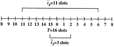
1

The number of slots covered by the biased uniform pdf is

i

==

2c

+

1

(34)

(:35 )

(37)

(:38 )

(39)

Efficient Simulation of Cell Loss Probabili(y.... ,Fteebersyee: and Townsend

I I I I I I I I I I I I I I I

8 9 10 11 12 13 14 15 0 1 2 3 4 5 6 7 8

T=16slots I

~=3slots

Figure 7: Example of

i

distances.

17

compared to the unbiased uniform pdf that covers the full T slot period. An example of

i

slot distances is shown in Figure 7.

This quasi-analytic form of IS fixes the weight within the simulation according to how

much the support of the original uniform pdf is reduced around the connection fixed to start

at slot zero. Each connection starting-slot 1!..j is drawn independently from the identical

biased uniform distribution, which results in the weight function

Nc

II

("

)NC-I

vV

=

I

v (

v)/

I~

(

v)

=

I

j (

v)/

I](

v)

=

t /

T

j=2

(41)

The expression of the weight function in

(41)

is the same as that in (31) where

11/

1= TNc-I

and IV*

I

=

iNc-I.

4.3.3 Simulation Using IS

The

Me

simulation using IS estimates P;L by independently drawing N s sets of NR

connec-tion starting-slot vectors 1!..j out of the set V*

1 \:"'Ns \:"'NR M* (. ,.)

" N sNR L--i=I L--j=I CL 1" J

P~L = - - - - = : : - - - - = - : : . . - - - (42)

where M~L(i,j)takes on the values 1 to Lm a x and indicates the number of cell losses for the

(i,j)-th connection starting-slot vector Qj drawn from the biased distribution, .f;(v).

Now for

NCmin'

we observe that PCL

(NCmiJ

=

PCL

(imin) ,

but for PCL

(NCmill+l)

this is not

the case. Rather we have

Efficient Simulation of Cell Loss Probability.... , Freebersyser tuu! Townsend ₁₈

We first find the cell losses involving the connection fixed at zero, or N_{C L}

(imin+1),

and then add in the cell losses not involving the connection fixed at zero, N_{C L}

(i~in+1)'

We account for the cell losses outside the

t

m in+1 range by sliding the

f

m in range over the T -

t..lIn+1

slots outside

t

m in+1 and subtracting the AAZ case at the boundary so that

NC L

(imin+1)

+

C~~:ii:+l

(T -

L.in+1)

N_{C L} (NCmiJ

+

N

C L

(N

C m in ) -

N

C L

(N

C m in AAZ) (44)

N c .

where

eN

_Cmin'mm+l ==

N

_C'min+l is the combination operator and this factor accounts for the

different combinations of

NCf

m in connections that can occur outside the

i

m i n+1 range. We

divide by a factor of

l/T

N

cm in + l-1 and use

(44)

to find

(45)

or in terms of PCL we have

(46)

(47)

which is a very tight bound since the AAZ case constitutes such asmall portion of the total

number of cell losses. In finding PCL

(N

Gmin+l)'

we actually violate the IS rule that

.f~

(

v)

>

0

when

M

C L

(Qj

E

V

C L )

>

0 in a known way, and correct for this by replacing the correct

number of cell losses using PCL

(N

GmiJ·

The simulation uses the estimates of PeL

(L.IO+l)

and PeL(N

Gmin)

to estimate PCL (N

Gmin+l)

in

(4

7).

The variance of P~L

(N

C m in ) is the sample variance

Efficient Simulation of Cell Loss Probability.... , FreebersJ!ser and Townsend ₁₉

The variance of

P~L

(N

G'min+l)

is the weighted sum of the variances

;;-2

(P~L

(fmin))

and

;;-2

(P~L

(imin+l))

;;-2

(P~L

(NGmin+l))

+

The quantities in (48) and (49) are used in the calculation of the confidence intervals of the

estimates for

P~L

(N

GmiJ

and

P~L

(N

Gmin+! )

4.3.4 Calculation of the Improvement Factor

The improvement,

_Rnet,

that results from using IS describes the factor by which an IS

estimator that uses the given method is more accurate than a conventional IVI C estimator

based on the same sample size, or, equivalently, how many fewer steady-state periods must

be simulated to obtain a given accuracy. The improvement,

Rnet,

is found analytically by

taking the ratio of the variances, (J2 (PCL) and (J2 (P;L) from (11) and (3:3), respectively.

L

(

. )2

. max _~_ _

p2

L~=o riCA PCLI CL

L

(

. )2

W .max ~ _

p2

Lz=o

nCA PCLt CL

1

--+ - as PCL --+ 0

l¥

(50)

As PeL ~ 0, the improvement obtained by using IS approaches the inverse of the weight

from above, so a lower bound on the improvement,

l

RnetJ,

is

(

,,)NC-l

l

RnetJ

== l/vV == T

[t

(51)

From (51), we see that improvement always results if

i

<

T

for any value of PeL if Nc

>

2.

4.4

Upper and Lower Bounds of the Cell Loss Probability

The distance Cmin can be used to derive an upper bound for PCL for N_{C m in} connections by

assuming that L_{m a x} cell losses from (24) occur whenever one or more cell losses occur. For at

least one cell loss to occur, all NC m i n connections must start within Cmin slots of each other.

Efficient Simula.tion of Cel! Loss Proba.bility.... ,Fteeberevser and Townsend

₂₀

Figure 7).

If

we assume that one connection is fixed at slot zero, the probability of the remaining NC min - 1 connections starting within Cmin slots of each other is (Cmin/T)NCmin-1.

Therefore an upper bound for PCL is

n'C A

P

(a11Y cell loss) Lm a x

n'C A

NcminE

For the experimental systems considered later, the upper bound in (52) is one or two orders

of magnitude high.

An upper bound for PCL for NCmin+l connections can be derived using the same method

used to find the PCL

(NCmin+l)

in (47), except that we substitute the bounds for PCL

(LlIl+1)

and PCL

(i~In+I)

into (47) rather than the estimates. We upper bound PCL

(imin+1)

using

(52)

as

nCA

p (any cell loss)Lm a x

n

C A

(~

)NCmin+l -1

(C

_min+1

+

1)

(l

iJ

(NCmin+l -

It) -

I\

J

+

1)

We use

r

PCL

(NCmin)l

in the expression for PCL

(i~in+1)

so that

PCL

(NCmin+l)

<

r

PCL (

NCmin+l )l

r

PCL

(imin+1)

1

+

r

PCL

(i~m+1)

1

r

PCL

(t

min

+

1 )

1

N

C min

(Ncmin+l

(T -

t

min

+

1)

+

1)

flJ

(N-,)1 (54)

+

N T CL Cm lO

Cm in + l

A lower bound for PCL for a number of connections less than that guaranteed to cause an

error,

Nc

<

Nc

Efficient Simulation of Cell Loss Probability.... , Freebersyser eiu! Townsend ₂₁

(S,5 )

case shown in Figure 6, where Lm a x cell losses occur. If we aSSUTIle that one connection is

fixed at slot zero, the probability of the remaining

No -

1connections starting at slot zero,

is (l/T)NC-l. Therefore, a lower bound for PeL is

(

)NC-1( "

)

lPeL(No<Ncg)J=l~ed= ~

lB(Nc,-p)-AoJ+l

n'C A Nc.,B

For combinations of

(~,

X,

B)-triplets and

(fl,

K)-pairs that result in C

_min

=

0, the lower

bound is exactly PCL for N

_Cmin

connections.

A lower bound for PCL for a number of connections greater than or equal to that

guaran-teed to cause an error, lVe

2:

Ncg,is found by assuming that for every connection starting-slot

vector 12.j, the Lg cell losses associated with the overflow ill a period T occur so that

(56)

where

L'g

==

n

C A -

ItT.

This is a lower bound because it is possible to lose more than

Lg

cells, such as in the AAZ case where Lg ::; Lm a x • In (56), we also see that as N

c

increases,

PCL ~ 1as expected.

4.5

Feasibility of System Simulation

We can determine whether or not a given system can be simulated effectively before

SilTIU-lation by using the upper bound of PCL and the lower bound of

R

_{n e t •} We define

PCL

as the

equivalent cell loss probability that must be simulated using conventional

Me

simulation

after the improvement has been taken into account. We will see later that the upper bound

of PCL(N

c m in) is roughly two orders of magnitude high for the experimental examples vve

consider here, so to find

PCL

we divide

r

PCL

(Ncmin)l

by a factor of 100as in (S7)

(

T ) Nc . -1

PedNomiJ

=

(fPedNomiJl

/100)

i

min

rrn n

We define the simulation effort, E, as

E ==

TNc/P

c L

(,57)

(,58)

noting that the effort required by any simulation is inversely proportional to PCL and

1)ro-portional to

T

and

Nc.

Based on the results of the experimental examples vee consider later,

Efficient Simulation of Cell Loss Probability.... , Freebersyser and Townsend 22

System j, Mbps

X,

Mbps B, cells u. Mbps 1\, cells

01 500 50 2 200 4

02 8 2 4 1:3 !)

Table 1: ATM connection traffic descriptors and switch parameters for the simple examples.

System T, slots p.,cells/slot N_{C m in ,}corms. _Cmin' slots Lm a x (Nc . ),rru n cells

D1 20 0.8 3 1 1

02 16 1.625 3 1 2

Table 2: Derived simulation parameters for the simple exa.mples.

4.6

Sjrnulat.ion

Methodology

In order to demonstrate and verify our methodology, we considered the two simple examples

with the ATM connection traffic descriptors and switch parameters given in Table 1. The

parameters for the simple examples were selected so that the PCL a.nd PeLt could be

deter-mined by brute force as in (12). The service rates were selected so that the different formulas

for determining Cmin and Cmin+l could be tested depending on whether fJ

2:

1or 1.£

<

1.

The ATM connection traffic descriptors and switch parameters in Table 1 are substituted

into the appropriate equations in Section 4.3.2 to find the derived simulation parameters for

the simple examples shown in Table 2. The derived simulation parameters are used as inputs

to the simulation.

The exact results for NC'min and NC'm in + l connections for the simple examples are shown

in Table 3. We performed conventional

Me

simulation and simulation using IS for N Cmin

and N

_{e .}

connections using N

s

=

20 of NR steady-state periods shown in Table :3 ill

m in-l-l

order to compare MC and IS simulation results. The estimates of PeL from the MC and

01 3 10,000 2.917 X 10-3

D1 4 10,000 9.975 X 10-3 02 3 40,000 2.604x 10-':3 D2 4 40,000 1.811X 10-£J

System ~ Nc, conns. I NR PCL

Efficient Sunuleiiou of Cell Loss Probability.... , Freebersyseteru! Townsend 23

95~ CI

95%CI _CL 0

Dl 3 2.956X10 '0 (2.850X 10 '0,3.062X10 '0) 2.915X10-'- (2.B08x10-:\ 2.922X10"":3) Dl 4 9.975X10 -0 (9.773X10 '0 11.022X10 .:L) 9.981X10 -3 (9.941X10-'J,1.004X10-2₎

D2 3 2.621X10 ~ (2.578X 10 '3,2.666X 10 .3) 2.604X10-,-0 (2.GOUx 10-:\ 2.f)USx 10-3 )

D2 4 1.827X10 .'2 (1.795X10 .J,1.859X10 .3) 1.814X10 ·2 (1.7~J;-': X 10-3_{, 1 .8 :12x 10--:3)}

System INc,conns.

II

Table 4: lVIC and IS estimates and confidence intervals for the simple e-xamples.

Exact Observed l/W Exact Observed l/Hl

I

I

System Rn e t NCm 1ll ti.; NCrnin for NCmin

«:

NC mi n 4- 1 Rn e t NCmin+l for N('TfIIf1+1

Dl 196.5 226.0 44.4 26.0 23.7 11.0

D2 96.0 123.7 28.4 4.3 4.0 3.1

Table ,5: Improvements for the simple examples.

IS simulations and the resulting confidence intervals of the simple examples are S110\Vn in

Table 4. Confidence intervals for the estimates of PCL for N_{C m i n} and N_{C rn m}+₁ connections

are determined using the method from

[14]

given in (23). As expected, the estimates of PCL

found using IS are closer to the exact value for PCL than the

Me

estimates, and also have

tighter confidence intervals.

Shown in Table ,5 are the improvement factors obtained for the simple examples using

several different methods. The exact improvement is found by substituting the PCL, found

by brute force into

(.50).

The observed improvement is found by taking the ratio of 0-2

(P

C L ) and &2 (P~L) since the Me and IS simulations were performed for an identical number of NR

steady-state periods. Finally, the value of l/W is given, and this quantity is indeed a lower

bound for R_{n e t}• Clearly, the computational effort expended in estimating PCL by simulation

for the simple examples is greater than that required by brute force, but the purpose of this

exercise was to verify the methodology itself rather than estimate PCL'

5

Experimental Examples

We considered the following experimental examples, where PCL and ]JCL, are unknown, with

the ATM connection traffic descriptors and switch parameters shown in Table 6. The derived

simulation parameters for the experimental examples are shown in Table 7. The cell loss

Efficient Simulation of Cell Loss Probability.... , Freebersyser a.nd Townsend

System ,,\, Mbps X, Mbps

iJ,

cells I'·, Mbps tc,cells

1 15 1 10 120 100

2 15 1 200 120 100

3 50 1 10 120 100

4 50 1 200 120 100

5 75 1 200 120 100

6 15 5 25 120 100

7 50 5 25 120 100

8 500 2 10 120 200

9 500 10 25 120 200

10 500 1 100 120 200

11 500 2 50 120 200

12 500 2 100 120 200

13 2.1 0.031 148 120 100

14 32 1 200 120 100

24

Table 6: ATNI connection traffic descriptors and switch parameters for the experimental

examples.

System T, slots u, cells/slot NCmin' conns. Cmin,slots _Lm a x(Nc'm"n)' cells

1 150 8.0 18 0 1

2 3000 8.0 9 101 101

3 500 2.4 13 7 7

4 10000 2.4 3 34 21

.5 1.5000 1.6 3 129 181

6 75 8.0 12 0 1

7 250 2.4 7 15 16

8 2500 0.24 21 32 8

9 1250 0.24 9 80 20

10 .50000 0.24 3 317 77

11 12500 0.24 5 159 ;3~)

12 25000 0.24 3 317 77

13 10025 57 1/7 58 32 '27

14 6400 3.75 5 121 _I 151

Efficiellt Simulation of C~ellLoss Probability.... , Fteebcrsvse; tuu! Townsend

Nc ,conus. PCL Comment

120 1.38x 10-~ e

=

0.02 110 1.96 x 10-3

( =

_0.04

100 2.49x 10-4

f

=

0.1

90 2.08x 10-5

f

=

0.2~)

80 2.03x 10-6

( =

_0.2

19 3.92 x 10-~" Upper Bound

18 5.64x 10-4u _Exact

17 0 Exact

Table S: Cell loss probability as a function of the number of connections for system 1.

Nc, conns.

PCL

COn1111ent

120 2.10x 10-2 _e

=

_0.02

110 3.68 x 10-3 _{( = 0.07}

100 5.50 x 10-4 _{e= 0.10}

90 6.78 x10-5

f

=

0.12

80 7.36 x10-6

f

=

0.10

14 7.17x10-2 0 _{Upper Bound}

13 2.88x10-24 _{Upper Bound}

11 0 Exact

Table 9: Cell loss probability as a function of the number of connections for system :3.

8-16. The estimates of PCL for systems 1, 3, 8, and 13are shown i11 tables because vve were

unable to generate complete performance curves for reasons whichvee discuss later. However,

PCL for these systems is extremely low and in such systems we give the upper bound. For

systems 1 and 6~ we are able to determine the exact PCL using the lower bound in (5.5) since

Cmin

==

0, which results in L_{m a x}

==

1cell losses for the AAZ case for NC m in connections. Note

that a PCL ~ 10-14 corresponds to 1 cell loss per year for a service rate on the order of 1

Gbps.

Nc, conns. PCL C~0111ment

61 1.64x 10-~ Exact

60 1.96X 10-3 c= 0.01

22 4.84 x10-3 2 _{Upper Bound}

21 1.75x 10-3 8 _{Upper Bound}

20 0 Exact

Efficient Simulation of Cel! Loss Proba.bility.... , Freebersyser and Towuncni! By.tem 2 26 1xlO-1. lxlO-:l lx10 -3 lxlO -4 1x10 -5

..:I 1x10 -6

(£10u

-7 lx10 1x10 -8 1x10 -9 lx10-1 O lx10-1 1 lx10 -12 lx10 -13

---)..---~

~..---. /V

VV

/

0 20 30 40 50 60 70 80 90 100 110 12 Number of connect ions

Figure 8: Cell loss probability as a function of the number of connections for system 2 (TIle dashed portion of the curve is a straight line interpolation).

lxlO -1 -2 lx10 1x10 -3 ..:I (£10U -6 lxlO lx10 -5 1x10-b -7 1x10

----

--- I.---~ ~---V V

V

/ '

)

/

J

I

f

I

10 20 30 40 50 60 70 80 90 100 110 120 Numberotconnections

Efficient Simulation of Cell Loss Probability.... , Freebersyser a.nd Townsend

₂₇

lx10 -1 -2 1x10 -4 lxlO ~

---

,..---

---~ /

",,-...-' /

~

/

v

v

/

,

I

10 20 30 40 50 60 70 80 90 100 110 120 Number of connections

Figure 10: Cell loss probability as a function of the number of connections for system ,5.

System 6 -~ lx10 -2 lxl0 1xl0-3 -4 lxlO -5 lxl0 1xl0 -6 -7 lxl0 -8 lxlO 1x10 -9 -10 lxl0 -11 lxl0 -12 lxl0 -13 lx10 -14 lx10 lxl0 -15 -16 lxlO -17 lxl0 -18 lxl0 -19 lxl0 -20 lxl0 -21 lxl0 -22 lxl0 -23 lxl0 -24 lxl0 ~

---~ »> / V

10 14 16 18 20 22 24 26

Number of connections

Efficient Simulation of Cell Loss Probability.... , Freebers,yser and Townsend System 7 28 1x10 -1 1x10 -2 lx10 -3 1x10 -4 1x10 -5 ..:I u (QI 1x10 -6 -7 lx10 lx10 -8 lx10-9 1xlO-1 O

v

V

/

~

/

V

/ /

/

/

/

/

f

t

10 12 14 16 18 20 22 24 26 28 Number of connections

Figure 12: Cell loss probability as a function of the number of connections for system 7.

System 9 lx10 -1 1xlO-2 -3 1xlO -4 lx10 ..:I lx10-5 (QIu lx10-6 lx10-7 lx10 -8 lx10 -9 1.x10-1 O -11 1.x10 ~~ ,...

/

,

J

/

/ '

/

I

/

/

8 10 11 12 13 14 15 1

Number of connect 10n8

Efficient Simulatiol1

of

Cel! Loss Probability.... , Freebersyser and TOlvnsend

System 10

29

lx10-2

lx10 -3

~I.--""" ~

~

,....---:

~

~V

V

V

I

If

J

I

0 10 20 30 40 50 60 70 80 90 100 110 12

~

Number of connections

Figure 14: Cell loss probability as a function of the number of connections for system 10.

System 11 -1

lx10 lx10-~

lx10 -3 -4 lxl0

..:I

<AeU 1x10 -5 1xl0-6 -7 1x10 lxl0-1t 1x10-9

~

.----~~

V

~

. /

/

V

/

V

/

(

10 15 20 25 30 35 40 45 50 55 60 Number of connections

Efficient Simulation of Cell Loss Probability.... , Freebersyser and Townsend

System 12

lx10-J

~

---'

/ ~

/

~

V

/

V

9 I

~

~

10 15 20 25 30 35 40 45 50 55 60 Number of connections

Figure 16: Cell loss probability as a function of the number of connections for system 12 (The dashed portion of the curve is a cubic spline interpolation).

Nc, conns.

PeL

Comment

3870 4.91 x 10-~ f

=

0.01

3500 1.57x 10-2 _e

=

_0.04

3200 4.47 x 10-3

f

=

0.05

2900 7.11 x 10-4

e

=

0.14 2600 6.96 x 10-5

f

=

0.:37

2400 6.56 x 10-6

c

=

0.:30 2200 4.22 x 10-' c

=

1.00

59 2.01 x 10-10 1 _{Upper Bound}

58 5.60 x 10-14 4 _{Upper Bound}

57 0 Exact

Efficiellt Simulation of Cell Loss Probability.... , Fteebcvevsev «ud Townsend

System 14

:31

1x10-1

1x10-~ 1x10 -3

..:I

(~u 1x10 -6

1x10 -5 lx10 -6 -7 1x10 lx10 -8

-

~

....--

,;-.-~~

. /

V

V

/

)

/1

9

10 20 30 40 50 60 70 80 90 100 110 120 Number of connections

Figure 17: Cell loss probability as a function of the number of connections for system 14 (The dashed portion of the curve is a cubic spline interpolation).

For each performance curve, the bottom two points were obtained by simulation using

IS, and the remaining points were obtained by conventional lVrC simulation. The accuracy

of the Me; estimates is measured using the precision, E, which we define as

0-

(PeL)

E=

-"';""",,--PCL

(59)

and is typically E

S

0.1 for the systems where performance curves could be obtained.

Two types of discontinuities occur in the performance curves. In (26), we determined

the minimum number of connections, NCmin' needed for at least one cell loss at the output

cell buffer due to overflow. Thus, for N

_c'

<

NCf_{m in ,} PCL

==

O. TIle downward pointing arrow

at the bottom of each performance curve is meant to signify that PCL is zero below N_{C m in}

connections, thus there is a point on the performance curve where cell losses begin to occur

and below this point cell losses do not occur. This is an important result because the C~AC

algorithm can quickly determine that a new connection can be admitted to the network since

Efficient Suiniuuion

of

elfell Loss Proba.bili(y.... , Fteebereyeer eiu! Towiiseiid :32

System PCL (Nc . )rm n 95%CI NR PCL (Ncmin+l) 95%) CI NR

2 1.00X10 13

(7.55X 10 14

I1.25X10 1~\) 4000 2.09X10 1:2 (0.0,{),41 X 10-1 2 ) 20000

3 NS NS

4 4.75X10 7 _{3.G8

X10 (

,5.83X 10 I) 20 3.25X10 .(j _(1.G4 Xnr",4.87Xur") 40 5 4.36X10 ·5 (:).2:) ~ lOb15 .3 9X10 '5) 50 1.31X10 4 _{(8.88X10-'.1,1.7:3X10-}4

) .sO

6 7.89X10 ·:24 _{CFS NS}

7 4.61 X10 10 _{(:L~.C)X 10}

"'. 5.36X10 lU) 10000 1.85X10 8 (8.:~~)X10-::1,2.:-)(; / 10-8) 10000

8 NS NS

9 2.96X 10 ·11 (2.09X10 '11,3.84 X 10 11) 1000 6.09X10 ·9 (1.~J5X10-9,1.02 _{/ 10-~) 1000}

10 1.01 X10 ·5 (5.3,5X10 '6,1.49X10 .5) 20 3.01 X 10-;.) (LOSX 10-.1,4.9R X 10-'s ) SO

11 4.23X10 ~ _{(3.83X 10 .~,4.63}X10 .~) 1000 2.70X 10 ·4 (2.39X 10-8_{,3.UOX 10-~) 1000}

12 4.06X 10 ·5 (3.30X 10 J,4.82X 10 5) 200 1.27X10 ·4 (9.36>~ 10-'.1, 1.(iUX 10-1_{) 200}

13 NS NS

14 3.18X 10 ·8 (1.07X 10 '8,5.29X 10 .8) 50 1.68X10 ·8 (2.59X lU-~,3.10X 10-8 ) 100

Table 12: IS estimates and confidence intervals for the experimental examples(C~FS

==

Closed

Form Solution, NS

==

Not Simulated).

The guaranteed cell loss condition in (28) also creates a discontinuity in that there is a

point on the curve where a 'jump' in the cell loss probability is possible. TIle discontinuity

related to the load being greater than the available service is only noticeable for system 9

in Figure 13, where we see a 'jump' of 5 orders of magnitude in

PCL

between

Nc:

=

12 and

N_e.

==

13 connections which is associated with the guaranteed cell loss floor that begins at

No

==

1:3 connections.

Confidence intervals for the estimates of PeL for N Cmin and NCmin+l connections for the

experimental examples using the method from [14] given in (2:3) are shown in Table 12.

Because the experimental examples we considered are capable of large values for the degrees

of freedom,

L

_{m m} the \'2 distribution can give negative values for the lower confidence interval,

such as in system 2. In such cases, we use zero as the lower confidence interval.

For systems2,6, 12, and 14 in Figures 8,11, 16, and 17, the use of this method resulted in

a 'gap' between the points found by simulation using IS and the points found by conventional

Me

simulation. The existence of this 'gap' is a present limitation of this method which is

still under study. In systems where this 'gap' is small, such as systems 12 and 14 in Figures

16 and 17, it can be bridged using cubic spline interpolation, since we expect a. smooth curve

in the 'gap' region. Nevertheless, the method still provides a means of estimating PCL in the

Efficient Simulation of Cell Loss Probability.... ,Freebersveei a.nd Townsend

System lRned1Nc .min _lRncd1 NCmin+l

1 CFS NS

2 2.3 X 109 1.9X 106

3 NS NS

4 2.1 X 104 9.7 X 10:1

5 3.4 X 10J 1.LX 104

6 (~FS NS

7 2.8 X 105 2.7X 10J

8 NS NS

9 1.3 X 10' 5.9 X 104

10 6.2 X 103 3.9 X 104

11 2.4 X 10° 1.4X 106

12 1.5X 103 4.9 X 10J

13 NS NS

14 4.8 X 105 9.8 X 104

;33

Table 1:3: Lower bound of the improvement obtained from 1/1;11 for the experimental

exam-ples (CFS

==

Closed Form Solution, NS

==

Not Simulated).

The lower bound on the improvement,

lRnetJ,

obtained by using IS for H

c

_'mm! • and Nr. ._'mm+l

connections for the experimental examples is shown in Table 13. TIle improvement obtained

for the experimental systems that could be simulated ranges from ;3 to 9 orders of magnitude.

From the first column of Table 14 we see that

r

PCL1is typically two orders of magnitude

above

PCL,

as previously mentioned. The

PCL

values for the experimental systems are shown

in Table 14. along with the simulation effort,

E

(NC m in ) , ordered from smallest to largest~

and the simulation time required for NR

=

100 steady-state periods for NC min connections

on a DECStation ,5000/2,5. Unlike other applications of IS ill a network framework

[6],

the application of IS here does not increase the period length or the number of arrivals

in a period, therefore the length of the simulation time of a single steady-state period for

conventional

Me

simulation is the same as it is for simulation using IS.

By examining the value ofE, we can see that ifNC m in andT are large and the improvement

does not significantly increase PCL to

PCL'

then this method is unable tu estimatePeL. There

is a gap of two orders of magnitude between the system with the highest

E

that we were able

to simulate, system 2, and the system with the lowest

E

that we were unable to simulate,

system 3, where systems 1 and 6 were not considered because closed form solutions existed

Efficient Simulation of C,fell Loss Probability.... ,Freebeteyeet and Townsenct ₃₄

min WID 'win n ( , 0 I I

~.rr IIII

12 1.29 X 10 ~ _2.0 X 10 1 3.8 X 105 200.:3()

5 2.88 X 10 3 9.7 X 10 2 4.7 X 10;) _124.~L

10 3.24 X 10 3- _2.0 X 10 1 7.5 X 105 :360.5K

14 2.34 X 10 ~ 1.1 X 10 ... 2.8 X lab 7X.:):)

11 6.37 X 10 I

1.5 X 10 2 4.2 X lab 149.15

7 6.3~)X 10 8 I.8x10 4 9.9X IOI) 4.79

4 I.35x10~ 2.8 X 10 3 1.1 X 101 80.G2

~) 1.92 x 10 tr 2.5 x 10 4 _4.4 X 107 L8.41

L 9.35 X 10 1... 2.1 x 10 4 1.3 X 108 58.25

6 7.8~) X 10 •.:4 _{CFS C~FS L.58}

1 5.64 X 10 40 _{CFS CFS} 5.71

3 2.09 X 10 IT 4.0 x 10 7 _{1.7 X 10}1U _1:3.58

8 1.75 x 10 38 8.8 x 10 9 6.0 X 10T 2 110.0:3

13 5.60 x 10 144 3.0 x 10 zi _2.0 X 10-b

1093.69

System ~

r

PCL(Nc' 0

)1

I

PCL

(Nc . )

I

E (Nc )

I

tN 100(N, ) seconds

I

Table 14: Upper bound of cell loss probability, equivalent M(~ simulation of cell loss proba-bility, simulation effort, and time in seconds for NR

=

100 steady-state periods Tss for the

experimental examples (CFS = Closed Form Solution).

to simulation, once a baseline has been determined for a particular ATM switch architecture

and the computer on which the simulation is being performed.

6

Conclusion

We have developed a simulation framework that describes the traffic entering the network

by the standardized ATM connection traffic descriptors used to make connection admission

control decisions. We have also described how IS can be applied within this framework to the

problem of estimating the cell loss probability due to buffer overflow, including an analytical

solution for the improvement. For the experimental systems considered, this method resulted

in 3 to 9 orders of magnitude improvement in efficiency compared to conventional Monte

Carlo simulation. In addition, we have derived upper and lower bounds on the cell loss

probability that can be used to determine in advance of simulation whether this method can

be applied effectively to a given system. This method of efficient simulation is suitable to the

design and testing of even the most complicated ATM switches and connection admission