Efficient Probabilistic Inference Algorithms for Cooperative Multiagent Systems

(1)

University of Windsor University of Windsor

Scholarship at UWindsor

Electronic Theses and Dissertations Theses, Dissertations, and Major Papers

2010

Efficient Probabilistic Inference Algorithms for Cooperative

Multiagent Systems

Hongxuan Jin University of Windsor

Follow this and additional works at: https://scholar.uwindsor.ca/etd

Recommended Citation Recommended Citation

Jin, Hongxuan, "Efficient Probabilistic Inference Algorithms for Cooperative Multiagent Systems" (2010). Electronic Theses and Dissertations. 414.

https://scholar.uwindsor.ca/etd/414

This online database contains the full-text of PhD dissertations and Masters’ theses of University of Windsor students from 1954 forward. These documents are made available for personal study and research purposes only, in accordance with the Canadian Copyright Act and the Creative Commons license—CC BY-NC-ND (Attribution, Non-Commercial, No Derivative Works). Under this license, works must always be attributed to the copyright holder (original author), cannot be used for any commercial purposes, and may not be altered. Any other use would require the permission of the copyright holder. Students may inquire about withdrawing their dissertation and/or thesis from this database. For additional inquiries, please contact the repository administrator via email

(2)

EFFICIENT PROBABILISTIC INFERENCE ALGORITHMS FOR

COOPERATIVE MULTI-AGENT SYSTEMS

A DISSERTATION

SUBMITTED TO THE SCHOOL OF COMPUTER SCIENCE

AND THE COMMITTEE ON GRADUATE STUDIES

OF UNIVERSITY OF WINDSOR

IN PARTIAL FULFILLMENT OF THE REQUIREMENTS

FOR THE DEGREE OF

DOCTOR OF PHILOSOPHY

Hongxuan Jin May 2010

c

(3)

I certify that I have read this dissertation and that, in my opinion, it is fully adequate in scope and quality as a dissertation for the degree of Doctor of Philosophy.

(Dan Wu) Principal Adviser

(who who)

(who who

(Electrical Engineering))

Approved for the University Committee on Graduate Studies.

(4)

Declaration of Originality

I hereby certify that I am the sole author of this thesis and that no part of this thesis has been published or submitted for publication.

I certify that, to the best of my knowledge, my thesis does not infringe upon anyone’s copyright nor violate any proprietary rights and that any ideas, techniques, quotations, or any other material from the work of other people included in my thesis, published or oth-erwise, are fully acknowledged in accordance with the standard referencing practices. Fur-thermore, to the extent that I have included copyrighted material that surpasses the bounds of fair dealing within the meaning of the Canada Copyright Act, I certify that I have ob-tained a written permission from the copyright owner(s) to include such material(s) in my thesis and have included copies of such copyright clearances to my appendix.

I declare that this is a true copy of my thesis, including any final revisions, as approved by my thesis committee and the Graduate Studies office, and that this thesis has not been submitted for a higher degree to any other University or Institution.

(5)

Abstract

Probabilistic reasoning methods, Bayesian networks (BNs) in particular, have emerged as an effective and central tool for reasoning under uncertainty. In a multi-agent environment, agents equipped with local knowledge often need to collaborate and reason about a larger uncertainty domain. Multiply sectioned Bayesian networks (MSBNs) provide a solution for the probabilistic reasoning of cooperative agents in such a setting.

In this thesis, we first aim to improve the efficiency of current MSBN exact inference algorithms. We show that by exploiting the calculation schema and the semantic meaning of inter-agent messages, we can significantly reduce an agent’s local computational cost as well as the inter-agent communication overhead. Our novel technical contributions include 1) a new message passing architecture based on an MSBN linked junction tree forest (LJF); 2) a suite of algorithms extended from our work in BNs to provide the semantic analysis of inter-agent messages; 3) a fast marginal calibration algorithm, designed for an LJF that guarantees exact results with a minimum local and global cost.

We then investigate how to incorporate approximation techniques in the MSBN frame-work. We present a novel local adaptive importance sampler (LLAIS) designed to apply localized stochastic sampling while maintaining the LJF structure. The LLAIS sampler provides accurate estimations for local posterior beliefs and promotes efficient calculation of inter-agent messages.

We also address the problem of online monitoring for cooperative agents. As the MSBN model is restricted to static domains, we introduce an MA-DBN model based on a combina-tion of the MSBN and dynamic Bayesian network (DBN) models. We show that effective multi-agent online monitoring with bounded error is possible in an MA-DBN through a new secondary inference structure and a factorized representation of forward messages.

(6)

Acknowledgement

First and foremost, I would like to express my sincere gratitude to my advisor Dr. Dan Wu for his support and research guidance throughout the course of this research. I would also like to thank the other members of my thesis committee for their valuable time and helpful suggestions. I would like to thank my colleague, Tania, with whom I have had the pleasure of working during her Master’s study.

(7)

List of Tables

3.1 Comparison of time complexity: local and global cost. . . 52

4.1 Allocating separator marginals, the underlined terms are either the separa-tor marginal or from the facsepara-torization of a separasepara-tor marginal. . . 65

4.2 Comparison of message counts on various networks . . . 77

4.3 Comparison of arithmetic operation counts on various networks . . . 78

4.4 Comparison of propagation time on various networks . . . 79

5.1 Comparison of the MSBN GP and the MSBN SA-GP methods on various MSBN networks . . . 94

5.2 Fast marginal calibration: performance comparison in execution time. . . . 95

5.3 Fast marginal calibration: Savings in total inter-agent message and execu-tion time. . . 95

6.1 Summary of all 30 test cases for comparing LLAIS, LLS1 and LLS2. . . . 112

(11)

List of Figures

2.1 A simple BN: the Asia travel network. . . 14

2.2 Before and after a single message passing in the Hugin architecture. . . 17

2.3 Message passing in the Shenoy-Shafer architecture. . . 19

2.4 An example of digital equipment monitoring system. (a) The equipment, (b)The hypertree of corresponding MSBN. . . 25

2.5 One subnet of the MSBN in Figure 2.4. . . 26

2.6 (a) A BN. (b) A small MSBN with three subnets. (c) The corresponding MSBN hypertree. . . 27

2.7 An LJF constructed for the MSBN in Figure 2.6. . . 28

3.1 Message Calculation over an LJF. . . 34

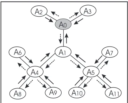
3.2 Inter-agent message passing in MSBNs. . . 38

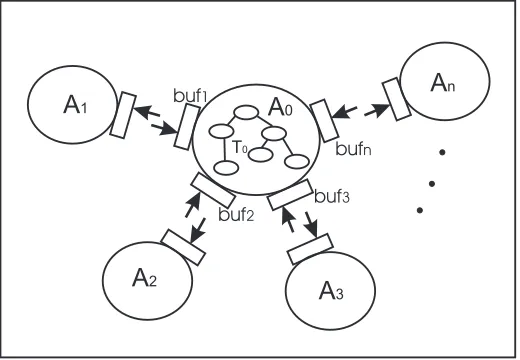
3.3 Incoming message buffers. The agentA0maintainsnmessage buffers each responding to an adjacent agent. . . 41

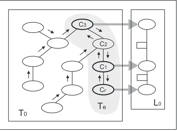
3.4 An example of partial propagation for calculating a single outgoing mes-sage. Shown with the local JT T0, linkage tree L0 and extended linkage host treeTe. . . 44

3.5 An example of partial propagation for updating local calculating a single outgoing message. Shown with the local JT T0, linkage tree L0 and ex-tended linkage host treeTe. . . 49

4.1 (a) The JT constructed from the BN in Figure 2.1. (b) Inward message passing, and (c) Outward message passing with clusterdef as the root. . . . 61

4.2 Allocating separate marginals according to the ASM procedure. . . 67

(12)

4.3 (a) A sample BN. (b) The corresponding JT with multiple initialization options. . . 74

5.1 Conceptual view of PM factors in an LJF. . . 84 5.2 Passing of PM messages. (a) A conceptual view, and (b) Actual calculation. 90

6.1 An LJF with (a) the subnets, (b) the hypertree and (c) the LJF with linkage trees and local JTs. . . 104 6.2 Estimation of extended linkage potentials for non-root linkages. . . 109 6.3 Examples of extended linkage potentials calculation. . . 110 6.4 Performance of LLAIS, compared with two variations of LJF local

impor-tance samplers: MSE for each of 30 test cases plotted against the probabil-ity of evidence. . . 113 6.5 Convergence of extended linkage potentials of 4 linkages simulated in a test run

of LLAIS. . . 114

7.1 BK approximation in a small DBN with a forward interface as{a1, c1, d1} . 122

7.2 A sample MA-DBN.(a) The organization graph, and (b) the local transition graphs. . . 127 7.3 An MA-DBN compiled into an LDJF. (a) the MA-DBN (b) LDJF1 (c)

LDJFT . . . 129

7.4 MA-DBN re-factorization. . . 136

(13)

Chapter 1 Introduction

An intelligent agent is usually defined as a computational or natural system that senses its environment and takes actions intelligently according to its own goals [92]. Such an agent can process local observations, generate appropriate decisions and execute the chosen ac-tion. Some examples include autonomous mobile robots, internet infobots and intelligent tutors. Aprobabilistic agentuses probabilistic knowledge representations and reasons ex-plicitly with regard to the state of the domain. For instance, the driverless car, which won the DRAPA Grant Challenge in 2005, has demonstrated the power of a real world proba-bilistic application on a single-agent mobile robot.

In recent years, systems involving multiple agents that communicate with each other in a distributed fashion have become more prevalent. Cooperative agents need to reason collectively about the states of an uncertain domain based on their local knowledge and inter-agent communication. This can happen either in a static time-invariant or a dynamic temporal environment. For instance, one problem is how four driverless cars on a city street can collaborate with each other and coordinate their actions, in order to avoid any collision and safely pass a four-way-stop intersection. We are facing the challenge of how to fully utilize and extend the existing representation models and inference algorithms for a single probabilistic agent to multi-agent settings.

One well-studied model for cooperative multi-agent probabilistic reasoning is the Mul-tiply Sectioned Bayesian Network(MSBN) extended from the traditional Bayesian network (BN) model. With an MSBN, we can decompose a larger problem domain into subdomains,

(14)

CHAPTER 1. INTRODUCTION 2

each individually represented and managed by a relatively lightweight single agent. Multi-ple agents can collectively reason about the state of the global domain based on their local knowledge, local observation, and limited inter-agent communication. Existing inference calculation in MSBN is carried out in some secondary structures, typically alinked junc-tion tree forest(LJF). An LJF consists of local junction trees (JT) each for an agent’s local domain and linkage trees connecting a pair of neighboring agents.

In this thesis, we show that while an LJF provides a coherent framework for exact in-ference with MSBNs, it is too costly to carry out efficient computation with the current Hugin-based message passings. We introduce techniques extending the BN Shenoy-Shafer architecture to the LJF inference structure for improved efficiency of exact global propa-gation. Not only is our method able to avoid the repeated local updates, but it also avoids full rounds of local message passing completely. Still, in larger and more complex prob-lem domains, the exponential computation of LJF global inference could render any exact representation and calculation mostly impractical. It is thus natural to consider the possi-bility of trading off exact inference against the calculation speed and communication cost with approximate approaches. Unfortunately, although approximate techniques have been well-developed in traditional BNs, their extension to MSBNs has been very limited. In the second part of this thesis, we thus focus on the design of alternative approximate solutions to the existing MSBN based multi-agent probabilistic inference. Last but not the least, we move on to the dynamic problem domain and present a novel model that describes the tem-poral evolvement of dynamic agents. Our new model supports effective online monitoring for a group of cooperative agents with bounded errors.

Overall, we propose solutions to the following three questions in this thesis:

1. How to improve the efficiency and robustness of existing exact inference algorithms;

2. How to apply practical approximation techniques in an MSBN model;

3. How to effectively model and reason with a group of dynamic probabilistic agents.

(15)

1.1 Improving Message Passing in LJFs

Most existing inference algorithms are applied on an LJF with Hugin-based recursive mes-sage scheduling schema for inter-agent communication. This results in excessive amount of local computation because each agent’s local belief has to be updated repeatedly, and each update triggers a round of message propagation in the agent’s LJF local JT. Extending from the BN Shenoy-Shafer message passing, we propose a new message oriented archi-tecture for LJFs, such that all inter-agent messages are explicitly calculated and buffered. We will show that although the total number of external messages remains the same, it is much more efficient to compute these messages with our new architecture. This improve-ment is due to that repeated local updates are no longer needed, and local message passings are conducted more efficiently through a partial propagation. We completely avoid any full round passings of local messages.

With the traditional recursive methods, inter-agent message passing is very sensitive to unreliable communication channels. Also, periodical off-line times can prevent each agent from observing local evidence continuously. We thus try to support the exact MSBN belief updating with iterative message passing. We present an iterative version of our new ar-chitecture, along with a scheme that avoids repeated multiplications during message com-putation. We show that the convergence of iterative message passing to exact results is guaranteed. More importantly, temporary communication errors can be tolerated without causing global belief updating failures.

1.2 Marginal Calibration

(16)

A fast calibration ensures efficient global inference. With all existing algorithms, the marginal calibration is carried out through standard inter-agent messages passings. Such a calibration process is implicit and is usually expensive in both time and space. In this thesis, we introduce a marginal calibration algorithm based on the theories developed for the cluster calibration in traditional BN junction trees and our new LJF message passing architecture.

The global propagation (GP) method used in the Hugin architecture is arguably one of the best methods for exact probabilistic inference method in BNs. Passing messages between clusters (cliques) in a JT is the basic operation in the GP method. It is traditionally considered that the messages passed are simply potentials without any specific semantic meaning. We study the factorizations of a joint probability distribution defined by a BN before and after the GP method is performed, and we investigate the messages passed algebraically. We reveal that the messages are actually separator marginals or their factor-izations, thus passing messages in the GP method can be equivalently considered as the problem of allocating separator marginals. This novel perspective of propagation gives rise to a more efficient way of computing cluster marginals with both the Hugin and the Shenoy-Shafer message passings.

Extending the above results, we design an MSBN marginal calibration algorithm that requires the minimum inter-agent message passing and local computation. We introduce the concept of prior marginal (PM) factors for a complete prior distribution of MSBN subnets. Based on a distributed analysis of these factors at the compile time, we can guide the actual runtime inter-agent communication by sending only the necessary messages.

1.3 Localized Stochastic Sampling in MSBNs

(17)

explore only a small part of the entire multi-agent domain space.

We thus aim to maintain the LJF framework and explore localized approximation, which is realized through an individually carried out sampling process at an agent’s subnet. In a calibrated local JT, such local approximation is possible, but standard BN sampling algorithms can not be applied directly. One major obstacle is the need for supporting the agent message calculation over linkage trees. We should be able to obtain an inter-agent message, which is composed of a set of extended linkage potentials, accurately and efficiently with the local sampling algorithm.

As we study the extension of BN importance sampling techniques to JTs, we present a novel LJF-based Local Adaptive Importance Sampler (LLAIS). We design our importance function as tables of posterior probabilities over the clusters of an LJF local JT. We adopt the adaptive importance sampling, such that the importance functions are learned sequen-tially to approach the optimal sampling distribution. One innovative feature of the LLAIS is that it facilitates inter-agent message calculation. We can obtain an approximation of a linkage tree message from the learned importance function before the local sampling is completed.

1.4 Multi-agent Probabilistic Reasoning in Dynamic

Do-mains

Another problem investigated in this thesis is the representation models and inference al-gorithms for a dynamically evolving multi-agent system. Cooperative agents often need to reason about the states of a domain that changes over time. For example, in many appli-cations, agents need to track the state of such systems, a problem known as tracking, or monitoring. Essentially, each agent needs to determine the posterior probability for nodes of interest, given a set of accumulated evidence from the agent’s own observation and those of other agents. Online monitoringrequires the calculation of monitoring results at each time step at runtime.

(18)

multi-agent probabilistic reasoning, it is restricted to static problem domains. On the other hand, the dynamic Bayesian network (DBN) model is well known for modeling dynamic (temporal) domains involving a single agent. We are thus motivated to search for a possible combination of the two for representing dynamic uncertainty knowledge in a multi-agent setting. However, several obstacles to such integration exist. In particular, a decomposed representation of joint JPD does not guarantee efficient inference calculation in dynamic domains. The spatial distribution of the multi-agent systems could conflict with the tempo-ral message passing for dynamic multi-agent probabilistic reasoning.

Our solution to a compact representation and effective inference framework is to ex-ploit weak interactions between each dynamic agent’s individual evolvement over time. By assuming certain level of independency among the temporal advance of the cooperative agents, we can take the advantage of both MSBN and DBN models and provide an ap-proximate solution to the multi-agent online monitoring problem with a new model named as Multi-Agent Dynamic Bayesian Networks (MA-DBN). While agents are organized ac-cording to an underlying hypertree structure to facilitate inter-agent communication, each dynamic agent maintains an individual chain of evolution. We introduce a new secondary structure of an MA-DBN called LDJF, which enables a factorized and more efficient com-putation of the cooperative online monitoring.

1.5 Thesis Overview

The organization of the thesis is summarized below:

(19)

• Chapter 3: An Improved LJF Message Passing ArchitectureIn this chapter, we present a new message passing architecture for MSBN LJFs. Different from the tra-ditional Hugin-based message passing, our new approach adopts from the Shenoy-Shafer architecture by utilizing linkage trees as message buffers. An inter-agent mes-sage can be originated from either a consistent or inconsistent local JT, and a full local update is never issued. The new architecture can be extended to allow asynchronized passing of iterative messages; such a scheme maintains the correctness of the exact message calculation with improved robustness of inter-agent communication.

• Chapter 4: BN Prior Marginal FactorsIn this chapter, we examine the problem of JPD factorization in traditional single-agent BNs. We investigate the semantic mean-ing of messages passed over the separator of each pair of neighbourmean-ing JT clusters. We present a procedure named Allocate Separator Marginal(ASM) to determine the actual information a cluster requires to form the marginal in the JT. We show how the ASM procedure can help to form the marginal with a minimum messages passing.

• Chapter 5: Fast Marginal CalibrationCurrent MSBN calibration methods are per-formed implicitly and expensively in terms of both inter-agent messages passing and local computation. They are not suitable when an explicit prior marginal is needed for certain subnets. In this chapter, we present a new marginal calibration algorithm that is based upon informed message passing; not only does it provide a correct prior explicitly, but it also requires a minimum amount of inter-agent messages and local calculation.

(20)

messages.

• Chapter 7: MA-DBN: Modeling Agents’ Dynamic Evolvement In this chapter we turn to dynamic problem domains. We present a dynamic model, MA-DBN, that supports distributed multi-agent probabilistic inference. We model the dynamics of a group of cooperative agents approximately by utilizing weak interactions among them. We show that the error resulting from such assumption of independency is bounded over time during the course of online monitoring. We also introduce a method of re-factorization to reduce the correlation between two adjacent dynamic agents.

(21)

Chapter 2 Background

This chapter presents a brief introduction to probabilistic graphical models, particularly, the Bayesian network model and the multiply sectioned Bayesian network model. We discuss major exact and approximate inference algorithms for BNs. We also introduce the secondary structure of MSBNs, a linked junction tree forest, as well as its existing inference algorithms.

2.1 Probabilistic Graphical Models

Probabilistic graphical models have become an important tool in helping an intelligent agent to reason with its uncertainty knowledge and to take proper actions. They utilize graphs to compactly represent a complex probabilistic distribution, such that data are mod-eled as a set of nodes representing random variables, and their connecting arcs, directed or undirected, encode the dependencies between the variables. Probabilistic graphical models combine the representation and algorithmic powers of both the probability theory and the graph theory. We will present a brief introduction that is pertinent to our work in later chapters. A more comprehensive introduction can be found in [41] [45].

(22)

CHAPTER 2. BACKGROUND 10

2.1.1 Basic Probability Theory

Based on probability theory, arandom variableis a variable whose outcomes (values) are given by chance. The possible outcomes of a discrete random variable are mutually exclu-sive and collectively exhaustive, and together as a set, called the domain of the variable. The probability of a random variable is measured by a function that maps each possible outcome, orinstantiation, of this variable into the interval of [0,1].

In this thesis, we restrict our discussion to multiple-valued discrete random variables. Capital letters or indexed capital letter, such asA, B, orXi denote random variables,

un-less otherwise specified. Bold capital letters, such as X, or Y, denote sets of variables. Bold capital letter E is usually used to denote the set of evidence variables. Lower case letters, such as a and x denote particular instantiation of variable A and X respectively, unless specified otherwise. Bold lower case letters, such asxand y, denote particular in-stantiations of sets X and Y respectively. Bold lower case letter e is used to denote the observation for the set of evidence variablesE.

Given a set of random variables V = {V1, V2, ..., Vn}, the probabilities of all

com-binations of the possible outcomes of each variable in V is called the joint probability distribution(JPD) ofV, which is denoted as

P(V) =P(V1 =v1, V2 =v2, ..., Vn =vn) = P(v1, v2, ..., vn),

wherev1, v2, ..., vnare the respective values those variables take. ThedomainofV is the

cross join of the domains of all variables in{V1, V2, ..., Vn}. Each element from the domain

of a set of variables is referred to as an instantiation of these variables.

The probability distribution of a subset X of V can be obtained by summing out all variables in set ofVexcludingX(denoted byV\X):

P(X) = X

V\X

P(V),

whereP(X)is called themarginal probability distribution(MPD) ofXfromP(V). It can also be written asP↓x₍_V₎_{. In general, the process of summing out some variables from a}

(23)

Given that we have some random variables observed with certain values, the probability distribution of other random variables may change. This relationship of dependency is expressed by a conditional probability distribution (CPD). Let X and Y be two disjoint subsets of V and x and y be their instantiations. The CPD of X = x given Y = y, denoted byP(X=x|Y=y)and abbreviated asP(x|y), is defined as

P(x|y) = P(x,y)

P(y) . (2.1)

whereP(y)6= 0.

Equation 2.1 defines the probability ofX=xgivenY =y, where Xis theheadand

Yis thetailof this CPD.

The conditional probability distribution of some variables X with given evidence e , denoted as P(X|E=e), is also known as theposterior probability distribution ofX. In this thesis, we will consider onlyhard evidencesuch that each evidence is an instantiation of a variable. The marginal probability distribution can be viewed as a special case of conditional probability distribution when evidence is not yet observed for any variables. Thus, it is also referred to as theprior marginal distributionor just thepriorin this thesis.

2.1.2 Dependency Model

A complete specification of JPD defines a probabilistic model for a set of random variables. However, to specify a probability model using a full JPD table is impractical. For a domain described bynboolean variables, it requires a table of sizeO(2n₎_{and takes}_O₍₂n₎_{time to}

process the table. By taking advantage of the dependence and independence relationship among variables, this cost can be reduced greatly.

LetX,Y andZbe disjoint subsets ofV. XandY areunconditionally independentif the following holds:

(24)

XandYareconditionally independentgivenZif the following holds:

P(X|Y,Z) = P(X|Z), P(Z)6= 0. (2.3) The conditional independency relationship in Equation 2.3 can be denoted as a condi-tional independency statement(CIS) I(X,Z,Y) orI(X,Y|Z). The unconditional inde-pendency relationship in Equation 2.2 can be denoted as CISI(X,∅,Y)orI(X,Y|∅). A dependency model is any modelM of a set of variablesV = {V1, V2, ..., Vn}from which

one can decide whetherI(X,Y|Z)is true or not for all possible disjoint subsetsX,Yand

Z.

An easy and intuitive approach to model some dependency models is the use of directed acyclic graphs (DAG). A DAG consists of a set of nodes as the random variables, and a set of directed links between nodes but with no directed cycles. The independency relationship in a DAG can be identified by a graphical criteria calledd-separation.

Definition 1 D-separation

VariablesXandY in a DAG are d-separated if for all paths connectingXandY, there is an intermediate variableZ such that one of the following statement is satisfied.

1. Zis the middle variable in one or a serial of diverging connections, andZ is instan-tiated as an evidence.

2. Z is the middle variable in a converging connection, and neither Z nor any of its descendants have been instantiated.

IfZd-separatesXandYin the graphG, then the CISI(X,Z,Y)is said to be derived from G. A causal network is a directed graph constructed based on a special list of CIS calledcausal input list, where the random variables are ordered such that a cause always precedes its effect.

2.2 Bayesian Networks

(25)

systems that must function with uncertain knowledge, such as machine learning, speech recognition, bioinformatics, error-control codes, medical diagnosis and so on.

Denoted as a tripletB = (V,D, P), a BN consists of a set of random variablesV, a DAG D where each variable inV corresponds one to one to a node in D. Each variable

Vi inV is represented as a node in the DAG and is associated with a CPDP(Vi|P a(Vi)),

whereP a(Vi)denotes the parents ofVi in the DAG. The product of these CPDs defines a

JPD as:

P(V) = Y

Vi∈V

P(Vi|P a(Vi)), (2.4)

and we call this factorization (in terms of CPDs) aBayesian factorization. The BN model captures the independency among random variables and provides a compact representation of JPD. Alternatively and equivalently, a BN can be defined in terms of the CPD factoriza-tion of a JPD.

Definition 2 LetV ={V1, . . . , Vn}. Consider the CPD factorization ofP(V)as below:

P(V) = Y

Vi∈V, Vi6∈Ai,Ai⊆V

P(Vi|Ai), (2.5)

If (1) each Vi ∈ V appears exactly once as the head of one CPD in the above

factoriza-tion, and (2) the graph obtained by depicting a directed edge from vertexXtoVi for each

X ∈Aiis a DAG,i= 1, . . . , n, then the obtained DAG and the CPDsP(Vi|Ai)in

Equa-tion (2.5) define a BN. In fact, the factorizaEqua-tion in EquaEqua-tion 2.5 is a Bayesian factorizaEqua-tion of the defined BN.

The graphical structure of DAG encodes CIs that are satisfied by the JPD defined by the Bayesian factorization. In particular, the Markov independence statement states that every vertexViin a DAGDis independent of its non-descendants (denotedNonDesc(Vi))

given its parentsP a(Vi), i.e.,I(Vi, P a(Vi), N onDesc(Vi)). We will useMarkov(D)to

(26)

g h

f

e c

b a

d

p(h|f)

p(g|h) p(d|b) _p(e|b) p(a)

p(f|cd) p(c|a)

p(b)

Figure 2.1: A simple BN: the Asia travel network.

Consider the Asia travel BN [52] defined over V = {a, . . . , h}. Its DAG and the CPDs associated with each node are shown in Figure 2.1. The JPDP(V)is obtained as:

P(V) = P(a)·P(b)·P(c|a)·P(d|b)·P(e|b)·P(f|cd)·P(g|ef)·P(h|f). The DAG encodes CI information, for instance, given b, d and e are independent, i.e., I(d, b, e); givenf,handabcdegare independent, i.e.,I(h, f, abcdeg).

2.2.1 Exact Inference with Junction Trees

A Bayesian network provides not only a natural and compact way to model causal struc-tures, but also a computational basis for probabilistic inference [81]. The most common inference task performed on BNs is the calculation of posterior distributionP(X|E=e)

for a set of variables Xgiven evidence set E. We call the set of variables H = V\X\E

(27)

P(X|E=e) = P(X,e)

P(e) =αP(X,e) = α

X

H

P(X,e,H), (2.6) whereαis a normalization value1/P(e).

The above inference calculates the result exactly according to the probability theory. This is known as exact inference calculation. However, such brute force calculation is computationally infeasible. In fact, many algorithms have been developed that are based on the same notion of a BN, but with considerably different underlying concepts. A group of exact algorithms perform the task of probabilistic inference on a secondary structure of a JT. A JT is a tree graph whose nodes are subsets of the domain variables calledclusters, orcliques. The steps of constructing a JT are sketched as follows.

Step 1. Moralizing the original graph: A moral graph is constructed by first connecting every pair of nodes in each node’s parent set if they are not connected; then replacing the directed edges with undirected edges.

Step 2. Triangulating the moralized graph: Add necessary edges so the moral graph is trian-gulated. In a triangulated graph, every cycle of length 4 or more has at least one link between two non-adjacent nodes on the cycle. Different triangulation algo-rithm may have different results. The problem of finding an optimal triangulation is NP-complete [105], but fast algorithms that produce high quality results are avail-able [19] [8].

Step 3. Identifying and joining cliques to construct a JT: Acliqueor just aclusteris a com-plete and maximal subgraph of a triangulated graph. Once the clusters are identified, they are arranged to form a JT. A method to construct an optimal JT is discussed in [37] where the clique intersection with largest state space (the number of configu-rations) is preferred at each construction step.

(28)

Once a JT is constructed, each JT cluster will be quantified with an initial function Φ, known as the potentialof the cluster. 1 _{As each CPD}_P₍_X

i|P a(Xi))is assigned to a JT

cluster containing{Xi} ∪P a(Xi), the initial potential of a cluster is then the product all

CPD the cluster has received. If a cluster does not receive any CPD, it will be initialized to a unity potential 1.

After the JT initialization, the potential of each cluster does not represent the cluster marginal. In order to transform the cluster potential into the cluster marginal, the prob-ability information of each cluster must be updated to be consistent to other clusters. In particular, when evidence is observed, they are entered into some clusters and need to be propagated throughout the JT. The property of running intersection ensures the coherent in-formation exchange among JT clusters through message passings over the separators. The Hugin architecture [40] [59] and the Shenoy-Shafer architecture [82] [83] [84] are the two major variations for the JT-based exact inference calculation.

The Hugin Architecture

Under the Hugin architecture, there is a message buffer for each separator to enforce the consistency between adjacent clusters on common variables. The potential associated with each separator is initialized to unity potential 1, and the Huginglobal propagation(GP) is carried out based on message passings. First, an arbitrary cluster in the JT is chosen as the root cluster and all the edges of the JT are directed toward the root. Then, messages between clusters are calculated and propagated in the cluster tree through two stages, namely, the inward and outward passing stages, also known as the Collect-Evidence stage, and the Distribute-Evidence stage. During the inward pass, each JT cluster passes a message to its neighbor towards the root’s direction, beginning with the cluster farthest from the root. During the outward pass, each cluster in the JT passes a message to its neighbor away from the root’s direction, beginning with the root itself.

(29)

Suppose a message is to be sent from clusterC1 to clusterC2, and the potential

associ-ated with senderC1isΦ(C1). The messageMC1→C2 is calculated as

MC1→C2 = Φ(C1)

↓C1∩C2_, _(2.7)

whereC1∩C2 is the set of nodes in the separator betweenC1andC2.

In Hugin architecture, a message calculated by Equation 2.7 is not directly multiplied to the receiving neighbor, but is divided by the existing potential in the separator and then stored as a new separator potential. This updated potential on the separator is the actual value to be absorbed in the receiving cluster. We illustrate a single message passing under the Hugin architecture in Figure 2.2. Note that passing a Hugin message will result in updated potential values for the receiving cluster as well as the separator.

C2

C1

Mold

Potential = Potential * Mnew/ Mold Mnew

Message direction separator

BEFORE

Potential does not change

AFTER

C1

C2

Figure 2.2: Before and after a single message passing in the Hugin architecture.

Once the GP is completed, the JPD of all variables is equal to the product of potentials on all clusters divided by the product of potentials on all separators. Meanwhile, the po-tential of each cluster and separator has transformed into marginal. The marginal of some variable of interestXcan be calculated by first locating a clusterC that containsX. Then, we marginalize the cluster potentialΦ(C)onXto obtain

(30)

whereeis the evidence incorporated before applying the GP method. GivenP(X,e)and

P(e), The posterior distribution can then be calculated following Equation 2.6.

The message passing on the Hugin architecture can be improved by the method of Lazy inference [57] [58] [56]. Instead of maintaining a single potential for each cluster and sep-arator in the Hugin architecture, we keep a multiplicative decomposition of potential tables for the clusters and separators in the Lazy inference. We can thus delay the actual com-bination of potential tables during the multiplication calculation, so we are able to exploit independence relations introduced by evidence during the message calculation.

The Shenoy-Shafer Architecture

In the Shenoy-Shafer architecture, the global propagation is also executed as message exchanges over the separators, but each separator is associated with two message buffers for storing messages passed in each direction between the two clusters.

With the Shenoy-Shafer message passing scheme, each cluster waits to send its mes-sage to a given neighbor until it has received mesmes-sages from allotherneighbors. Unlike the typical rooted recursive scheduling for Hugin message passings, no root cluster is selected in the Shenoy-Shafer architecture. When a cluster is ready to send its message to a particu-lar neighbor, it computes the message by collecting all the buffered messages from its other neighbors, multiplying its own table by these messages and marginalizing the product over the separator between itself and the neighbor to whom it is sending [84].

Figure 2.3 shows the calculation of a Shenoy-Shafer message. Suppose we have a JT clusterC andNC is the set of its neighboring clusters. The messageC has received from

any neighboring cluster N is denoted as MN→C, then the message C sent to a specific

neighborC0 _{is given by}

MC→C0 = (Φ(C)·

Y

N∈NC\C0

MN→C)↓C∩C

0

. (2.9)

(31)

C C

’

Message from C to C’

Message from C’ to C

Nc

\ ’

C

two message buffers

Figure 2.3: Message passing in the Shenoy-Shafer architecture.

clusters do not change during a single Shenoy-Shafer message passing.

The global propagation is completed when all clusters have sent and received messages from all their neighbors, or equivalently, when each message buffer is filled with a message. The marginal on a clusterC, with evidencee incorporated before the propagation, can be calculated as

P(C,e) = P(V)↓C _{= Φ(}_C₎ Y N∈NC

MN→C. (2.10)

The original potential table and all the messages it receives from all its neighbors are multiplied together to obtain the cluster marginal. The marginal of some certain variables can be calculated by marginalizing the JT cluster that contains the variables, followed by normalization as described in Equations 2.8 and 2.6.

(32)

neighboring clusters, under either the Hugin or the Shenoy-Shafer architecture, contains essentially the same information. The difference lies in the message calculation schema adopted by the two architectures: the explicit form of messages which a cluster receives does not appear in the Hugin architecture, whereas each message is individually stored in the Shenoy-Shafer architecture.

According to the comparison conducted by Lepar [53], the overall computational effi-ciency between the Shenoy-Shafer and the Hugin architectures depends on the structure of the original BNs. The Hugin architecture is faster on arbitrary JTs. However, the Shenoy-Shafer architecture answers queries for a wider variety of applications, and it delivers better performance in a special tree structure, binary join trees, in which each cluster has at most three neighbors [67].

Exact inference in BN is NP-hard in the worse case [16]. JT algorithms, including both the Hugin and the Shenoy-Shafer architectures, do not solve the problem of NP-hardness as well. Exponential time and space are required when these algorithms are applied to JTs that are constructed from densely connected networks. The network density is usually captured by a graph parameter calledtree-width, which represents the size of the largest JT cluster.

2.2.2 Approximation Methods

In larger BNs, exact inference, including the JT algorithms, become impractical. An al-ternative is to use approximate inference to obtain a result that is close to exact. Although approximation with guaranteed error bounds is also NP-hard in worse cases [18], the class of solvable problems is wider and some approximation strategies work well in practice. Two approximation methods pertinent to this thesis are briefly introduced as follows.

Stochastic Sampling

(33)

of the inference task. The accuracy depends on the size of samples; the execution time is linear in the sample size and is mostly independent of the network topology. Stochastic algorithms have a nice any-time property such that the computation can be interrupted at any given time to yield an approximation. [33].

Probabilistic logic sampling is the first and simplest sampling algorithm [34]. Samples are obtained in a BN following the directed edges from the root; any samples that are inconsistent with the observed evidence values (if any) are discarded. The probabilities of query nodes are obtained by counting the frequencies with which relevant events occur in the sample set. Logic sampling works very well in the absence of evidence. But with evidence, the number of accepted samples decreases exponentially with the number of evidence variables, resulting in a large amount of wasted samples.

The algorithms of likelihood weighting or evidence weighting [80] [29] solve the prob-lem of sample waste in logic sampling. In likelihood weighting, when an evidence node is encountered in the sampling process, the observed value of the evidence node is recorded, and the sample is weighed by the likelihood of evidence conditional on the samples. Like-lihood weighting algorithm can be applied in larger networks and converges faster then logic sampling. However, the main difficulty with likelihood weighting, and indeed with most stochastic sampling algorithms, is that it takes a long time to converge for unlikely events [33] [15].

Importance sampling algorithms improve these sampling approaches by using a revised sampling distribution to approximate the posterior distributions. Such a sampling distribu-tion can be generated in many ways. A successful method is the Adaptive Importance Sampling for Bayesian networks (AIS-BN) [15], which reduces the sampling variance by learning a sampling distribution that is as close as possible to the optimal importance sam-pling function.

(34)

Structure Simplification

These methods approximate the inference calculation by applying a certain level of simplification to the original model. These algorithms try to weaken or ignore some of the networks dependencies, forcing the generated dependencies of the network to result in a bounded error during the inference calculation. Such a simplification could involve reduc-ing the cardinality of the size of JT clusters [48], or fittreduc-ing parameters to a simple logistic function [62]. Another widely applied method is to reduce edges of an original network. For example, the edges representing weak dependencies can be removed to simplify the inference calculation [43].

2.3 Multi-agent Probabilistic Reasoning with MSBNs

In a multi-agent setting, the problem domain is naturally distributed among agents, and typically with increased size and complexity. Modeling such a domain as a single BN and performing inference tasks have been known to be difficult [92]. It is thus natural to consider decomposing one single large and complex domain into subdomains, which can be individually represented and managed by a relatively lightweight single agent. We assume that agents are cooperative such that they provide only truthful information about their local domains to other agents.

Multiply Sectioned Bayesian Network(MSBN) [92] [100] extends the traditional BN model from single-agent oriented paradigm to distributed multi-agent paradigm. The MSBN model is introduced based on following five basic assumptions that describe some ideal knowledge representation formalisms for multi-agent uncertain reasoning [99] [101].

1. Agent’s belief is represented as probability.

2. Agents communicate their beliefs based on a small set of shared variables.

3. A simpler agent organization is preferred.

(35)

5. An agent’s local JPD admits the agent’s belief of its local variables and the shared variables with other agents.

It has been shown that based on this small set of requirements, the resultant representa-tion of a cooperative multi-agent system is an MSBN [101]. Formally, an MSBN is defined as the followings [92].

Definition 3 Let G = (V,E) be a connected graph, with the set of random variables V

and connecting edgesE, sectioned into subgraphs{Gi = (Vi, Ei)}. Let the subgraphs be organized into an undirected treeHwhere each node is uniquely labeled by aGiand each link betweenGkandGmis labeled by the non-empty interfaceVk∩Vmsuch that for each i and j,Vi∩Vj is contained in each subgraph on the path betweenGiandGj inH. Then His a hypertree over G. EachGi is a hypernode and each interface is a hyperlink.

Definition 4 Let G be a directed graph such that a hypertree over G exists. A node x contained in more than one subgraph with its parents P a(x)in G is a d-sepnode if there exists at least one subgraph that containsP a(x). An interface I is a d-sepset if everyx∈I

is a d-sepnode.

Definition 5 A hypertree MSDAGG=∪iGi, where eachGiis a DAG, is a connected DAG such that (1) there exists a hypertreeHover G, and (2) each hyperlink inHis a d-sepset.

Definition 6 An MSBN M is a triplet (V, G, P).V=∪iVi is the domain where eachViis a set of variables. G=∪iGi (a hypertree MSDAG) is the structure in which nodes of each DAGGi are labled by elements ofVi. Let xbe a variable and P a(x)be all the parents ofxin G. For eachx, exactly one of its occurrences (in aGi containing{x} ∪P a(x)) is assignedP(x|P a(x)), and each occurrence in other DAGs is assigned a uniform potential. P =Q_iPiis the JPD, where eachPiis the product of the potentials associated with nodes inGi. A tripletNi = (Vi, Gi, Pi)is called a subnet of M. Two subnetsNiandNj are said to be adjacent ifGi andGj are adjacent on the hypertree MSDAG.

(36)

a tree structure. Each hypertree node corresponds to a subnet, and each hypertree link cor-responds to a d-sepset, which is the set of shared variables between adjacent subnets. A hyperlink renders two sides of the network conditionally independent similar to a separator in a JT. A hypertreeH is purposely structured so that (1) for any variablex contained in more than one subnet with its parents P a(x) in G, there must exist a subnet containing

P a(x); (2) the shared variables between any two subnetsNi andNj are contained in each

subnet on the path betweenNiandNj inH.

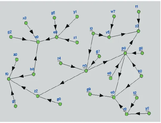
One small example of MSBN for digital equipment monitoring, borrowed from Xiang’s paper [94], is shown in Figure 2.4. The digital equipment consists of 5 individual physical components. Each component contains the logical gates along with the labels for its input and output signals as shown enclosed in a box in Figure 2.4 (a). A set of 5 agents, each maintaining one component, cooperate to monitor the equipment and trouble-shoot. The hypertree of the constructed MSBN is shown in Figure 2.4 (b). Each agent is responsible for its own subdomain knowledge regarding the gates of the component and local obser-vation. For example, Figure 2.5 shows a subnet maintained by one agent. Agents share information over the gates that connects two components. Thus, through limited local ob-servation and communication, agents can cooperate to determine the current functioning status of the equipment, and identify faulty gates when mal-functioning occurs [96].

MSBNs provide a framework for uncertainty reasoning in cooperative multi-agent sys-tems, so that a distributed problem domain can be modeled modularly and the inference to be performed coherently. MSBNs have been successfully applied in areas such as building surveillance [31], medical and equipment diagnosis [103] [96], distributed collaborative design [95] and multi-agent ambiguous context clarification in pervasive environments [3]. MSBNs also provide support for object-oriented Bayesian networks [47].

2.3.1 Linked Junction Tree Forests (LJFs)

(37)

G

1

G

3

G

4

G

2

G

0

(a)

(b)

(a)

Figure 2.4: An example of digital equipment monitoring system. (a) The equipment, (b)The hypertree of corresponding MSBN.

A linkage tree is just a special name for the JT constructed from a d-sepset. In a linkage tree, each cluster is called alinkage, and each separator, alinkage separator. The cluster in a local JT that contains a linkage is called alinkage host. Two adjacent subnets will each maintain its own linkage tree that corresponds to the same d-sepset. These two linkage trees may be different, but only at their topologies. As they span over the same d-sepset and have an identical set of clusters and separators, it has been proven that the result of message passing is not affected [92].

(38)

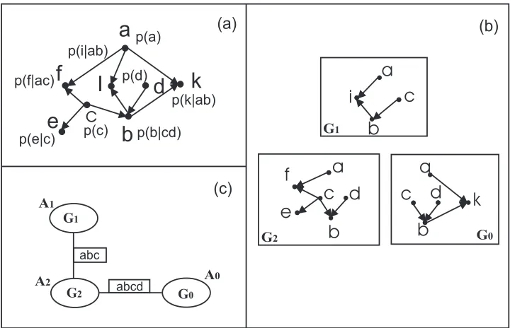
Figure 2.5: One subnet of the MSBN in Figure 2.4.

with the hypertree Figure 2.6 (c), comprise an MSBN. Two hyperlinks in Figure 2.6 (c) consist of the d-sepsets{a, b, c}and{a, b, c, d}. The subnets are maintained by agentsA0,

A1 andA2 respectively. Note that the union of the three DAGs in Figure 2.6 (b) gives rise

to the DAG in Figure 2.6 (a).

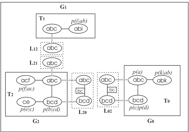
Figure 2.7 shows an LJF constructed from the MSBN in Figure 2.6 (b) and Figure 2.6 (c). Local JTs,T0,T1 andT2 constructed from BN subnetG0,G1 andG2 respectively, are

enclosed by boxes with solid edges. Linkage trees, converted from d-sepsets, are enclosed by boxes with dotted edges. Note that each pair of adjacent subnets maintain the identical linkage trees in this example. The linkage treeL02 contains two linkagesabcandbcdand

their linkage hosts inT0are the clusters{abc}and{bcd}.

(39)

abcd abc

p(f|ac)

p(a)

p(k|ab)

p(b|cd) p(i|ab)

p(d)

p(c) p(e|c)

e

b

k

d

I

f

a

(a)

(c)

(b)

Figure 2.6: (a) A BN. (b) A small MSBN with three subnets. (c) The corresponding MSBN hypertree.

clusterbcdofG2, is assigned the CPDP(b|cd). All other occurrences are assigned a unity

potential (not shown in the figure). In most cases, the initial potential does not provide the complete information for an agent to correctly reason about its own problem subdomain. This is because the local JTs are not yet consistent, but more importantly, the potential of each subnet does not represent the prior marginal distribution, which is the JPD of the local variables without any observed evidence.

For example, the initial potentials of all three subnets in Figure 2.7 are: Φ(G0) =

(40)

Figure 2.7: An LJF constructed for the MSBN in Figure 2.6.

2.3.2 MSBN Distributed Inference

A major task of MSBN inference is to supply the correct global posterior probabilistic knowledge to each agent given some locally observed evidence. The most dominant group of algorithms for distributed probabilistic inference in an MSBN utilize secondary infer-ence structures [92, 93, 98]. Among them, the LJF-based algorithms, extending from JT-based inference methods for single-agent BNs, have proven to be the most successful [92]. LJF-based inference algorithms are superior to methods based on global loop-cutset con-ditioning and global stochastic sampling [93], as they provide a higher level of autonomy than those alternatives.

However, the existing LJF-based algorithms are based mostly on the extension from Hugin message passings. The typical propagation process requires two rounds of global messages exchange in the corresponding LJF. This can be viewed at a high level as the Hugin message propagation in the context of an MSBN.

Within an LJF framework, inter-agent messages passed between two adjacent agents are calculated over their connecting linkage tree.2 _{During LJF global propagation, inter-agent}

(41)

messages are passed recursively inward and outward, relative to a randomly selected root subnet. During the inward message passing, each agent passes a message to its neighbor toward the root’s direction, starting with the leaf subnets. During the outward passing, each agent passes a message to its neighbor away from the root’s direction, originating from the root itself.

With the existing Hugin-based methods, an agent’s local computation is costly. The consistency of the local JT must be achieved in the sender before passing an inter-agent message, and also in the receiver afterward. This local consistency is obtained through the standard JT message passing in the LJF local JT. The number of such local updates in an MSBN subnet is not relative to the root selection during the LJF global propagation, but depends on the hypertree topology. In fact, the existing Hugin-based methods all require repeatedupdates of the local beliefs. Whenever an agent receives an inter-agent message, a full round of message passing in its local JT must be performed, which includes two complete stages of message passings (inward and outward) among the local JT clusters,

2.4 Discussion

A BN, as an example of graphical probabilistic model, has been well accepted as a powerful tool for uncertainty reasoning. Although exact inference as well as approximate inference with guaranteed precision are NP-hard, there have been many practical algorithms that can solve a wide range of inference tasks.

(42)

(43)

Chapter 3 An Improved LJF Message Passing

Architecture

The existing LJF inference algorithms are extensions to the Hugin-based message passing architecture. They are similarly composed of rooted, recursive message passing schema at both the global and the local levels [92]. The global inference is first called upon a randomly selected agent, and two rounds of inter-agent messages passing are recursively carried out among all agents in a restricted order. A message passed between two adjacent agents, known also as an external message or a global message, is transmitted over the linkage trees between the agents. The update of local belief during the local propagation involves passing of intra-agent messages, each known as an internal message or a local messagein the LJF local JT1_.

The original Hugin architecture supports the inference computation in a BN JT with exact results, but its extended version in MSBN LJFs could incur an extensive amount of internal messages passing. This is because each Hugin message is no longer passed be-tween two JT clusters, but instead bebe-tween two MSBN subnets each with its own internal structure of a local JT. Upon receiving an incoming inter-agent message, an agent must absorb it immediately, followed by an update of its local belief that involves two rounds of intra-agent message passings. Also, with the Hugin-based propagation, it is well-known

1_{Hereinafter, we use inter-agent, external and global message, intra-agent, internal and local message}

interchangeably

(44)

CHAPTER 3. AN IMPROVED LJF MESSAGE PASSING ARCHITECTURE 32

that periodical off-line time prevents each agent from observing local evidence continu-ously [88]. The recent improvement of the LJF Hugin-based method extends from the lazy inference algorithm [58]. The calculation of extended linkage potentials is more efficiently carried out with a lazy-based division [98]. Nevertheless, the local computation remains costly, as an agent withsneighbors will still conductstimes local belief updates, each with a complete round of inward and outward local message passings.

Our goal is to improve the local computational efficiency for LJF global propagations. We argue that, as an LJF represents a high level JT, the inference algorithm for LJFs should not be restricted to the extension of a certain class of JT inference algorithms, i.e. the Hugin architecture. In particular, by adopting some new message calculation and passing scheme, we could avoid the repeated local updates.

In this chapter, we introduce an LJF-based inference architecture extending from the Shafer message passing. The main obstacle to such an integration of the Shenoy-Shafer message passing and LJF is the usage of message buffers. Since Shenoy-Shenoy-Shafer messages must always be buffered, an earlier attempt of Shenoy-Shafer extension is applied on a special secondary structure of an MSBN, named double linked junction tree forest (DLJF) [97]. A DLJF provides the needed message buffers, but its construction requires a more sophisticated, message direction dependent compilation process compared to the construction of an LJF. More importantly, extra storage is needed in a DLJF since we need to maintain two sets of JTs (as the term “double” stands for) in order to pass the two messages between each pair of adjacent agents.

(45)

based on a given root, but initiated simultaneously at all nodes. Our asymptotic analysis shows that the time complexity of our new message passing architecture is superior than the current Hugin-based as well as the Lazy extension to LJF inference methods.

Later in this chapter, we introduce an extension of our new global propagation archi-tecture to iterative message passing. Since more than one message are passed toward each direction between a pair of adjacent agents, a temporary missing inter-message will not halt the global propagation. It has been shown that the current Hugin-based message passing architecture cannot be extended successfully to support exact calculation with an iterative scheme [2], whereas our message oriented LJF architecture provides the needed support for such extension.

Under our iterative scheme, each agent performs the local calculation in complete par-allel with other agents. Inter-agent messages are delivered iteratively and as batch. An agent has more autonomy as to decide the time interval for processing received messages and perform local updates. Since the iterative message passing is conducted among agents organized into a hypertree structure, the convergence of inter-agent messages is guaranteed. Meanwhile, each agent’s local belief can be obtained exactly. Such a scheme could be more costly in terms of message calculation, but it is more suitable in a multi-agent environment with unreliable communication channels due to its fault tolerance ability.

3.1 Hugin-based Recursive Inference

3.1.1 Linkage Tree as Separator

In an MSBN, the exchange of the shared information of adjacent agents is through mes-sages passed over their corresponding d-sepset. A linkage tree is an alternative representa-tion of the d-sepset between adjacent agents in an LJF [89]. A linkage tree is constructed with an explicit internal structure, containing clusters (linkages) smaller than the domain of d-sepset in order to reduce the cost of message calculation. A linkage tree, a linkage and a linkage host are defined by Definition 7 [92].

(46)

Initialize L toTi. Repeat the following on a cluster of L until no nodes can be removed: 1. Remove a nodex /∈Iif x is contained in a single cluster C.

2. If C becomes a subset of an adjacent cluster D after step 1., union C into D.

Each cluster l in L is a linkage. Define a cluster inTi that contains l as its linage host and break the tie arbitrarily.

Current LJF inference algorithms [88, 92] are extensions of the Hugin architecture. Inter-agent messages passed between two adjacent agents are calculated over their con-necting linkage trees, which are used as a Hugin separator. For an LJF local JT Ti to

deliver a message toTj overTi’s linkage treeLij, each linkageQi inLij is assigned first a linkage potential, which is

Φ(Qi) = X

Ci\Qi

Φ(Ci), (3.1)

whereCiisQi’s linkage host inTi.

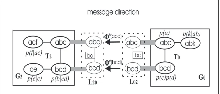
For example, consider the LJF with local JTs and linkage trees shown in Figure 3.1. The message originated from G0 to be delivered to G2 is calculated over the linkage tree

L02, and should consist of the potentials over two linkagesabcandbcd.

(47)

As the linkage tree construction enables a more compact representation of d-sepset, it also introduces redundancy over linkage separators. This is because the separator nodes in the linkage tree may appear more than once in different linkages. For example, consider again the example in Figure 3.1. Using Equation 3.1, we have linkages abcandbcd both carrying information overbc, causing errors in the message propagation.

In order to solve this problem, the concept of extended linkage potential is intro-duced [92]. That is, we first randomly select a linkage as the root linkage and direct all linkages accordingly. Then, we associate each linkage separator with one of its two neigh-boring linkages, which is farther away from the root linkage, as the linkage’s peer separator. The extended linkage potential is defined as follows:

Definition 8 Suppose in a linkage tree, for each linkage Q with peer separator R, the extended linkage potential is defined as follows:

Φ∗(Q) = Φ(Q)/Φ(R) (3.2) for all non-root linkages, and

Φ∗(Q) = Φ(Q) (3.3)

ifQis the root linkage.

Therefore, as the extended linkage potential for root linkage remains the same, the redundancy of the separator information over other linkages is removed by division [92]. For example, in linkage tree L02 from Figure 3.1, we can select the cluster abc as the

root linkage, then associate the separator bc with the linkage bcd as the peer separator. Meanwhile,abchas no peer assigned. The extended linkage potentials on each linkage are

Φ∗₍_abc_{) = Φ(}_abc₎_and_Φ∗₍_bcd_{) = Φ(}_bcd₎_/_Φ(_bc₎_{. The extended linkage potential defined}

in Equation 3.2 is actually used to calculate external messages.

The delivery of an inter-agent message is done through the passing of extended link-age potentials of each linklink-age over the corresponding linklink-age tree. An operation, named

Efficient Probabilistic Inference Algorithms for Cooperative Multiagent Systems

Scholarship at UWindsor

Scholarship at UWindsor

Efficient Probabilistic Inference Algorithms for Cooperative

Efficient Probabilistic Inference Algorithms for Cooperative

Multiagent Systems

Multiagent Systems

EFFICIENT PROBABILISTIC INFERENCE ALGORITHMS FOR

COOPERATIVE MULTI-AGENT SYSTEMS

A DISSERTATION

SUBMITTED TO THE SCHOOL OF COMPUTER SCIENCE

AND THE COMMITTEE ON GRADUATE STUDIES

OF UNIVERSITY OF WINDSOR

IN PARTIAL FULFILLMENT OF THE REQUIREMENTS

FOR THE DEGREE OF

DOCTOR OF PHILOSOPHY

Declaration of Originality

Abstract

Acknowledgement

Contents

List of Tables

List of Figures

Chapter 1

Introduction

1.1 Improving Message Passing in LJFs

1.2 Marginal Calibration

1.3 Localized Stochastic Sampling in MSBNs

1.4 Multi-agent Probabilistic Reasoning in Dynamic

Do-mains

1.5 Thesis Overview

Chapter 2

Background

2.1 Probabilistic Graphical Models

2.1.1 Basic Probability Theory

2.1.2 Dependency Model

2.2 Bayesian Networks

2.2.1 Exact Inference with Junction Trees

’

\ ’

2.2.2 Approximation Methods

2.3 Multi-agent Probabilistic Reasoning with MSBNs

2.3.1 Linked Junction Tree Forests (LJFs)

G

G

G

G

G

(a)

(b)

(a)

e

b

k

d

I

f

a

2.3.2 MSBN Distributed Inference

2.4 Discussion

Chapter 3

An Improved LJF Message Passing

Architecture

3.1 Hugin-based Recursive Inference

3.1.1 Linkage Tree as Separator