Article
Approximate Information and Accelerating for
High-throughput Heterogeneous Data Analysis with
Linear Mixed Models
Shengxin Zhu1,2,†
1 Department of Mathematics, Xi’an Jiaotong-Liverpool University
2 Research Institute of Big Data Analytics, Xi’an Jiaotong-Liverpool University; [email protected];
Tel.: +86-512-8188-4753.
† This paper is based on the presentation FastCalculationofRestrictedMaximumLikelihoodMethodsfor Unbalanced High-throughput Data Analysison 2017 IEEE 2nd International Conference on Big Data Analysis, paper ID (ICBDA2017-289)
Abstract: Linear mixed models are frequently used for analysing heterogeneous data in a
1
broad range of applications. The restricted maximum likelihood method is often preferred to
2
estimate co-variance parameters in such models due to its unbiased estimation of the underlying
3
variance parameters. The restricted log-likelihood function involves log determinants of a
4
complicated co-variance matrix. An efficient statistical estimate of the underlying model parameters
5
and quantifying the accuracy of the estimation requires the first derivatives and the second
6
derivatives of the restricted log-likelihood function, i.e., the observed information. Standard
7
approaches to compute the observed information and its expectation, the Fisher information, is
8
computationally prohibitive for linear mixed models with thousands random and fixed effects.
9
Customized algorithms are of highly demand to keep mixed models analysis scalable for increasing
10
high-throughput heterogeneous data sets. In this paper, we explore how to leverage an averaged
11
information splitting technique and dedicate matrix transform to significantly reduce computations
12
and to accelerate computing. Together with a fill-in reducing multi-frontal sparse direct solver, the
13
averaged information splitting approach improves the performance of the computation process.
14
Keywords: observed information; fisher information; averaged information splitting; approximate
15
information
16
1. Introduction 17
Real-world data like these in animal/plant breeding, clinic trials, ecology and evolution,
18
genome-wide association and many other fields are often heterogeneous. For example, one can
19
not control how many child animals can one animal sire each time. In the clinic trials, individuals
20
in every group are usually not equaled. For many repeated measurements, missing data are very
21
common, which results in heterogeneous data. These cases are different with those in controlled
22
experiments (in a laboratory) where the data usually enjoy a nice controlled block structure. For
23
such controlled structured block data, the classical analysis of variance(ANOVA) approach can give
24
a statistical efficient estimate. On contrast, therestricted maximum likelihood method(REML) introduced
25
in [1] is an attractive method for heterogeneous data analysis. This approach is conceptually
26
simple and is widely used in in animal/plant breeding [2], clinic trials, ecology and evolution
27
[3], genome-wide association [4–7]. And it is receiving increasing attention. In this approach, the
28
underlying observationy∈Rn×1is modeled by the mixed model 29
y=Xτ+Zu+e, (1)
where τ ∈ Rp×1and u ∈ Rb×1 are fixed effects and random effects respectively. e is noise. The
31
random effects and noise are independent normal distribution such thatE(u) = 0, E(e) = 0, u ∼
32
N(0,σ2G),e∼N(0,σ2R)and
33
var "
u
e #
=σ2 "
G 0
0 R
#
, (2)
34
whereG=G(γ)andR=R(φ)are parametric co-variance matrices.
35
Efficient statistical estimates ˆτ and ˜u for the fixed and random effects and uncertainty
36
quantifications for such estimates require estimates of the unknown co-variance parameter θ =
37
(σ2,γ,φ). Where ˆτand ˜usatisfy the mixed model equations [8]
38
XTR−1X XTR−1Z ZTR−1X ZTR−1Z+G−1
! ˆ τ ˜
u !
= X
TR−1y
ZTR−1y !
. (3)
39
The uncertainty of the estimates are quantified by
40
var τ−τˆ
u−u˜ !
=σ2 X
TR−1X XTR−1Z
ZTR−1X ZTR−1Z+G−1
!−1
:=σ2C−1.
41
For heterogeneous and unbalanced data sets, the restricted maximum likelihood (REML) is preferred
42
for an unbiased or less biased estimate of the covariance parameter[1]. On contrast to the standard
43
maximum likelihood estimate which requires maximizing a log-likelihood function directly, the
44
REML estimate requires maximizing a marginal log-likelihood function. Alternatively, we can view
45
that the REML maximizing a log-likelihood function in a restricted subspace which can remove
46
redundant or correlated information used in estimating the fixed effects. The benefit is that it results
47
in an unbiased estimate or less biased estimate which has been articulated in [9]. The restricted
48
maximum likelihood method results in a restricted log-likelihood function of the form [10]
49
`R=−1
2 n
const+log|V|+log|XTV−1X|+yTPyo, (4)
50
whereV(θ) =σ2(R+ZGZT)and
51
P=V−1−V−1X(XTV−1X)−1XTV−1. (5)
52
2. Objective 53
For many realistic problems, the variance-variance matrices of the random effects u and the
54
noiseeare unknown. In these cases to quantify estimates of the fixed effects and random effects, one
55
has to estimate the variance parametersθ first. A problem of great interest is to obtain a statistical
56
efficient estimate of the variance parameterθfor high-throughput biological data sets according to
57
the maximum (restricted) likelihood principle:
58
ˆ
θ=argθ>0max`R. (6)
59
The first derivative of the log-likelihood is called a score function, which is given by [10, p.252]
60
Score forθi: S(θi) =−1
2{tr(P ∂V ∂θi
)−yTP∂V
∂θi
Py}. (7)
61
This formulae is standard, for a detailed self-contained derivation, the reader is directed to [9].
62
Therefore finding the REML estimate requires the stationary point of log-likelihood function `R,
63
ie. the solution to the nonlinear score functionS(θˆ) = 0. It usually requires the negative Jacobian
matrix of the score, which is usually referred to as theobserved information. The expected value of the
65
observed information is called theFisher information.
66
3. Main Challenges 67
The objective function,`R, involves log determinant terms and is computationally prohibitive
68
for high-throughput biological data sets. Challenges exist for the derivative Newton approach[11],
69
derivative-free approach and the Fisher-scoring approach. For a derivative (Newton-Ramphson)
70
approach, the element of the observed information is [10][9],
71
2IO(θi,θj) =tr(P
∂2V ∂θi∂θj
)−tr(P∂V
∂θi P∂V
∂θj
) +2yTP∂V
∂θi P∂V
∂θj
Py−yTP ∂ 2V
∂θi∂θj
Py. (8)
72
It is too complicated for practical use. For a derivative-free approach, it often requires more total time
73
even though less time per iterate because the method converges very slow and even doesn’t converge
74
for some difficult problems [12]. The Fisher-scoring approach employs the Fisher information matrix
75
instead of the observed information matrix. Elements of the Fisher information matrix are given by
76
[13,14]
77
I(θi,θj) = 1
2tr(P ∂V ∂θi
P∂V
∂θj
). (9)
78
The Fisher-scoring approach is a quasi-Newton method. It enjoys a simper formulae than the exact
79
Newton-Ramphson approach does. But still, it is not scalable for high-throughput biological data sets
80
due to the four matrix-matrix products in the Fisher information,I.
81
4. Averaged Information splitting 82
WhenVdepends linearly on the variance parameterθ, i.e. ∂2V
∂θi∂θj =0, it was observed that the
83
average of the observed and Fisher information enjoys a simper form [15]
84
IA=
IO+I
2 =
1 2y
TP∂V
∂θi P∂V
∂θj
Py, (10)
85
which can be efficiently evaluated by four matrix-vector multiplication and one inner product. And
86
this formulae was used in [16] for general case without any proof. For more general cases, we prove
87
that
88
[Averaged Information Splitting Theorem[17]] Let IO and I be the observed information and
89
the Fisher information for the residual log-likelihood of the linear mixed model respectively, then the
90
average of the observed and the Fisher information can be split as IO+I
2 = IA+IZ, such that the 91
expectation ofIAis the Fisher information matrix andE(IZ) =0. 92
Theorem 1 indicates that theIZpart which involves intensive computations is negligible. This
93
builds up the foundation of usingIA as a good approximation to the negative Jacobian matrix in 94
general cases. As a byproduct, it shows thatIAcan be used as an alternative of the Fisher information 95
matrix. In a natural language, the Theorem reads as
96
[1’] The average of the Fisher information and the observed information of the restrict
97
log-likelihood for the linear mixed models can be split as a simper Fisher information matrix plus
98
an random zero matrix.
99
5. Matrix transforms 100
The next problem to be handled is that the formulae for the matrixPin (5)
is also too complicated and the matrix vector multiplication Py still involves considerable
101
computations. The next results shows that Py is equivalent to a simper formulae, for a detail
102
derivation, the reader is directed to [9, Theorem 6]. Py = R−1e, where e = y−Xτˆ−Zu˜, ˆτ and
103
˜
uis the solution to the mixed model equation (3).
104
Theorem 3 states the equivalence between the projection of the observationsPyand the weighted
105
fitted residualR−1e. The variance-variance matrixR, often enjoys a very simple structure, for example 106
a diagonal matrix. The residualecan be obtained by solving the mixed model equation (3) of order
107
(p+b)×(p+b). The freedom of unknowns in the mixed model equation is often much smaller than
108
the order ofP, or the number of observations.
109
According to Theorem 1 and Theorem 3, the approximate information matrix can be computed
110
according to Algorithm 1.
111
Algorithm 1Main steps to computeIA
1: LetCbe the coefficient matrix in (3),W= [X,Z],
2: FactorizeC=LDLT
3: Solve (3) with the help ofLDLTfactorization
4: Calculateη=Py=R−1e=R−1(y−Xτ−Zu)
5: Calculate ˙Vi= ∂∂θVi, letY= [V˙1η, ˙V2η,· · ·, ˙Vmη]
6: Solve the following mixed model equations with multiple right-hand side.
XTR−1X XTR−1Z ZTR−1X ZTR−1Z+G−1
T U
=
XTR−1Y ZTR−1Y
. (11)
7: ComputeΞ=PY=R−1(Y−XT−ZU) 8: ComputeIA = 12YTΞ
The choice of information or (negative Jacobian matrix) distinguishes the exact Newton-Raphson
112
method, the Fisher-scoring algorithm and the average information splitting approach. Difference
113
between them are illustrated in Algorithm 2.
114
The approximate informationIA is much simper than information used in [5,6], [7, eq.6, eq.7]. 115
And such an approximation significantly reduces computations and speeds up the linear mixed
116
model together with the sparse techniques for sparse linear systems[18].
117
6. Accelerating techniques: sparse factorization and fill-in reducing algorithms 118
One of the main computational kernel is to compute the negative Jacobian matrix. In the
119
averaged information splitting(AIS) approach, compute the approximate information matrix IA 120
depends heavily on the efficient factorization of the coefficient matrix in the mixed model equations
121
(3). Since the coefficient matrixCis often very sparse, and the factorization is reused to solve the linear
122
system with multiple right hand-sides (11). The computation amount of the factorization depends on
123
the sparsity of the L factor. Therefore, it is of great importance to keep L as sparse as possible to
124
reduce all the computations. Such an algorithm is often referred to as afill-inreducing algorithm. It
125
is a preprocess of the factorization by exchanging rows and columns of the coefficient matrixC.
126
Another functionality of an fill-in reducing algorithm is to make the factorization process more
127
scalable. The LDLT factorization is based on the Gaussian elimination process which was often 128
believed essentially essentially sequential. Fill-in reducing is also a key technique which can increase
129
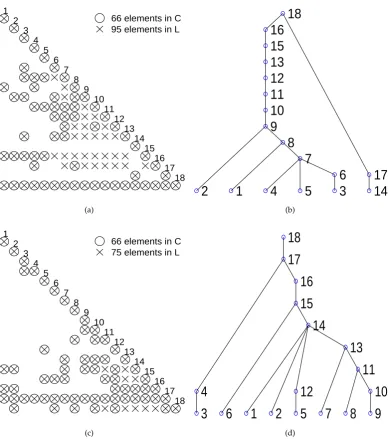
the parallelism as many as possible. Figure 1 compares the sparsity of theLDLTfactorLof a matrixC 130
and that of a reorder matrix. Here we employ the approximated minimum degree ordering [19] and
131
the parallel multi-frontalLDLTfactorization algorithm[20].
Algorithm 2 Newton-Raphson (NR)/Fisher Scoring (FS)/Averaged Information Splitting (AIS) method to solveS(θ) =0.
1: Give an initial guess ofθ0
2: for k=0, 1, 2,· · · until convergence do
3: Solve
IO(θk)δk=S(θk) for NR I(θk)δk =S(θk) for FS IA(θk)δk=S(θk) for AIS 4: θk+1=θk+δk
5: end for
Table 1. Date sets for the benchmark problem. The column titles are the number of years (y), the number of centres (c), the number of varieties(v), thes number of levels of cross terms(y.c , y.v, v.c), the average varieties per year (v/year), and the averages year per variety (y/v), and the number of controlled varieties all year (control varieties all year).
DataSet y c v y.c y.v v.c units v/y y/v c.v
prob_1 12 22 130 132 673 2518 6667 56.1 5.2 10
prob_2 15 25 160 180 888 3527 9595 59.2 5.6 10
prob_3 22 25 188 264 1177 4215 12718 53.5 6.3 12
prob_4 25 25 262 300 1612 5907 17420 64.5 6.2 12
prob_5 25 25 390 300 2345 8625 25334 93.8 6.0 15
prob_6 25 35 390 425 2345 12249 35887 93.8 6.0 15
prob_7 30 35 470 510 3013 15087 46113 100.4 6.4 20
prob_8 30 35 620 510 3835 19737 58685 127.8 6.2 20
prob_9 35 40 720 700 4522 26432 81396 129.2 6.3 20
prob_10 40 50 820 1000 5262 37701 118403 131.6 6.4 20
7. Numerical examples 133
A serial of plant breeding benchmark problems are used to verify performance of algorithms
134
implemented here. These examples are based on a second-stage analysis of a set of variety trials with
135
linear mixed models, i.e. based on variety predicted values from each trial. Trials are conducted in a
136
number of years across a number of locations (centres). The data in Table1are generated by a program
137
which allows you to specify the number of years, total number of centres and proportion of centres
138
used per year, the number of control varieties (used every year), the number of test varieties entering
139
the system per year and the average persistence of the test varieties, and the proportion of missing
140
varieties per trial, where proportions of things are selected. They are sampled at random, and the
141
life of each variety is generated from a Poisson distribution. This gives a three-way crossed structure
142
(year*variety*site) with some imbalance. In the current model, all terms except a grand mean are
143
fitted as random. The random terms are generated as independent and identically distributed normal
144
distribution with variance components generated from a test program with similar structure used for
145
the original SAS REML program, so it is just a variance components model.
146
The main part of the computing is the reordering and the factorization. Table2 compares the
147
algorithm implemented here and the counterpart in an existing commercial software, in which the
148
second column is the number of effects, third to fifth columns are speedup of algorithms implemented
149
here over the counterpart of an existing software package.
150
8. Discussion and future work 151
The aim of averaged information splitting is to remove computationally expensive and negligible
152
terms so that a simper approximate information matrix is obtained. Such a splitting keeps the
153
essential information and can be used as a good approximation to the observed information matrix
1 2
3 4
5 6
7 8
9 10
11 12
13 14
15 16
17 18 66 elements in C 95 elements in L
(a)
1
2
4
5
3
6
7
8
9
10
11
12
13
14
15
16
17
18
(b)
1 2
3 4
5 6
7 8
9 10
11 12
13 14
15 16
17 18 66 elements in C 75 elements in L
(c)
1
2
3
4
5
6
7
8
9
10
11
12
13
14
15
16
17
18
(d)
Figure 1.Illustration of the sparse structure of matrixCand its factorLin (a) and the sparse structure of the reordered matrix and its Cholesky factor L in (c). (b) and (d) are the elimination trees which indicate the elimination process correspond to the matrixCand its reordered matrix. The Cholesky elimination starts from a leaf node and ends in the root node. The height of he elimination tree stands for the sequential steps in the elimination, and the width of the elimination tree stands for the parallelism.
which is required for a derivative Newton method. The resulted formula is significantly simper
155
than that used in the software package used inNature Genetics[7, p.825, eq.8]. Together with the
156
fill-in reducing and multi-frontal factorization sparse matrix techniques, the splitting can significantly
157
improve the performance of a quasi-Newton approach to estimate the co-variance parameters
158
in the linear mixed models. Part of the result has been implemented in a leading commercial
159
breeding software package by VSN international(VSNi) Ltd. On a suit of test examples the method
160
described here ran 10 times faster than counterpart of VSNi’s existing software [18]. The splitting
161
approach builds up a framework to analysis unbalanced data sets modeled by liner mixed models.
162
Mathematically, theoretical proof on the convergence order of the quasi-Newton method based on the
Table 2.Speedup of of algorithms implemented here and the counterpart in an existing commercial software
prob No. of Effects Reordering Factorization all
Prob2 4796 * 25.98 6.46
Prob3 5892 15.4 * 4.95
Prob4 8132 14.78 * 7.55
Prob5 11711 12.32 * 6.65
Prob6 15470 15.15 8.91 7.16
Prob7 17.25 12.67 8.17
Prob8 24768 19.01 11.01 9.22
Prob9 32450 26.29 14.92 10.64
Prob10 44874 36.78 5.93 9.31
averaged information splitting deserves to be further investigated. It is of great interest to leverage
164
this method to actuarial science and other econometrics where the linear mixed models are used
165
intensively.
166
Acknowledgments:The project is supported by the Natural Science Fund of China(No.11501044) and partially 167
supported by NSFC(No.11571002, 11571047, 11671049, 11671051, 61672003). There is no funds for covering the 168
costs to publish in open access. 169
The founding sponsors had no role in the design of the study; in the collection, analyses, or
170
interpretation of data; in the writing of the manuscript, and in the decision to publish the results.
171
Bibliography 172
1. Patterson, H.D.; Thompson, R. Recovery of inter-block information when block sizes are unequal. 173
Biometrika1971,58, 545–554. 174
2. Masuda, Y.; Baba, T.; Suzuki, M. Application of supernodal sparse factorization and inversion to the 175
estimation of (co) variance components by residual maximum likelihood. Journal of Animal Breeding and 176
Genetics2013. 177
3. Bolker, B.M.e. Generalized linear mixed models:a practical guide for ecology and evolution. Trends in 178
Ecology and Evolution2008,24. 179
4. Lippert, C.; Listgarten, J.; Liu, Y.; Kadie, C.; Davidson, R.; Heckerman, D. FaST linear mixed models for 180
genome-wide association studies. Nature Methods2011,8, 833–835. 181
5. Listgarten, J.; Lippert, C.; Kadie, C.M.; Davidson, R.; Eskin, E.; Heckerman, D. Improved linear mixed 182
models for genome-wide association studies. Nature methods2012,9, 525–526. 183
6. Zhang, Z.; Ersoz, E.; Lai, C.Q.; Todhunter, R.; Tiwari, H.K.; Gore, M.; Bradbury, P.; Yu, J.; Arnett, D.; 184
Ordovas, J.; others. Mixed linear model approach adapted for genome-wide association studies. Nature 185
genetics2010,42, 355–360. 186
7. Zhou, X.; Stephens, M. Genome-wide efficient mixed-model analysis for association studies.Nature genetics 187
2012,44, 821–824. 188
8. Henderson,C.R.; Kempthorne, O.; Searle, S.R.; Krosigk,C. M. von. The estimation of environmental and 189
genetic trends from records subject to culling. Biometrics1959,15(2), 192–218. 190
9. Zhu,S.; Gu, T.; Xu, X; and Mo, Z Information splitting for big data analytics International Conference on 191
Cyber-enabled Distributed Computing and Knowledge Discoverybf 2016 294-302 192
10. Searle, S.R.; Casella, G; McCulloch, C.E. Variance components Wiley Series in Probability and Statisitcs. 193
John Wiley & Sons2006
194
11. Efron, B.; Hinkley, D. Assessing the accurancy of the maximum likelihood estimator:Observed versus 195
expected Fisher information.Biometrika1978,65, 457–487. 196
12. Misztal, I. Comparison of computing properties of derivative and derivative-free algorithms in 197
variance-component estimation by REML.Journal of Animal Breeding and Genetics1994,111, 346–355. 198
13. Jennrich, R.; Sampson, P. Newton-Raphson and related algorithms for maximum likelihood variance 199
14. Longford, N. A fast scoring algorithm for maximum likelihood estimation in unbalanced mixed models 201
with nested random effects.Biometrika1987,74, 817–827. 202
15. Johnson, D.L.; Thompson, R. Restricted maximum likelihood estimation of variance componnets for 203
univariate animal models using sparse matrix techniques and average information Journal of Dairy Science 204
1995,78(2), 449-456 205
16. Gilmour,A.R.; Thompson, R.; Cullis, B.R. Average information REML: An efficient algorithm for variance 206
parameter estimation in linear mixed models.Biometrics1995,51(4), 1440-1450 207
17. Zhu, S.; Gu, T.; Liu, X. Information matrix splitting.arXiv2016. arXiv:1605.07646v1. 208
18. Sue Welham, S.; Zhu, S.; Wathen, A.J. Big data, fast models: faster calculation of models from 209
high-throughput biological data sets. Knowledge Transfer Project Reprot IP12-009, Smith Industry 210
Mathematics Institute, The University of Oxford, Oxford, 2013. 211
19. Amestoy, P.R.; Davis, T.A.; Duff, I.S. An approximate minimum degree ordering algorithms SIAM Journal 212
on Matrix Analysis and Applications1996,17(4), 886-905 213
20. Davis, T.A. Algorithm 849: A concise sparse cholesky factroization package ACM Transactions on 214
Mathematical Software2005,31(4), 587-591 215
216