Unsteady MHD Flow Through Porous Medium In A Rotating Parallel Plate Channel Under The Influence Of Variable Pressure Gradient

(1)

Unsteady MHD Flow Through Porous Medium In A

Rotating Parallel Plate Channel Under The Influence Of

Variable Pressure Gradient

Shaik Sharmila

1

, Prof. R. Siva Prasad

1

1_{Department of Mathematics, Sri Krishnadevaraya University, Ananthapuramu-515003,}

Andhra Pradesh, India Email : [email protected]

Abstract:In this paper, an unsteady magneto hydro dynamic (MHD) two-layered fluids flow in a horizontal channel

between two parallel plates in the presence of an applied magnetic and electric field is investigated, when the whole system is rotated about an axis perpendicular to the flow. The flow is driven by a constant uniform pressure gradient in the channel bounded by two parallel insulating plates, when both fluids are considered as electrically conducting. The two fluids are assumed to be incompressible with variable properties, namely, different viscosities, thermal and electrical conductivities. Also, the transport properties of the two fluids are taken to be constant and the bounding plates are maintained at constant and equal temperatures. The governing partial differential equations are then reduced to the ordinary linear differential equations by using two-term series. Exact solutions for primary and secondary velocity distributions, also the temperatures are obtained in both fluid regions of the channel. Profiles of these solutions are plotted to discuss the effect on the flow and heat transfer characteristics, and their dependence on the governing parameters involved, such as the Hartmann number, Taylor number (rotation parameter), and ratios of the viscosities, heights, electrical and thermal conductivities. Moreover, an observation is made how the velocity and temperature distributions vary with hydro magnetic interaction in the case of steady and unsteady motions in the presence of rigid rotation.

Keywords: Porous Medium, Parallel Plate, Pressure Gradient, MHD

1. INTRODUCTION:

The flow of an electrically conducting fluid in the presence of a magnetic field is encountered in cosmical and geophysical fluid dynamics. The problems of fluid motion in parallel plate channels and rectangular channels have been studied by several authors due to their importance in engineering and

technological fields. Subsequently, considerable

attention has been also given to the study of magneto hydro dynamic flow of viscous fluids in a rotating system. New and emerging ideas have been added to the literature to possible applications in geophysics, astrophysics, engineering problems, geothermal energy, stem stimulation of oil field, food drying and heat pipes etc. The viscous fluid flow in a rotating frame of reference is of considerable importance due to the occurrence of various natural phenomena and for its application in various technological situations, which are governed by the actions of Coriolis forces.

The broad subjects of oceanography,

meteorology, atmospheric science and astronomy involve some important and essential features of rotating fluids. The rotating flow of an electrically conducting fluid in the presence of a magnetic field is encountered in cosmological and geophysical fluid dynamics. Many important observations on the viscous fluid flow problems in a rotating system under different conditions and configurations have come out from the analytical studies of many investigators, namely, Greenspan and Howard [13], Holton [20], Vidyanidhi [44], Walin [45], Siegman [40], Jana and Datta [22],

Seth et al. [38], Mazumder [29], Ganapathy [9], Hayat

et al.[18], Hayat and Hutter [16] and Das et al. [6]. The investigation on an oscillatory flow in a rotating channel is important from a practical point of view, because fluid oscillations may be expected in many MHD devices and natural phenomena where the fluid flow is generated due to the oscillating pressure gradient or due to vibrating plates/walls. In view of these facts, Mukherjee and Debnath [31], Seth and Jana [37], Singh [41], Ghosh [11], Ghosh and Pop [12] and Guria and Jana [14] investigated an oscillatory flow of a viscous incompressible electrically conducting fluid in a rotating channel under different conditions to analyze various aspects of the problem. Rahman and Sattar [33] studied an MHD free convection and mass transfer flow with an oscillating plate velocity and constant heat source in a rotating frame of reference.

(2)

Moreover, the temperature distribution plays an important role in MHD generators, plasma physics, turbines, etc. Also, it is a known fact that, to generate electricity, the temperature is used to run the turbine across a magnetic field. Transportation and extraction of the products of oil are other obvious applications using a two-phase system to obtain the increased flow rates in an electromagnetic pump from the possibility of reducing the power required to pump oil in a pipe line by a suitable addition of water (Shail, [39]).

There are several investigations with regards to both experimental and theoretical aspects of Magneto hydro dynamic flow problems, which are available in the literature [viz., Packham and Shail [32], Lielausis [23], Michiyoshi et al. [30], Chan [4], Chao et al. [5], Dunn [8], Gherson [10], Lohrasbi and Sahai [26],

Alireza and Sahai [1], Serizawa et al. [35], Malashetty

and Leela [27], Malashetty and Umavathi [28], Ramadan and Chamkha [3], Chamkha [2], Tsuyoshi Inoue and Shu-Ichiro Inutsuka [42] etc.]. Also, recent studies show that magneto hydro dynamic (MHD) flows can also be a viable option for transporting conducting fluids in micro scale systems, such as a flow inside the micro-channel networks of a lab-on-a-chip

device (Haim et al., [15]; Hussameddine et al., [21]. In

micro-fluidic devices, multiple fluids can be transported through a channel for different reasons. For example, an increase in mobility of a fluid may be achieved by stratification of a highly mobile fluid or mixing of two or more fluids in transit may be designed for emulsification or heat and mass transfer applications. In this regard, magnetic field-driven micro-pumps are an increasing demand due to their long-term reliability in generating flow, low power requirement and mixing

efficiency (Yi et al., [47] and Weston et al., [46]).

Most of the above investigations correspond to the steady flow situations. However, a significant number of practical problems dealing with immiscible fluids are unsteady in nature. In many practical problems, it is also advantageous to consider both immiscible fluids as electrically conducting, one of which is highly electrically conducting compared to the other. The fluid of low electrical conductivity compared to the other is helpful to reduce the power required to pump the fluid in MHD pumps and flow meters. In view of these facts, Heavy and Young [19] studied oscillating two-phase channel flows. Debnath and Basu [7] discussed the unsteady slip flow in an electrically conducting two-phase fluid under transverse magnetic fields. Chamkha [3] studied the unsteady MHD convective heat and mass transfer past a semi-infinite vertical permeable moving plate with heat absorption.

Umavathi et al. [43] investigated an oscillatory

Hartmann two-fluid flow and heat transfer in a horizontal channel. Linga Raju and Sreedhar [25] discussed an unsteady two-fluid flow and heat transfer of conducting fluids in channels under transverse magnetic field. On the other hand, the simultaneous influence of rotation and an external magnetic field on electrically conducting two-layered/two-phase fluid

systems seem to be dynamically important and physically useful etc.

2. FORMULATION AND SOLUTION:

Consider the unsteady MHD flow of a viscous incompressible electrically conducting fluid between two infinitely long horizontal parallel walls separated

by a distance h. Choose a Cartesian co-ordinates system

with the x-axis along the channel wall at y = 0, the y-

axis perpendicular to the channel walls and z-axis is

normal to the xy-plane as shown in the figure. 1. A

uniform transverse magnetic field H0 is applied

perpendicular to the channel walls. Since the channel walls are infinite in extent and the flow is unsteady, the

physical variables are the function of y and t only.

The unsteady governing equations of motion of the flow

through porous medium along x and z-directions in a

rotating frame of reference are

u

k

u

H

σμ

y

u

x

p

ρ

1

w

y

u

v

t

u

e

2





























2

0 2

0

2

(2.1)

w

k

w

H

σμ

y

w

u

y

w

v

t

w

_e

2























2

0 2

0

2

(2.2)

where, (u, w) is the velocity components along

O(x, z) directions respectively.



is the density of the

fluid,

μ

_e is the magnetic permeability,



is the

coefficient of kinematic viscosity, k is the permeability

of the medium,

H

₀ is the applied magnetic field and p

the fluid pressure. The initial and boundary conditions are

h

y

t

w

u



0

,



0

,



0

,

0



h

y

t

v

w

u



0

,



0

,



0

,



0

,



0

and



We introduce the non-dimensional variables

2 2 * 2 * 2 * * * * *

* _, _, _, _, _, _, _,

 

     

ph p h h

t t qh q wh w uh u h y y h x

x       

Making use of non-dimensional variables, the equations (2.1) and (2.2) becomes to (dropping asterisks)

Du

u

M

y

u

t

f

w

K

y

u

t

u

















2

2 2 2

)

(

2

Re

(2.4) Figure1: Physical Geometry of the problem

(3)

Dw

(Hartmann number squared)

2

(Rotation parameter),





(Non-dimensional pressure gradient)

Corresponding non-dimensional initial and boundary conditions are

1

Combining equations (2.4) and (2.5), Let

1

The initial and boundary conditions are

1

Taking the Laplace transform of the equation (2.7), we have

The transformed boundary conditions are

0

The solution of the equation (2.9) subjected to the boundary conditions (2.10) are

given by

P

are real constants.

Taking the inverse Laplace transforms to the equation (2.11), and we obtain the solution for the complex velocity q as,

2

K

. The equation (2.13) represents the velocity

of the fluid in the general case.

Now we shall consider the following special cases.

Case. 1. Velocity distribution for impulsive pressure gradient:

In this case

P

₁



P

₂



0

, then the equation (2.10)

reduces to

(4)

1

Case. 2. Velocity distribution for cosine oscillations of pressure gradient:

In this case

P

₀



0

and

Case. 3. Velocity distribution for sine oscillations of pressure gradient:

In this case

P

₀



0

and

Shear Stress:

For the impulsive change of pressure gradient, the

non-dimensional shear stresses at the wall

y



0

are given

by

For the cosine oscillations of pressure gradient, the

non-dimensional shear stresses at the wall

y



0

are given

(5)





For the sine oscillations of pressure gradient, the non-dimensional shear stresses at the

wall

y



0

are given by

3. RESULTS AND DISCUSSION

The unsteady MHD flow of a viscous incompressible electrically conducting fluid through porous medium in a rotating parallel plate channel with

variable pressure gradient has been studied. The governing equations are solved analytically using the Laplace transform technique. For computationally we have considered three different cases 1. Impulsive change of pressure gradient, 2. Cosine oscillations of pressure gradient and 3. Sine oscillations of pressure gradient. The flow governed by the non-dimensional

parameters for the velocity components u and w with

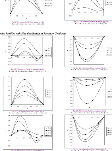
impulsive pressure gradient Fig.10-Fig.21 represent the velocity profiles for cosine oscillations of pressure gradient, where as the Fig.22-Fig.33 represent the velocity profiles for sine oscillations of pressure gradient.

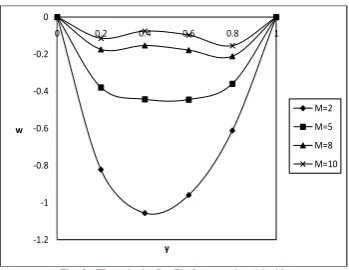
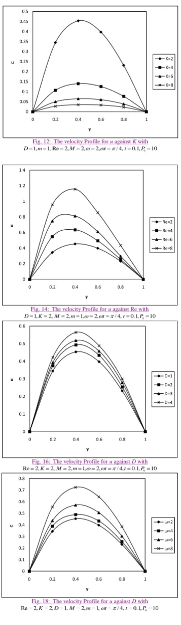
We have seen from Fig.2, Fig.10 and Fig.22

that the velocity component u increases with an increase

in magnetic parameter M for the impulsive change, and

decreases for cosine and sine oscillations of the pressure gradient. Fig.3, Fig.11 and Fig.23 shows that the

velocity component w decreases for the cosine

oscillations of the pressure gradient while it increases for impulsive change and sine oscillations of the

secondary velocity w decreases for cosine oscillations

of the pressure gradient, while primary velocity u

increases and w reduces throughout the fluid region

with an increase in rotation parameter K for impulse

change, the reversal behaviour is observed for sine oscillations of the pressure gradient. The rotation parameter defines the relative magnitude of the Coriolis force and the viscous force in the regime; therefore it is clear that high magnitude Coriolis forces are counter-productive for the primary flow. Fig.6, Fig.14 and

Fig.26, we noticed that the primary velocity u decreases

with an increase in Reynolds number Re for the impulsive change, while it increases with an increase in Reynolds number Re for cosine oscillations of the pressure gradient, the magnitude of the velocity

component w enhances initially for

y



0

.

2

and then

gradually reduces for

0

.

4



y



1

with an increase in

Reynolds number Re for sine oscillations of the pressure gradient.

It is seen from Fig.7, Fig.15 and Fig.27 that the

secondary velocity w increases for the impulsive change

while it decreases for sine oscillations of the pressure gradient with an increase in Reynolds number Re.

Similarly, the magnitude of the velocity component w

enhances initially for

y



0

.

2

and then gradually

(6)

number Re for cosine oscillations of the pressure gradient. It is seen from Fig.8, Fig.16, and Fig.28 that

the primary velocity u increases with an increase in

permeability parameter D for the impulsive change,

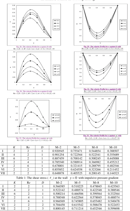
cosine and sine oscillations of the pressure gradient throughout the fluid region. Likewise from Fig.9,

Fig.17 and Fig.29 that the secondary velocity w reduces

with an increase in permeability parameter D for sine

oscillations of the pressure gradient while it enhances for the impulsive change and cosine oscillations of the pressure gradient. Fig.18 and Fig.30 shown that the

primary velocity u increases with an increase in

frequency parameter



for cosine oscillations of the

pressure gradient while the velocity u enhances for

6

&

4

,

2





and then experiences retardation for

8





for sine oscillations of the pressure gradient. It

has been seen from Fig.15 and Fig.31 that the

secondary velocity w decreases for the sine oscillations

of the pressure gradient while the velocity u enhances

for





2

,

4

&

6

8





for cosine oscillations of the pressure gradient

with an increase in frequency parameter



. Finally we

have noticed from Fig.20 and Fig.32 that, the

magnitude of the primary velocity u decreases with an

increase in phase angle



t

for both cosine and sine

oscillations of the pressure gradient. It is also seen from

Fig.21 and Fig.33 that the secondary velocity w reduces

for cosine oscillations of the pressure gradient while it increases for sine oscillations of the pressure gradient

with an increase in phase angle



t

. It is noted that, the

magnitude of the velocities for cosine oscillations of the pressure gradient are always greater than magnitude of sine oscillations of the pressure gradient.

The non-dimensional shear stresses



_x and



_z

have been calculated at the wall (

y



0

) due to the

primary and the secondary flows are presented in Table1-Table6 and computationally discussed with reference to governing parameters like, magnetic

parameter M, rotation parameter K, Reynolds number

Re, Permeability parameter D, frequency parameter



and phase angle



t

. We notice that the shear stresses

x



and



_z due to the primary and secondary flow at the

wall

y



0

reduce for the impulsive change, cosine and

sine oscillations of the pressure gradient with an

increase in Hartmann number M. The magnitude of

the shear stress



_x due to the primary flow decreases

for the impulsive change and cosine oscillations, while it increases for sine oscillations of the pressure gradient

with an increase in rotation parameter K or Permeability

parameter D. It is found that the shear stress



_z

decreases for both impulsive change and cosine oscillations of the pressure gradient while it increases for sine oscillations of the pressure gradient with an

increase in rotation parameter K and Permeability

parameter D. The shear stress



_x decreases for small

values of magnetic parameter M (



8) and then it

increases for the impulsive change, cosine and sine oscillations of the pressure gradient with an increase in

Reynolds number Re. Also the shear stress



_z increases

for both impulsive change and cosine oscillations of the pressure gradient while it decreases for sine oscillations of the pressure gradient with an increase in Reynolds

number Re. The shear stress



_x increases for small



8) and then it

decreases for cosine and sine oscillations of the pressure

gradient with an increase in frequency parameter



. It

is found that the shear stress



_z increases for small



8) and then it

decreases for cosine oscillations while it first decreases and then increases for sine oscillations of the pressure

gradient with an increase in frequency parameter



.

The shear stress



_x decreases for both cosine and sine

oscillations of the pressure gradient with an increase in

phage angle



t

. Also the shear stress



_z decreases for

cosine oscillations of the pressure gradient while it increases for sine oscillations of the pressure gradient

with an increase in phage angle



t

.

4. GRAPHS & TABLES

I. Velocity Profiles with Impulsive Pressure Gradient:

Fig. 2: The velocity Profile for u against M with

10 , 1 . 0 , 1 , 2 Re , 2 ,

1     0

 K m t P

D 0 1 2 3 4 5 6

0 0.2 0.4 0.6 0.8 1

u

y

M=2

M=5

M=8

M=10

Fig. 3: The velocity Profile for w against M with

10 , 1 . 0 , 1 , 2 Re , 2 ,

1     0

 K m t P

D -1.2

-1 -0.8 -0.6 -0.4 -0.2 0

0 0.2 0.4 0.6 0.8 1

w

y

M=2

M=5

M=8

(7)

Fig. 4: The velocity Profile for u against K with

10 , 1 . 0 , 2 , 2 Re , 1 ,

1     0

 m M t P

D 0 0.5 1 1.5 2 2.5 3 3.5 4

0 0.2 0.4 0.6 0.8 1

u

y

K=2

K=4

K=6

K=8

Fig. 5: The velocity Profile for w against K with 10 , 1 . 0 , 2 , 2 Re , 1 ,

1     0

 m M t P D

-2.5 -2 -1.5 -1 -0.5 0

0 0.2 0.4 0.6 0.8 1

w

y

K=2 K=4 K=6 K=8

Fig. 6: The velocity Profile for u against Re with

10 , 1 . 0 , 1 , 2 , 2 ,

1     0

 K M m t P

D 0 0.2 0.4 0.6 0.8 1 1.2 1.4 1.6 1.8

0 0.2 0.4 0.6 0.8 1

u

y

Re=2

Re=4

Re=6

Re=8

Fig. 7: The velocity Profile for w against Re with

10 , 1 . 0 , 1 , 2 , 2 ,

1     0

 K M m t P

D -1.2

-1 -0.8 -0.6 -0.4 -0.2 0

0 0.2 0.4 0.6 0.8 1

w

y

Re=2

Re=4

Re=6

Re=8

Fig. 8: The velocity Profile for u against D with 10 , 1 . 0 , 1 , 2 , 2 , 2

Re K M m t P0

0 0.5 1 1.5 2 2.5 3

0 0.2 0.4 0.6 0.8 1

u

y

D=1 D=2 D=3 D=4

Fig. 9: The velocity Profile for w against D with

10 , 1 . 0 , 1 , 2 , 2 , 2

Re K M m t P0

-1.2 -1 -0.8 -0.6 -0.4 -0.2 0

0 0.2 0.4 0.6 0.8 1

w

y

D=1

D=2

D=3

D=4

II. Velocity Profiles with Cosine Oscillation of Pressure Gradient:

10 , 1 . 0 , 4 / , 2 , 1 , 2 Re , 2 ,

1       0

 K m t t P

D   

0 0.05 0.1 0.15 0.2 0.25 0.3 0.35 0.4 0.45 0.5

0 0.2 0.4 0.6 0.8 1

u

y

M=2

M=5

M=8

M=10

10 , 1 . 0 , 4 / , 2 , 1 , 2 Re , 2 ,

1       0

 K m t t P

D   

-0.06 -0.04 -0.02 0 0.02 0.04 0.06 0.08 0.1 0.12

0 0.2 0.4 0.6 0.8 1

w

y

(8)

Fig. 12: The velocity Profile for u against K with

10 , 1 . 0 , 4 / , 2 , 2 , 2 Re , 1 ,

1       0

 m M t t P

D   

0 0.05 0.1 0.15 0.2 0.25 0.3 0.35 0.4 0.45 0.5

0 0.2 0.4 0.6 0.8 1

u

y

K=2

K=4

K=6

K=8

Fig. 13: The velocity Profile for w against K with

10 , 1 . 0 , 4 / , 2 , 2 , 2 Re , 1 ,

1       0

 m M t t P

D   

0 0.02 0.04 0.06 0.08 0.1 0.12

0 0.2 0.4 0.6 0.8 1

w

y

K=2

K=4

K=6

K=8

10 , 1 . 0 , 4 / , 2 , 1 , 2 , 2 ,

1       0

 K M m t t P

D   

0 0.2 0.4 0.6 0.8 1 1.2 1.4

0 0.2 0.4 0.6 0.8 1

u

y

Re=2

Re=4

Re=6

Re=8

10 , 1 . 0 , 4 / , 2 , 1 , 2 , 2 ,

1       0

 K M m t t P

D   

-0.2 -0.1 0 0.1 0.2 0.3 0.4

0 0.2 0.4 0.6 0.8 1

w

y

Re=2

Re=4

Re=6

Re=8

Fig. 16: The velocity Profile for u against D with

10 , 1 . 0 , 4 / , 2 , 1 , 2 , 2 , 2

Re K M m  t t P0

0 0.1 0.2 0.3 0.4 0.5 0.6

0 0.2 0.4 0.6 0.8 1

u

y

D=1

D=2

D=3

D=4

Fig. 17: The velocity Profile for w against D with

10 , 1 . 0 , 4 / , 2 , 1 , 2 , 2 , 2

Re K M m  t t P0

0 0.02 0.04 0.06 0.08 0.1 0.12 0.14 0.16 0.18

0 0.2 0.4 0.6 0.8 1

w

y

D=1 D=2 D=3 D=4

10 , 1 . 0 , 4 / , 1 , 2 , 1 , 2 , 2

Re K D M m t t P0

0 0.1 0.2 0.3 0.4 0.5 0.6 0.7 0.8

0 0.2 0.4 0.6 0.8 1

u

y

ω=2

ω=4

ω=6

ω=8

Fig. 19: The velocity Profile for w against D with 10 , 1 . 0 , 4 / , 1 , 2 , 2 , 2

Re K M m t t P0

0 0.05 0.1 0.15 0.2 0.25 0.3

0 0.2 0.4 0.6 0.8 1

w

y

(9)

Fig.20 The velocity Profile for u against t with

10 , 1 . 0 , 2 , 1 , 2 , 2 , 2

Re K M m  t P0

0 0.1 0.2 0.3 0.4 0.5 0.6

0 0.2 0.4 0.6 0.8 1

u

y

ωt=π/6

ωt=π/4

ωt=π/3

Fig. 21: The velocity Profile for w against t with 10 , 1 . 0 , 2 , 1 , 2 , 2 , 2

Re K M m  t P0

-0.05 0 0.05 0.1 0.15 0.2

0 0.2 0.4 0.6 0.8 1

w

y

ωt=π/6

ωt=π/4

ωt=π/3

III. Velocity Profiles with Sine Oscillation of Pressure Gradient:

10 , 1 . 0 , 4 / , 2 , 1 , 2 Re , 2 ,

1       0

 K m t t P

D   

-0.06 -0.04 -0.02 0 0.02 0.04 0.06 0.08 0.1 0.12

0 0.2 0.4 0.6 0.8 1

u

y

M=2

M=5

M=8

M=10

10 , 1 . 0 , 4 / , 2 , 1 , 2 Re , 2 ,

1       0

 K m t t P

D   

-0.5 -0.45 -0.4 -0.35 -0.3 -0.25 -0.2 -0.15 -0.1 -0.05 0

0 0.2 0.4 0.6 0.8 1

w

y

M=2 M=5 M=8 M=10

Fig. 24: The velocity Profile for u against K with 10 , 1 . 0 , 4 / , 2 , 2 , 2 Re , 1 ,

1       0

 m M t t P

D   

0 0.02 0.04 0.06 0.08 0.1 0.12

0 0.2 0.4 0.6 0.8 1

u

y

K=2 K=4 K=6 K=8

Fig. 25: The velocity Profile for w against K with

10 , 1 . 0 , 4 / , 2 , 2 , 2 Re , 1 ,

1       0

 m M t t P

D   

-0.5 -0.45 -0.4 -0.35 -0.3 -0.25 -0.2 -0.15 -0.1 -0.05 0

0 0.2 0.4 0.6 0.8 1

w

y

K=2

K=4

K=6

K=8

10 , 1 . 0 , 4 / , 2 , 1 , 2 , 2 ,

1       0

 K M m t t P

D   

-0.2 -0.1 0 0.1 0.2 0.3 0.4

0 0.2 0.4 0.6 0.8 1

u

y

Re=2

Re=4

Re=6

Re=8

10 , 1 . 0 , 4 / , 2 , 1 , 2 , 2 ,

1       0

 K M m t t P

D   

-1 -0.9 -0.8 -0.7 -0.6 -0.5 -0.4 -0.3 -0.2 -0.1 0

0 0.2 0.4 0.6 0.8 1

w

y

(10)

10 , 1 . 0 , 4 / , 2 , 1 , 2 , 2 , 2

Re K M m  t t P0

0 0.02 0.04 0.06 0.08 0.1 0.12 0.14 0.16 0.18

0 0.2 0.4 0.6 0.8 1

u

y

D=1

D=2

D=3

D=4

Fig. 29: The velocity Profile for w against D with

10 , 1 . 0 , 4 / , 2 , 1 , 2 , 2 , 2

Re K M m  t t P0

-0.6 -0.5 -0.4 -0.3 -0.2 -0.1 0

0 0.2 0.4 0.6 0.8 1

w

y

D=1 D=2 D=3 D=4

10 , 1 . 0 , 4 / , 1 , 2 , 1 , 2 , 2

Re K D M m t t P0

0 0.05 0.1 0.15 0.2 0.25 0.3

0 0.2 0.4 0.6 0.8 1

u

y

ω=2

ω=4

ω=6

ω=8

Fig. 31: The velocity Profile for w against D with 10 , 1 . 0 , 4 / , 1 , 2 , 2 , 2

Re K M m t t P0

-0.8 -0.7 -0.6 -0.5 -0.4 -0.3 -0.2 -0.1 0

0 0.2 0.4 0.6 0.8 1

w

y

ω=2

ω=4

ω=6

ω=8

Fig. 32: The velocity Profile for u against t with

10 , 1 . 0 , 2 , 1 , 2 , 2 , 2

Re K M m  t P0

-0.05 0 0.05 0.1 0.15 0.2

0 0.2 0.4 0.6 0.8 1

u

y

ωt=π/6

ωt=π/4

ωt=π/3

Fig. 33: The velocity Profile for w against t with 10 , 1 . 0 , 2 , 1 , 2 , 2 , 2

Re K M m  t P0

-0.6 -0.5 -0.4 -0.3 -0.2 -0.1 0

0 0.2 0.4 0.6 0.8 1

w

y

ωt=π/6

ωt=π/4

ωt=π/3

K Re D M=2 M=5 M=8 M=10

I 2 2 1 0.920545 0.755471 0.544854 0.388507

II 4 2 1 0.901254 0.722564 0.522541 0.355689

III 6 2 1 0.887459 0.700142 0.500245 0.445088

IV 2 4 1 0.785540 0.588914 0.366982 0.455212

V 2 6 1 0.678801 0.321415 0.288795 0.482546

VI 2 2 2 0.855852 0.624558 0.323266 0.211452

VII 2 2 3 0.648878 0.405525 0.200145 0.144523

Table 1: The shear stress (



_x) at the wall

y



0

with impulsive pressure gradient

K Re D M=2 M=5 M=8 M=10

I 2 2 1 0.566585 0.510225 0.478845 0.425563

II 4 2 1 0.522142 0.488574 0.422548 0.388546

III 6 2 1 0.500214 0.466506 0.399564 0.332564

IV 2 4 1 0.788548 0.622564 0.578045 0.488574

V 2 6 1 0.966569 0.745805 0.655482 0.540478

VI 2 2 2 0.704458 0.615542 0.588478 0.522453

VII 2 2 3 0.800145 0.711214 0.652546 0.599698

(11)

K Re D



t

M=2 M=5 M=8 M=10

I 2 2 1 2



/

4

0.814025 0.755845 0.681452 0.622142

II 4 2 1 2



/

4

0.722459 0.699857 0.640563 0.574486

III 6 2 1 2



/

4

0.622546 0.584740 0.589902 0.510252

IV 2 4 1 2



/

4

0.788458 0.685548 0.622548 0.684476

V 2 6 1 2



/

4

0.688982 0.566809 0.566527 0.722105

VI 2 2 2 2



/

4

0.699885 0.685041 0.661245 0.600732

VII 2 2 3 2



/

4

0.588987 0.562215 0.541046 0.522146

VIII 2 2 1 4



/

4

0.998702 0.855406 0.746025 0.520214

IX 2 2 1 6



/

4

1.225473 0.958456 0.866502 0.445106

X 2 2 1 2



/

6

0.885442 0.822546 0.755480 0.688549

XI 2 2 1 2



/

3

0.745582 0.722152 0.622548 0.588479



_x) at the wall

y



0

with cosine oscillations of

pressure gradient



_z) at the wall

y



0

with cosine oscillations of

pressure gradient

K Re D



t

M=2 M=5 M=8 M=10

I 2 2 1 2



/

4

0.356636 0.322546 0.299555 0.277485

II 4 2 1 2



/

4

0.388546 0.352262 0.314452 0.299873

III 6 2 1 2



/

4

0.399658 0.366585 0.322506 0.302145

IV 2 4 1 2



/

4

0.321021 0.302589 0.288695 0.266899

V 2 6 1 2



/

4

0.301332 0.284585 0.266554 0.244855

VI 2 2 2 2



/

4

0.366525 0.336502 0.300045 0.299845

VII 2 2 3 2



/

4

0.377785 0.344215 0.321787 0.332566

VIII 2 2 1 4



/

4

0.255466 0.210023 0.199665 0.156656

IX 2 2 1 6



/

4

0.221455 0.188545 0.144526 0.122546

X 2 2 1 2



/

6

0.422515 0.400526 0.355626 0.322145

XI 2 2 1 2



/

3

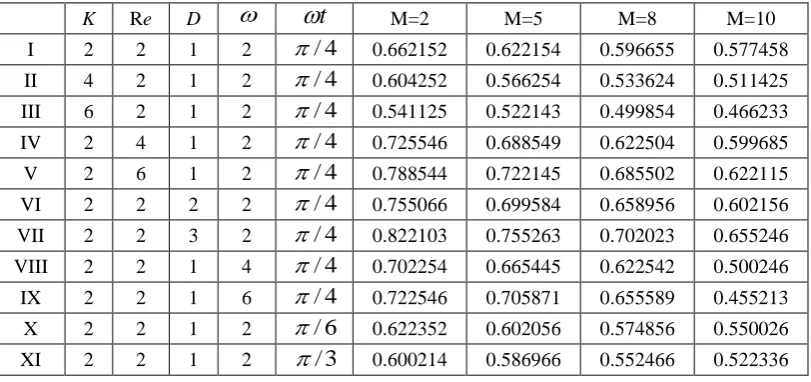
0.333256 0.302214 0.255664 0.221552



_x) at the wall

y



0

with sine oscillations of

pressure gradient

K Re D



t

M=2 M=5 M=8 M=10

I 2 2 1 2



/

4

0.662152 0.622154 0.596655 0.577458

II 4 2 1 2



/

4

0.604252 0.566254 0.533624 0.511425

III 6 2 1 2



/

4

0.541125 0.522143 0.499854 0.466233

IV 2 4 1 2



/

4

0.725546 0.688549 0.622504 0.599685

V 2 6 1 2



/

4

0.788544 0.722145 0.685502 0.622115

VI 2 2 2 2



/

4

0.755066 0.699584 0.658956 0.602156

VII 2 2 3 2



/

4

0.822103 0.755263 0.702023 0.655246

VIII 2 2 1 4



/

4

0.702254 0.665445 0.622542 0.500246

IX 2 2 1 6



/

4

0.722546 0.705871 0.655589 0.455213

X 2 2 1 2



/

6

0.622352 0.602056 0.574856 0.550026

(12)

K Re D



t

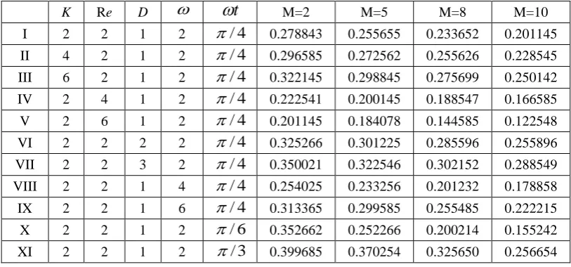
M=2 M=5 M=8 M=10

I 2 2 1 2



/

4

0.278843 0.255655 0.233652 0.201145

II 4 2 1 2



/

4

0.296585 0.272562 0.255626 0.228545

III 6 2 1 2



/

4

0.322145 0.298845 0.275699 0.250142

IV 2 4 1 2



/

4

0.222541 0.200145 0.188547 0.166585

V 2 6 1 2



/

4

0.201145 0.184078 0.144585 0.122548

VI 2 2 2 2



/

4

0.325266 0.301225 0.285596 0.255896

VII 2 2 3 2



/

4

0.350021 0.322546 0.302152 0.288549

VIII 2 2 1 4



/

4

0.254025 0.233256 0.201232 0.178858

IX 2 2 1 6



/

4

0.313365 0.299585 0.255485 0.222215

X 2 2 1 2



/

6

0.352662 0.252266 0.200214 0.155242

XI 2 2 1 2



/

3

0.399685 0.370254 0.325650 0.256654



_z) at the wall

y



0

with sine oscillations of pressure gradient

5. CONCLUSIONS:

 The velocity component for primary flow

enhances with increasing M, K and D, and

reduces with Re for the impulsive change of pressure gradient.

 The velocity component for secondary flow

enhances with increasing M, Re and D, and

reduces with K for the impulsive change of

pressure gradient.

increases with increasing Re, D and



, and

reduces with M, K and phase angle



t

for the

cosine oscillations of pressure gradient.

increases with increasing D, and reduces with

M, K and phase angle



t

for the sine

oscillations of pressure gradient.

 The magnitude of the velocity components for

primary flow and for secondary flow enhances

initially for

y



0

.

2

and then gradually

reduces for

0

.

2



y



1

with an increase in

Reynolds number Re for sine and cosine

oscillations of the pressure gradient

respectively.

 The velocity for primary flow and for

secondary flow enhances for





2

,

4

&

6





8

for

sine and cosine oscillations of the pressure gradient respectively.

 The velocity component for secondary flow

enhances with increasing M, K and phase angle

t



, and reduces with increase in Re, D and

frequency of oscillation



for the impulsive

change of pressure gradient.

 The magnitude of the shear stress



_x due to

the primary flow decreases for the impulsive change and cosine of the pressure gradient

with an increase in M, Re, K or Permeability

parameter D.

 The magnitude of the shear stress



_z due to

the secondary flow reduces for the impulsive change and cosine of the pressure gradient

with an increase in rotation parameter M or K

and enhances with increasing in Re or D.

 Both the stresses enhance with increase in K

and D; and reduce with increase in M or Re for

sine of the pressure gradient.

 The shear stress



_x increases for small values

of magnetic parameter M (



8) and then it

decreases for cosine and sine oscillations of the pressure gradient with an increase in

frequency parameter



.



_z increases for small values

of magnetic parameter M (



8) and then it

decreases for cosine oscillations while it first decreases and then increases for sine oscillations of the pressure gradient with an

increase in frequency parameter



.



_x decreases for both cosine

and sine oscillations of the pressure gradient

with an increase in phage angle



t

. Also the

shear stress



_z decreases for cosine

oscillations of the pressure gradient while it increases for sine oscillations of the pressure

gradient with an increase in phage angle



t

.

REFERENCES:

[1]. Alireza S. and Sahai V. Heat transfer in

developing magnetohydrodynamic

poiseuille flow and variable Transport properties, International Journal of Heat Mass Transfer, vol.33 (8), pp.1711-1720(1990).

[2]. Chamkha A.J. Flow of two-immiscible fluids in

(13)

of Fluids Engineering, vol.122, pp.117-124(2000).

[3]. Chamkha A.J. Unsteady MHD convective heat

and mass transfer past a semi-infinite vertical permeable moving plate with heat absorption,

International Journal of

Engineering Science, vol.42, pp.217-230(2004).

[4]. Chan C.K. Finite element formulation and

solution of nonlinear heat transfer, Journal of Nuclear Engineering and Design, vol.51, p.253 (1979).

[5]. Chao J., Mikic B.B. and Todreas N.E. Radiation

streaming in power reactors: proceedings of the special session, American Nuclear Society (ANS) Winter Meeting, Washington, D.C. Nuclear Technology, 42, 22(1979).

[6]. Das B.K., Guria M. and Jana R.N. Unsteady

Couette flow in a rotating system, Meccanica, vol.43, p.517|(2008).

[7]. Debnath L. and Basu U. Unsteady slip flow in an

electrically conducting two-phase fluid under transverse magnetic fields, Nuovo Cimento, vol.28B,pp.349-362(1975).

[8]. Dunn P.F. Single-phase and two-phase magneto

hydro dynamic pipe flow, International Journal of Heat Mass Transfer, vol.23, p.373 (1980).

[9]. Ganapathy R. A note on oscillatory Couette flow

in a rotating system. ASME, Journal of Applied Mechanics, vol.61, p.208 (1994).

[10].Gherson P. and Lykoudis P.S. Local

measurements in two-phase liquid-metal

magneto-fluid mechanic flow, Journal of Fluid Mechanics, vol.147, pp.81-104(1984).

[11].Ghosh S.K. Unsteady hydromagnetic flow in a

rotating channel with oscillating pressure gradient, Journal of the Physical Society of Japan, vol.62, p.3893 (1993).

[12].Ghosh S.K. and Pop I. Hall effects on unsteady

hydro magnetic flow in a rotating system with

oscillatory pressure gradient, International

Journal of Applied Mechanics and Engineering, vol.8, p.43 (2003).

[13].Greenspan H.P. and Howard L.N. On a time

dependent motion of a rotating fluid, Journal of Fluid Mechanics, vol.17, p.385 (1963).

[14].Guria M. and Jana R.N. Hydro magnetic flow in

the Ekman layer on an oscillating porous plate. Magneto hydro dynamics , vol.43, pp.3-11(2007).

[15].Haim H.B., Jianzhong Z., Shizhi Q. and Yu X. A

magneto-hydrodynamically controlled fluidic network, Sensors and Actuators B, vol.88 (2), pp.205–216(2003).

[16].Hayat T. and Hutter K. Rotating flow of a

second-order fluid on a porous plate,

International Journal of Non-Linear Mechanics, vol.39, p.767 (2004).

[17].Hayat T., Nadeem S. and Asghar S.

Hydromagnetic Couette flow of an Oldroyd-B

fluid in a rotating system , International Journal of Engineering Science, vol.42, p.65 (2004).

[18].Hayat T., Nadeem S., Asghar S. and Siddiqui

A.M. Fluctuating flow of a third-grade fluid on a porous plate in a rotating medium, International Journal of Non-Linear Mechanics, vol.36, p.901 (2001).

[19].Heavy J.V. and Young H.T. Oscillating two-

phase channel flows, Z. Angew. Math. Phys.,vol.21, p.454 (1970).

[20].Holton J. R. The influence of viscous boundary

layers on transient motions in a stratified rotating fluid, International Journal of Atmospheric Science, vol.22, p.402 (1965).

[21].Hussameddine S.K.,Martin J.M. and Sang W.J.

Analytical prediction of flow field in magneto hydro dynamic based micro fluidic devices, Journal of Fluids Engineering, vol.130(9), p.6(2008).

[22].Jana R.N. and Datta N. Couette flow and heat

transfer in a rotating system Acta

Mechanica,vol.26, p.301 (1977).

[23].Lielausis O. Liquid metal magneto

hydrodynamics, Atomic Energy Review, vol.13, p.527 (1975).

[24].Linga Raju T. and Murty P.S.R. Hydro magnetic

two-phase flow and heat transfer through two parallel plates in a rotating system Journal of Indian Academy of Mathematics, Indore, India, vol.28 (2), pp.343-360(2006).

[25].Linga Raju T. and Sreedhar S. Unsteady

two-fluid flow and heat transfer of conducting two-fluids in channels under transverse magnetic field International Journal of Applied Mechanics and Engineering, vol.14(4), pp.1093-1114(2009).

[26].Lohrasbi J. and Sahai V. Magnetohydrodynamic

heat transfer in two-phase flow between parallel plates Applied Scientific Research, vol.45, pp.53-66(1989).

[27].Malashetty M.S. and Leela V.

Magnetohydrodynamic heat transfer in two phase flow International Journal of Engineering Science, vol.30, pp.371-377(1992).

[28].Malashetty M.S. and Umavathi J.C. Two phase

magneto hydrodynamic flow and heat

transfer in an inclined channel International Journal of Multiphase Flow, vol.23 (3), pp.545-560(1997).

[29].Mazumder B.S. An exact solution of oscillatory

Couette flow in a rotating system ASME Journal of Applied Mechanics, vol.58, p.1104 (1991).

[30].Michiyoshi Funakawa Kuramoto C., Akita Y.

and Takahashi O. Instead of the helium-lithium annular mist flow at high temperature, an

air-mercury stratified flow in a horizontal

(14)

[31].Mukherjee S. and Debnath L. On unsteady rotating boundary layer flows between two porous plates ZAMM, vol.57, p.188 (1977).

[32].Packham B.A. and Shail R. Stratified laminar

flow of two immiscible fluids. Proceedings of

Cambridge Philosophical Society, vol.69,

pp.443-448(1971).

[33].Rahman M.M. and Sattar M.A. MHD free

convection and mass transfer flow with oscillating plate velocity and constant heat source in a rotating frame of reference, The Dhaka University Journal of Science, vol.47, p.63(1999).

[34].Ramadan H.M. and Chamkha A.J. Two-phase

free convection flow over an infinite permeable inclined plate with non-uniform particle-phase density, International Journal of Engineering Science, vol.37, p.1351 (1999).

[35].Serizawa A., Ida T., Takahashi O. and

Michiyoshi I.MHD effect on Nak-nitrogen two-phase flow and heat transfer in a vertical round

tube International Journal Multi-Phase

Flow,vol.16 (5), p.761 (1990).

[36].Seth G.S. and Ansari M.S. Magneto hydro

dynamic convective flow in a rotating channel with Hall effects International Journal of Theoretical and Applied Mechanics, vol.4, p.205 (2009).

[37].Seth G.S. and Jana R.N.Unsteady hydro

magnetic flow in a rotating channel with oscillating pressure gradient Acta Mechanica, vol.37, p.29 (1980).

[38].Seth G.S., Jana R.N. and Maiti M.K. Unsteady

hydro magnetic Couette flow in a rotating system International Journal of Engineering Science, vol.20, p.989 (1982).

[39].Shail R. On laminar tow-phase flow in magneto

hydro dynamics International Journal of

Engineering Science, vol.11, p.1103 (1973).

[40].Siegmann W.L. The spin-down of rotating

stratified fluids Journal of Fluid

Mechanics,vol.47, p.689 (1971).

[41].Singh K.D. An oscillatory ydromagnetic Couette

flow in a rotating system ZAMM,

vol.80, p.429 (2000).

[42].Tsuyoshi I. and Shu-Ichiro I. Two-fluid magneto

hydrodynamic simulation of converging Hi flows in the Interstellar medium The Astrophysical Journal, vol.687(1), pp.303-310(2008).

[43].Umavathi J.C., Abdul Mateen, Chamkha A.J.

and Al- Mudhaf A. Oscillatory Hartmann two-fluid flow and heat transfer in a horizontal

channel International Journal of Applied

Mechanics and Engineering, vol.11 (1), pp.155-178(2006).

[44].Vidyanidhi V. Secondary flow of a conducting

liquid in a rotating channel Journal of Mathematical and Physical Sciences, vol.3, p.193 (1969).

[45].Walin G. Some aspects of time dependent

motion of a stratified rotating fluid Journal of Fluid Mechanics, vol.36, p.289 (969).

[46].Weston M.C., Gerner M.D. and Fritsch I.

Magnetic fields for fluid motion Analytical Chemistry, vol.82 (9), pp.3411–3418(2010).

[47].Yi M., Qian S. and Bau H. A magneto hydro