Neural Network Classifiers for Human Tissue Classification in NIR Biomedical Multispectral Imaging

(1)

Neural Network Classifiers for

Human Tissue Classification in NIR

Biomedical Multispectral Imaging

by

Sandeep Gurm

A thesis

presented to the University of Waterloo in fulfillment of the

thesis requirement for the degree of Master of Applied Science

in

Systems Design Engineering

Waterloo, Ontario, Canada, 2018

c

(2)

This thesis consists of material all of which I authored or co-authored: see Statement of Contributions included in the thesis. This is a true copy of the thesis, including any required final revisions, as accepted by my examiners.

(3)

Statement of Contributions

Content from the following paper is used in this thesis in Chapter 5:

Gurm, Sandeep, Ossama Badawy, and Alexander Wong. ”A Multi-layer Perceptron Approach to Automatically Detect Tissue via NIR Multispectral Imaging.” Journal of Computational Vision and Imaging Systems 3.1 (2017).

Contributor Statement of Contribution

S. Gurm (Candidate)

Conceptual Design - 100%

Data Collection and Analysis - 90% Writing and Editing - 70%

A. Wong Data Collection and Analysis - 10% Writing and Editing - 20%

(4)

Abstract

Near infrared imaging (NIR) is an imaging modality that has gained traction for solving biomedical problems in recent years. By leveraging the NIR spectrum, multiple spectra from the NIR range can be used to extract meaningful data from a variety of targets including human tissue; this technique is known as multispectral imaging (MSI) analysis. A generalized tissue classification method that identifies human tissue in an NIR mul-tispectral imaging field is explored. NIR images are captured from four different wave-lengths, and features are extracted from the individual images. The features are then manually labeled and used to train machine learning models to identify tissue/non-tissue areas within a multispectral image set. Although the application in this thesis is used to classify tissue/non-tissue, the techniques presented can be generalized to solve many other MSI classification problems in a variety of fields.

In particular, two machine learning models are explored in this thesis; a multi-layer per-ceptron (MLP) and a convolutional neural network (CNN) approach. For each approach, feature selection and hyper-parameter tuning were used to design the machine learning architectures. After the design process, quantitative and qualitative tests were conducted to evaluate the merits of each algorithm design.

Analysis found that the CNN approach yields excellent reliability and accuracy com-pared to the MLP. The accuracy, sensitivity, and specificity of the CNN is 95.2, 94.4, and 95.7% as calculated on a test set of MSI data. The MLP results on the same data set yield accuracy, sensitivity, and specificity values of 83.9, 85.4, and 83.1% respectively. It is also demonstrated that the CNN design maintains excellent accuracy even when challenged with varying tissue types and body compositions.

The impact of this research will be most applicable to biomedical imaging modalities that utilize multispectral data. The techniques presented can be used to classify different types of tissues and their pathologies. Furthermore, the techniques can be generalized to other fields where multispectral data is used for inferencing, such as remote sensing applications.

(5)

Acknowledgements

I would first like to thank Professor Alexander Wong for his technical guidance and mentorship, as well as Professor (and colleague) Ossama Badawy for his encouragement and assistance in the brainstorming process. Lastly, I’d like to thank Ben Wagner, Director of Engineering (Medical) at Christie Digital Systems, for his support and encouragement in pursuing my education.

(6)

Dedication

(7)

List of Tables

5.1 Performance metrics of the MLP model against three test images . . . 30 6.1 Performance metrics of the CNN model against three test images . . . 40 7.1 Percentage of correctly classified tissue pixels in ROI - MLP vs CNN . . . 43

(11)

List of Figures

2.1 Hb and HbO2 absorption curves in the NIR range . . . 5

2.2 A general example of an MLP architecture with 6 inputs, a hidden layer, and 3 output classes . . . 7

2.3 Diagram of a neuron and activation function . . . 8

2.4 The effect of the number of modes in an MLP based decision boundary (from left to right): 1 node in hidden layer, 2 nodes in hidden layer, 3 nodes in hidden layer . . . 8

2.5 Example of convolution in a 2D context. . . 9

2.6 Diagram of a CNN structure where the input image features are learned. . 10

2.7 Operation of a 2x2 max pooling layer - each 2x2 block of data is reduced by picking the max value . . . 10

4.1 Configuration of the device used for data collection . . . 18

4.2 System data-flow diagram to create the tissue/non-tissue mask . . . 19

5.1 The architecture of the single layer MLP... . . 21

5.2 MLP training and validation loss vs. number of epochs . . . 22

5.3 Block diagram for the MLP design for classifying tissue/non-tissue . . . 23

5.4 Loss functions of a single layer MLP design with 1 activation node . . . 24

5.5 Loss functions of a single layer MLP design with 2 activation nodes . . . . 24

(12)

5.9 Loss functions of 2 layer MLP design with 4 activation nodes . . . 27

5.12 Test Image 1 for MLP design; (left) 780nm image of MSI data set, (right) resultant classified image . . . 29

6.1 MSI set with an example of training ’patch’ selection (20px by 20px) for tissue and non-tissue . . . 31

6.2 Illustration of the first convolutional layer of the CNN design . . . 32

6.3 CNN training and validation loss vs. number of epochs . . . 33

6.4 Block diagram for the CNN design for classifying tissue/non-tissue . . . 34

6.5 Loss functions of a 2 layer CNN design with 5 convolutional filters . . . 35

6.6 Loss functions of a 2 layer CNN design with 10 convolutional filters . . . . 35

6.7 Loss functions of a 2 layer CNN design with 20 convolutional filters . . . . 36

6.11 Test Image 1 for CNN design; (left) 780nm image of MSI data set, (right) resultant classified image . . . 39

6.12 Test Image 2 for CNN design; (left) 780nm image of MSI data set, (right) resultant classified image . . . 39

7.1 CNN design classification results on other body parts - Left: original 780nm image. Middle: CNN generated masked image. Right: MLP generated masked image . . . 42

(13)

7.2 Enlarged comparison of CNN and MLP performance on bicep tissue . . . . 43 7.3 Enlarged comparison of CNN and MLP performance on chest tissue . . . . 44 7.4 Absorption coefficients of fat and lipid vs wavelength . . . 45 7.5 The effect of over-fitting CNN design - top: 5 filter CNN design, bottom:

(14)

Chapter 1

Introduction

Multispectral imaging (MSI) gained prominence in the field of remote sensing and has grown to include various areas of application such as; art restoration, food quality, crime scene detection, etc [1].

In the field of medical imaging, near infrared (NIR) multispectral imaging has become a common technique to non-invasively and quantitatively evaluate tissue health [2], especially in disease diagnosis and image guided surgery [1].

The problem that this thesis will address is the identification of regions in multispec-tral images that are either tissue or non-tissue. This is an important first step in tissue characterization as well as pixel classification.

To characterize multispectral images, several approaches have been taken by researchers. A particularly effective approach has been to utilize a multi-layer perceptron (MLP), which has shown potential to classify cancerous tissues in both visible and NIR imaging regimes, as is demonstrated in the research put forward by Jolivot et al. [3] and Carrara et al. [4]. Furthermore, deep learning and convolutional neural networks (CNNs) have been used to successfully classify multispectral image data. Research put forward by Malon et al. shows the ability to detect mitotic figures in tissue by using deep learning and multispectral image sets [5]. Albarqouni et al. also show the power of deep learning to identify mitotic figures in tissue images [6].

Much of the contemporary medical imaging research on tissue classification focuses on finding important diagnostic information; the aim of this thesis is not to classify specific structures, cancers, or lesions. Rather, this thesis will look to build a novel architecture which will generally classify areas of MSI data that are either tissue or non-tissue. The

(15)

motivation for doing this is to help make MSI applications more efficient; in real-time imaging applications, knowing tissue/non-tissue regions in a MSI imaging field can help reduce computational overhead by only processing relevant sections of the image. There is a significant body of research on classifying skin vs. non-skin pixels in an image (covered in Chapter3) - some concepts from these works will be reviewed and built upon for classifying tissue/non-tissue in an MSI scene.

1.1

Contribution and Motivation

The motivation for classifying tissue stems from an industrial application at Christie Digital Systems in the field of real-time tissue analytics. MSI systems can be used to calculate metrics about tissue health by using spectral ’slices’ of data to solve for physiological analyte concentrations. These metrics can be used to fulfill clinical needs, and are intended to be used in real-time situations. In the design of MSI systems, a common bottleneck in the computation speed is due to the complex hardware configurations and the requirement to acquire and process multiple images at a time.

To speed up the computation of MSI systems, a potential solution is to pre-classify the image into two classes; tissue and non-tissue as a means of data reduction. A medical MSI system field of view may contain surgical cloth, medical equipment, and various other objects. To compute clinical algorithms on these non-tissue objects is a waste of compu-tational time. Furthermore, computing clinical algorithms on non-tissue objects can be confusing to a clinical practitioner who is observing the MSI system results in real-time. Segmenting an image into tissue/non-tissue will yield a cleaner, more relevant image that is easier to interpret.

Furthermore, the ability to successfully classify objects based on MSI data can be a proof-of-concept for more complex classification tasks. For example, it may be possible to use labeled MSI data to classify cancerous vs. healthy tissues, or oxygen rich vs. oxygen deficient tissues.

The main challenge in using MSI data to classify tissue is that there are no specific geometric features that can be used to classify tissue; tissue can take many forms, and there are no specific geometric dependencies that can be relied on. Typical image classification algorithms can easily identify cars, faces, and other objects based on the geometry of the object. However, unlike the former examples, general human tissue does not have a distinct geometry that can be relied on for training a classification model.

(16)

To begin designing classification algorithms, a corpus of data and target MSI archi-tecture is necessary. A large MSI data set was gathered at Christie Digital Systems from subjects with differing skin tones and body compositions, as well as several surgical/medical non-tissue objects. The wavelengths used were 740, 780, 850, 945nm. Using these images, the research presented will explore 2 main neural network based methods to classify the data into tissue/non-tissue.

The key contributions of this thesis are:

• Creating features from MSI data slices that can be used for building machine learning models

• A novel MLP classifier design which uses pixel-level spectra to classify multispectral images

• A novel CNN classifier design which incorporates spatial context to classify multi-spectral images

1.2

Organization of the Thesis

This thesis is structured as follows: the theoretical background in Chapter2will give a brief overview of optical physics and tissue optics, followed by MLP and CNN fundamentals. Chapter 3 describes the current state-of-the-art and will cover some common approaches that have been taken by other researchers to solve similar problems. The proposed ap-proaches are outlined in Chapter 4, which will give an overview of the data collection process as well as an overview of the design process for the MLP and CNN solutions.

Chapter 5 and Chapter 6 describe the CNN and MLP designs, respectively. Each chapter includes the hyper-parameter optimization process taken to optimize the designs. Furthermore, within these chapters is a quantitative analysis of the effectiveness of the designs.

A qualitative evaluation is done in Chapter7, which compares the effectiveness of each design against an extended set of challenge images to see how each design fares on varying anatomical sites. Finally, recommendations for future research will be proposed in Chapter 8that will build upon the contributions and research presented in this thesis.

(17)

Chapter 2

Theoretical Background

2.1

Tissue Optics

To understand the context of this work, it is necessary to first gain a basic understanding of tissue interaction with light - this thesis will focus on NIR light in particular.

As NIR light is delivered to biological tissue, absorption and scatter of light occurs due to the structure of the tissue as well as the composition of various components, such as hemoglobin, melanin, and water/fat content [7]. The components of tissue have their own distinct scattering and absorption characteristics. Each component will absorb or scatter light differently based on the wavelength of the light, and as such, wavelengths of light can be selected to build a mixed mathematical model to solve for the concentration of these components [7]. The absorption of these components can be generally modeled as:

T =e−uaL _(2.1)

T =e−cL (2.2)

Where T represents the transmission of light (as a fraction), ua is the absorption of the

component of interest,L is the path length of the material (often assumed to be 1 cm to simplify the model),is the extinction coefficient, andc is the concentration of the analyte of interest [7].

The absorption,ua, is wavelength dependent. It is equal to the extinction coefficient,,

times the concentration of the analyte of interest. The fundamental property of the extinc-tion coefficient can be described as a material’s ability to absorb light per it’s concentraextinc-tion.

(18)

As such, to quantitatively determine the amount of the desired analyte in tissue, multiple wavelength measurements of the transmission (or reflectance) must be calculated to create an accurate model - this is the basis of MSI [8].

For this research, oxyhemoglobin and deoxyhemoglobin are considered, as these com-ponents are common across all types of human tissue. Four wavelengths are selected at 740nm, 780nm, 850nm, and 945nm; these wavelengths are selected for their location on the isosbestic point of the oxyhemoglobin/deoxyhemoglobin extinction coefficient curves as shown in Figure2.1[7].

Figure 2.1: Hb and HbO2 absorption curves in the NIR range [7]

T can be gathered from an NIR camera sensor for each wavelength, and for Hb and HbO2 can be obtained from Figure 2.1. The matrix is represented as =

Hb

HbO2

. Each row of the matrix is represented as:

(19)

Hb = [740, 780, 850, 945] (2.3)

HbO2 = [740, 780, 850, 945] (2.4)

Using the extinction coefficients matrix, it is then possible to solve for Hb and HbO2 concentration, as the system is overdetermined (i.e., more than 2 measurements, and solv-ing for 2 unknowns). Equation 2.2 can be rearranged by taking the pseudo-inverse of the extinction coefficient matrix (or simply inverse if the extinction coefficient matrix is square):

c=−ln(T)−1 (2.5)

Using the principles outlined in this section, it is possible to solve for several tissue characteristics and analytes.

2.2

Multi-Layer Perceptron

Multi-layer perceptrons have been commonly used to classify and model highly non-linear data sets. It is the basis for one of the designs presented in this thesis to classify tissue/non-tissue. This section will give a general overview of the MLP framework.

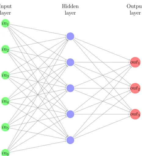
The MLP is a class of feed-forward neural network. It consists of an input layer, a minimum of one hidden layer, and an output layer [9]. A depiction of an MLP is shown in Figure2.2.

Inputs are fed into the network, after which there can be several hidden layers. De-pending on the design chosen, the classes of MLPs can be described as shallow or deep; i.e., an MLP with multiple hidden layers is considered to be relatively deep, whereas an MLP with fewer hidden layers is considered to be relatively shallow.

Each connection between layers has an associated weight with which the input is mul-tiplied. Then, the sum of the weighted inputs enter a node, which usually contains an activation function. The activation function maps the weighted sum of the inputs to an output; this function can be highly non-linear or linear, depending on the application [10]. The activation function can be thought of as a decision function which emits an output (decision) based on given inputs. Examples of an activation function include the sigmoid, tanh, and Gaussian functions. A visual representation of the neuron is shown in Figure 2.3.

(20)

in1 in2 in3 in4 in5 in6 Input layer Hidden layer out1 out2 out3 Output layer

Figure 2.2: A general example of an MLP architecture with 6 inputs, a hidden layer, and 3 output classes

The main purpose of the activation function is to provide a discrimination method for the weighted inputs [10]. A major advantage of MLPs are their ability to discriminate multi-dimensional and non-linear data. As more nodes are added to a MLP, the higher order the decision boundary shall be.

Consider two variables that form the ’half moon’ clusters shown in Figure 2.4. These clusters can represent anything - for illustrative purposes, consider the axes to represent the width of a particular feature vs. the height of a feature. The two different colour clusters can represent two classes of the same object. To find an MLP based decision boundary that will accurately discriminate between the two classes, the number of nodes or layers in the hidden layers will dictate the order of the discrimination boundary.

(21)

x1*w1 x2*w2 Inputs Σ Sum Inputs f Activation function θ Output

Figure 2.3: Diagram of a neuron and activation function

Figure 2.4: The effect of the number of modes in an MLP based decision boundary (from left to right): 1 node in hidden layer, 2 nodes in hidden layer, 3 nodes in hidden layer

The decision boundary for 1 node appears to mis-classify several data points, whereas the highest order decision boundary (3 nodes) does a much better job of separating the two classes. Therefore, the 3 node architecture is most appropriate for classifying the two data classes. This concept is very important to consider for the MLP design.

Mathematically, inputs are fed forward through the MLP, with the output of each node modeled as: o=f( l X i=1 wixi −θ) (2.6)

Where o is the output from the node, x is the input(s) to the node, and w is the weight(s) to the input [9]. For the first iteration of training a MLP, the weights are typically initialized to a small random value [9]. When the output propagates through the MLP, it is compared to the ’true’ value of the output (i.e., the label of the input). To determine how well the MLP is fitting the true output, a loss function is needed to evaluate performance. The subsection 2.4 Training Neural Networks will go into details as to how

(22)

MLP training works.

2.3

Convolutional Neural Networks

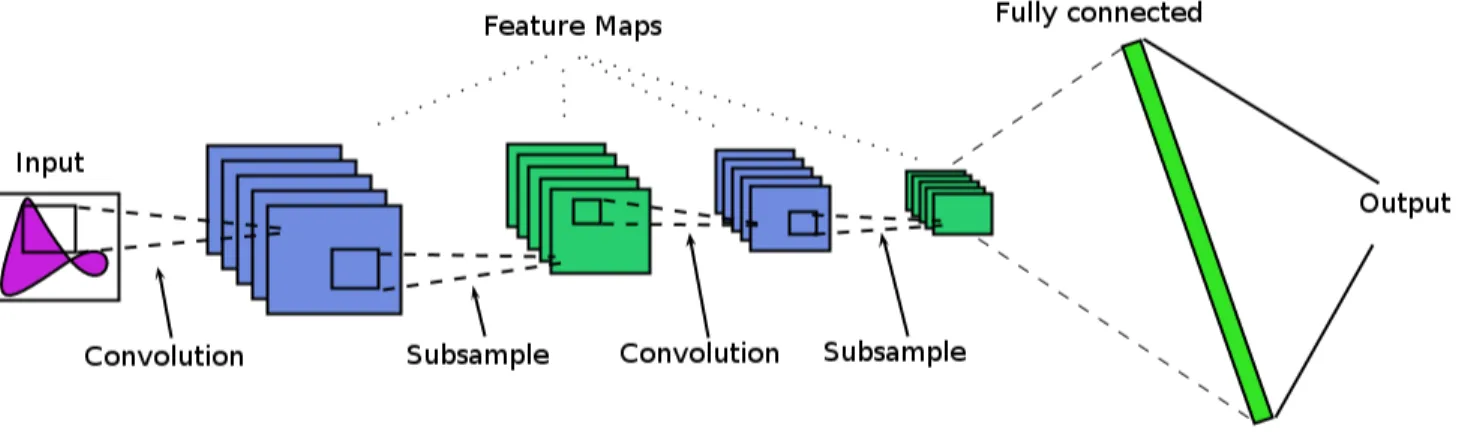
Convolutional neural networks work in similar principle to MLPs in the sense that both architectures are composed of neurons that have learnable weights and biases [11]. The main advantage to CNNs over MLPs is their ability to accept spatial context and multi-dimensional spatial information [11]. CNNs provide the ability to learn features from 2D or 3D images and signals. For the purpose of this thesis, CNNs will be leveraged to add spatial context to the tissue/non-tissue classification problem. This section will provide a brief overview of the CNN framework.

An example of a possible structure of a CNN is represented in Figure 2.6. Consider an example where the input (i.e., a desired set or class of images) has to be learned and classified by an algorithm. To learn features from a set of images, a set of images are fed into a CNN, where a convolution operation is performed by a filter. Mathematically, convolution between two functions over an infinite interval is defined as [10]:

p(z) =p(x)∗p(y) = Z ∞

−∞

p(x)p(z−x)dx (2.7)

In the context of CNNs, the convolution function can be simplified as a dot product between the weights of the filter and the input [11]. To illustrate a simple example, Figure 2.5 shows a convolution operation on two 2x2 matrices.

Figure 2.5: Example of convolution in a 2D context

In practice, the convolution operation by the filter is slid across a padded version of the image in a stride length that depends on the desired output shape of the convolution operation.

CNNs also use sub-sampling to reduce the spatial size of the input, which in turn leads to a reduction in the number of parameters and computation of the network [11]. An

(23)

Figure 2.6: Diagram of a CNN structure where the input image features are learned example of a max pooling operation is shown in Figure 2.7. Here, a 4x4 image block is reduced to a 2x2 block by taking the maximum value (max pooling) of a 2x2 subset of the 4x4 block.

Figure 2.7: Operation of a 2x2 max pooling layer - each 2x2 block of data is reduced by picking the max value

Finally, the sub-sampled inputs can be flattened by re-arranging a 2-dimensional array into a 1-D vector. The 1-D vector is then fully connected to a series of neurons, which are then fed into an activation function; examples of the activation function can include the sigmoid function or a rectified linear unit [12]. The fully connected layer is connected to an output node (or nodes), which classify the image.

(24)

The fully connected layer contains learnable weights, which can be found via optimiza-tion methods (which are discussed in the next subsecoptimiza-tion). The output from the CNN is the resultant classification desired. This concept will be utilized to find tissue vs. non-tissue features in MSI data.

2.4

Training Neural Networks

Training a neural network, whether it is a MLP or CNN, refers to finding the weights of a neuron or filter. Typically, weights are deemed to be most suitable if they minimize a loss function (within the context of the training data). For problems which involve binary classifiers, a common model to measure error (or loss) is known as the Kullback-Leibler divergence (KL). KL divergence quantifies how close a probability distribution, p, is to a candidate distribution, q [13]. The KL divergence can also be referred to as the relative entropy or cross-entropy [13]: DKL(p||q) = X i pilog2 pi qi (2.8)

DKL is defined as non-negative, however it is unbounded and can potentially equal

infinity if there is substantial difference between p and q [13]. DKL can equal 0 if the

probability distributions p and q are equal (i.e., there is no relative entropy between the two distributions) [13].

The KL divergence can be used as a loss function to determine how well the weights of the MLP/CNN are performing relative to the true output where the predicted distribution. With the KL divergence, it is then possible to set-up an optimization problem that aims to minimize the KL divergence, while updating the weights of the MLP. There are several algorithms that can be used to solve optimization problems - for the scope of this thesis, the stochastic gradient descent method (SGD) will be used.

SGD works by finding the best direction to update the weights of the MLP; i.e., find the weight update that will lead to a lower loss [11]. Mathematically, SGD takes the differential of the loss function with respect to the weights to derive an expression [11]. The expression is used to calculate a weight update as shown by the following equations [9]:

∆w=−η∇wDKL (2.9)

(25)

Whereη is the learning rate of the SGD algorithm,∇wDKL is the partial differential of

the loss function (in this case the KL divergence),w represents the weight being updated, and k represents the specific epoch or data set.

The SGD algorithm continues iteratively until a stopping criteria is fulfilled. The cri-teria can include; the loss function dropping below a pre-defined threshold, theδw change

drops below a pre-defined threshold, or the maximum number of iterations has been com-pleted.

An important part of training a neural network is validating the neural network. Typ-ically, data used to train a neural network can be divided into two classes; ’training data’ and ’validation data’. Training data is used to train the neural network (i.e., find the weights), whereas validation data (separate from the training data) is used to test the per-formance of the neural network. When a neural network is trained, loss can be calculated for both the training and validation data set. The loss metrics for both the training and validation data set can also be used as a criteria to halt the training process.

(26)

Chapter 3

State of the Art

Several approaches have been pursued by researchers to characterize skin in colour images, as well as tissue in NIR multispectral images. The approaches can be generalized as statistical based approaches, and artificial neural network based approaches. This chapter will review the literature pertaining to these approaches, and how this thesis will build upon previous works.

3.1

Statistical Approaches

Cha et al. take an optimization approach by creating a probability density map and classify tissue structures based on intensity thresholds [8]. This particular approach utilizes masking layers, as well as Gaussian filters/overlays [8]. This approach appears to segment multispectral images quite well, however it is unclear how well these techniques perform across varying types of tissues (only porcine tissue was tested), and how the algorithm can be generalized to other tissues.

A statistically intensive approach is taken by Deng et al. to characterize healthy vs. cancerous tissue. They characterize the average and standard deviation of calculated met-rics from multispectral images for cancerous and healthy tissues [14]. Then, they perform a t-test to determine if the tissue is cancerous or not [14]. Although effective, this approach suffers from requiring large sets of data (in this case, 450 patients) to characterize and develop a profile.

There are several contemporary techniques for skin classification that are based on characterizing the visible spectrum [15]. One such technique is presented by Jones et al. A

(27)

large dataset is scraped from the Internet which contains images of human skin as well as non-skin items - approximately 1 billion pixels from these images are used to create a skin vs non-skin dataset. By building histograms from each colour channel, the researchers are able to separate the skin vs. non-skin pixels to a classification rate of 80%, with a 8.5% false positive rate [16].

Mendenhall et al. approach skin classification by using both the visible and NIR spec-trum, as many approaches that solely rely on the colour spectrum can have relatively high false-alarm rates (8% to 15%) [17]. The authors utilize information from the spectral ab-sorption of tissue components such as hemoglobin, melanin, and water. By leveraging the absorption profiles across the NIR spectrum, robust classifiers can be developed [17]. The authors capture registered images at multiple wavelengths (227 spectral channels) from 400-2500 nm to characterize tissue vs. non-tissue objects. Given that some of the spec-trum utilized is in the visible range, mixed colour and NIR Gaussian distributions are built. These mixed Gaussians are used to classify pixels into tissue and non-tissue; the authors report an accuracy of 98.6% with a false alarm rate of 1.1% against their test images [17]. However, the authors do state that acquiring such large data sets in real time (227 images per frame) can be extremely expensive. They go on to state that the performance gains may not justify the incurred cost [17].

Another statistical tool that has had some success in multispectral image classification is principal component analysis (PCA) [2]. This technique has been used to evaluate skin chromophores, and to extract blood and melanin data from RGB images[2].

Chao et al. use PCA and multispectral/hyperspectral imaging for the purpose of de-tecting chicken skin tumors. The spectral range used in these experiments was from 420 to 850nm; three bands were selected for further analysis based on the results of PCA from the hyperspectral image set. Images from wavelengths of 465, 575, and 705nm were used to manually label tumorous and normal regions (labeling performed by a trained veteri-narian). Using these labeled data sets, the researchers perform feature engineering and derive various metrics for the labeled regions such as coefficient of variation, skewness, and kurtosis [18]. These features are then used to create classifiers for normal and tumorous tissue by means of fuzzy logic classifiers, and were able to obtain successful classification rates of 91% and 86% for normal and tumorous tissue, respectively [18].

Although leveraging the visible spectrum shows some excellent results, there are some limiting factors. There can be significant overlap between skin and non-skin intensities [15]. Furthermore factors such as ambient lighting and objects that resemble tissue colour can lead to problems with statistical methods that seek to leverage the visible specturm [15].

(28)

3.2

Artificial Neural Network Approaches

There are many accurate and robust approaches to classifying human tissue which include artificial neural networks. This section will discuss some of these works that have been published.

One such approach is presented by Al-Mohair et al., who combine a K-means clustering method with an MLP. Using colour images, they transform the image into a colour space which enhances separability between skin and non-skin pixels (YIQ colour space). After transforming the image, the image is divided into smaller blocks of data, which are then used to create texture descriptions of the skin. These texture descriptions and blocks are used as inputs to an MLP, which discriminates regions of the image into skin/non-skin. Once these regions are identified, a binary mask is created, which is then combined with a K-means clustering process to create a mask for skin/non-skin areas of the image. The authors achieve an accuracy of 87.2% with this technique; using the MLP by itself yields an accuracy of 82.3% [19].

Jolivot et al. propose an MLP approach to classifying melanoma vs. healthy skin cells [3]. They theorize that if given a collection of healthy skin images vs. disease state skin images, they can train an MLP to classify healthy and diseased skin cells. The authors test their theory on a standard 24 colour MacBeth Colour Checker (often used to calibrate colour cameras). They show an excellent ability to predict calibrated colour patches, and state that this technique may be a viable solution for future MSI classification [3].

Carrara et al. successfully employ a NIR MSI regime combined with an MLP design to resolve melanomas. Their study employed a large clinical set of data (2142 patients) which was used for training the MLP. Then, the researchers performed a study that compared the prediction rate of their MLP to that of a trained clinician. The study concluded that the MLP was able to emulate clinician opinion with a sensitivity of 88% and specificity of 80% [4]. The MSI wavelengths the researchers used in this study were from 483-950nm.

Zuo et al. leverage CNNs and recurrent neural networks (RNNs) for skin classification tasks. CNNs assume that all inputs and outputs are independent of each other, whereas the outputs of RNNs depend on previous computations [20]. The authors state that simply using a CNN may not be sufficient to classify skin and non-skin pixels, as CNNs do not take into account the relationship between pixels and their neighbours [20]. Zuo et al. design a neural network which contains a CNN structure with integrated RNN layers. They theorize that the convolutional layers will capture generic local features, and the RNN layers will add further spatial context [20]. On two separate databases of test images, they achieve accuracies of 95.93% and 98.10%.

(29)

Artificial neural network approaches appear to yield promising results for modeling MSI data. These techniques may be effective for the tissue/non-tissue classification problem.

3.3

Next steps

Given the current state of the art, this thesis seeks to build upon the previous research. The results presented by Mendenhall et al. show that leveraging the optical response of tissue at multiple wavelengths can be used to build an extremely accurate classifier. However, their high accuracy may be attributed to using hundreds (227) spectral slices of data, which the authors concede may be cost and computationally prohibitive [17]. Therefore, it is desirable to cut down the number of spectral slices to make this technique viable. However, with fewer features, basic statistical techniques may not create enough separation between tissue and non-tissue pixels as shown by the results presented by Chao et al.

On the other hand, artificial neural networks appear to yield excellent results without the need for hundreds of features/spectral slices. In general, it appears that techniques which account for spatial context such as those presented by Zuo et al. and Al-Mohair et al. appear to yield superior results than MLP based approaches proposed by Jolivot et al. and Carrara et al.

Therefore, artificial neural network based classifiers will be pursued, as the application for this thesis will have limited spectral bands of data to work with (four wavelengths in the NIR region). Both MLP and CNN based approaches will be pursued, and their performance will be compared.

(30)

Chapter 4

Proposed approach

To classify tissue using an MSI system, tissue and non-tissue objects must be characterized across the MSI system spectra. For the context of this thesis, the industrial application is medical imaging with an MSI camera/illumination system at Christie Digital Systems (Kitchener, ON). Images will be collected at Christie Digital Systems, and these images will be the basis of training the algorithms to classify images into tissue/non-tissue.

Given input images to be characterized, two main neural network classes, CNN and MLP, will be designed to characterize tissue and non-tissue data. Both designs will leverage manually labeled data sets captured from the MSI system. In terms of features, the MLP will utilize average pixel level spectra from tissue and non-tissue data as inputs. For the CNN design, 2 dimensional ’patches’ of tissue and non-tissue data will be used as inputs to incorporate spatial context.

The ultimate goal of this work is to train neural network designs to discriminate regions of MSI data that are relevant (i.e., data reduction of non-tissue areas). Therefore, given the output weights/architecture from each design of neural network, MSI data sets will be processed and data reduction will take place by ’masking’ non-tissue areas of the MSI data. The effectiveness of the data reduction will be evaluated both qualitatively and quantitatively.

4.1

Data Collection

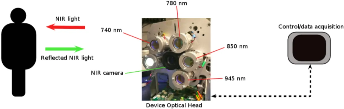
The proposed approach will utilize an imaging system created at Christie Digital Systems. A high level diagram of the imaging system is shown in Figure4.1.

(31)

Figure 4.1: Configuration of the device used for data collection

MSI data (8 bit gray-scale images from the NIR sensor) is captured from four different wavelengths; 740nm, 780nm, 850nm, and 945nm. Each LED is turned on sequentially for 20ms (to minimize any error due to movement). The NIR camera is configured to capture an image during each LED illumination cycle. A ’blank’ image is also captured where no illuminators are active; this image is subtracted from each LED image to compensate for ambient lighting.

An imaging study was conducted at Christie Digital Systems, where forearm image data was captured from subjects of varying age, tissue composition, and skin tone (Fitzpatrick skin types I-VI). Data was captured from 42 subjects; this data was used as labeled ’tissue’ data.

Images of common operating room non-tissue objects were also collected, e.g. sponges, sterile cloths, surgical instruments. These images were used as the labeled non-tissue data. After the data was collected, two distinct approaches for classification were explored. For each approach, features from the MSI data set had to be extracted to create any type of machine learning model. An MLP approach used the pixel-level spectra of tissue/non-tissue data as features to classify regions of MSI image sets. A CNN approach used spatial context in the MSI data to evaluate tissue/non-tissue.

The diagram in Figure 4.2 shows how the data acquired by the MSI system is utilized. Features are extracted from the multispectral images and fed into the MLP or CNN classi-fiers. The output from these classifiers is a ’mask’ that will black out all non-tissue regions in the images, and leave the tissue regions intact.

(32)

Figure 4.2: System data-flow diagram to create the tissue/non-tissue mask

4.2

Design and training of Neural Networks

The two architectures, MLP and CNN, must be designed and trained to identify regions of tissue and non-tissue in MSI data. Hyper-parameter tuning was used to find an appropriate design that will yield the best accuracy on training and validation data.

Once hyper-parameter tuning was done, the ideal architecture was trained for identify-ing tissue and non-tissue. The weights and structure for each design were saved and used to test new MSI data sets for their effectiveness.

All design iterations and research was conducted with open-source Python libraries -Tensorflow[21] and Keras[22]. The Tensorflow package has extensible libraries and data structures for creating neural networks; the Keras package is a simplified and intuitive front-end toTensorflow, and is used to rapidly create prototype neural networks.

4.3

Application of Neural Networks to MSI data

Once the neural networks have been designed and the weights for each learnable parameter were saved, the MLP and CNN architectures were fed a set of test images to find regions of tissue and non-tissue. The test images were new images (i.e., images that were not part of the training process). Each pixel of the MSI data was evaluated for tissue/non-tissue, and all non-tissue areas were masked. The effectiveness of each design was then evaluated both quantitatively and qualitatively.

(33)

Chapter 5

MLP Approach

To design an architecture for an MLP, the number of nodes and layers must be selected such that the MLP produces accurate results. To achieve an optimal design, a hyper-parameter optimization approach was taken to try various architectures to determine the appropriate number of hidden layers and activation nodes. The number of hidden layers and nodes will be systematically altered, and the training/validation loss data will be examined to evaluate the effectiveness of each architecture.

5.1

Single Layer Design

To classify tissue/non-tissue for MSI data, an MLP design is proposed which uses pixel-level spectra as inputs and a single hidden layer with the same corresponding number of nodes; i.e., givenn wavelengths, there will ben number of nodes which will take the pixel-level spectra of each wavelength as an input. There is 1 hidden layer which also contains n nodes. The diagram of the specific MLP architecture created for is shown in Figure 5.1, which is for four wavelengths.

Iλ denotes the average pixel-level spectra at each wavelength. All the connecting lines

represent a weight that relates the input to the hidden layer, and the output of the hidden layer to the output layer. The activation function used for each node is the sigmoid function. The output of the MLP is a decimal number between 0 and 1, which can be used to estimate the presence of tissue in accordance to the labels given to the data (i.e., tissue=1, non-tissue = 0).

(34)

I740 I780 I850 I945 Output Hidden layer Input layer Output layer

Figure 5.1: The architecture of the single layer MLP - Iλ is the input average pixel-level

spectra from each wavelength. All connections between layers and nodes signify weights which are solved for by the back-propagation method. Output of the MLP is a decimal value between 0 and 1 (above or equal to 0.5 =tissue, below 0.5 = non-tissue). Each node signifies the sigmoid activation function

5.2

Training the MLP

Pixel-level spectra were manually sampled, across all wavelengths, from images that had instances of tissue and non-tissue. A 10 pixel by 10 pixel region of interest (ROI) was averaged at each instance of tissue/non-tissue. These pixel-level spectra averages are the inputs to the MLP for building the model.

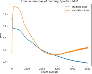
The MLP was trained by using binary cross-entropy as a loss function, and stochastic gradient descent for optimizing the loss function (as outlined in Chapter 2); the training data was split into a training subset and a validation subset of 80% and 20% respectively. The training algorithm was run for 5000 epochs to determine an optimal number of training epochs, i.e., the number of epochs which will yield minimum loss on the training set and validation set.

(35)

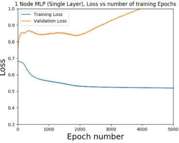
Figure 5.2: MLP training and validation loss vs. number of epochs

The Keras code used to build and train the model is provided in AppendixB. A block diagram is shown in Figure 5.3 which illustrates the overall architecture of the MLP.

After running the training algorithm for 5000 epochs, the optimal number of epochs is found to be 2838 as shown in Figure 5.2. At this number of epochs, the validation set loss reaches a minimum. Although the training data set loss continues to decrease, it is important not to over-fit the data, as continuing the training algorithm causes the validation set loss to rise after epoch number 2838. Training the MLP to 2838 epochs gave a training accuracy of 82.2%.

5.3

Hyper-parameter Optimization - Nodes

The MLP discussed in the previous section was designed by using a process known as hyper-parameter optimization; where neural network hyper-parameters are systematically altered until a desired result is reached. This section will discuss how the hyper-parameter optimization was conducted.

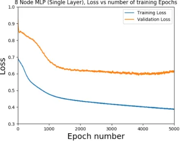
For optimizing the number of nodes to be used in a hidden layer, an initial singular hidden layer will be assumed. This layer will evaluate 1, 2, 4, and 8 node architectures. Training and validation loss graphs will be generated for 5000 epochs as shown in Figures

(36)

Figure 5.3: Block diagram for the MLP design for classifying tissue/non-tissue

5.4 to5.7.

When evaluating the loss functions of each candidate design, the convergence between the loss and training functions are evaluated. It is evident from a qualitative perspective that the single layer 4 node design shown in Figure5.6 shows the best minimization of the training and validation loss at approximately 3000 epochs. Although Figure5.7also shows excellent potential (8 node design), as it appears to have the same approximate training and validation loss profile as the 4 node design. The 4 node design is preferred, as from an implementation point of view, the 4 node design will have a faster run-time.

(37)

Figure 5.4: Loss functions of a single layer MLP design with 1 activation node

(38)

Figure 5.6: Loss functions of a single layer MLP design with 4 activation nodes

(39)

5.4

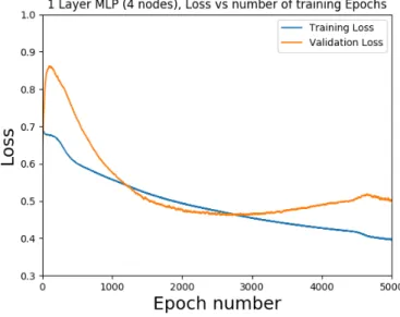
Hyper-parameter Optimization - Layers

Similar to the procedure where the optimal number of nodes was found, the number of layers vs. training and validation loss was explored. Given that the 4 node architecture is preferred, 4 nodes were assumed for this tuning exercise. A single hidden layer will be initially assumed, and layers will be sequentially added. The training and loss functions will be analyzed for each architecture.

(40)

Figure 5.9: Loss functions of 2 layer MLP design with 4 activation nodes

(41)

Figure 5.11: Loss functions of 8 layer MLP design with 4 activation nodes

The training and validation loss profile is lowest for the single hidden layer design. The 2, 4, and 8 layer designs reach a steady state (Figures 5.9 to 5.11), however their loss profiles are much higher than the single hidden layer design loss profile shown in Figure 5.8. Therefore, a single hidden layer design was pursued.

(42)

5.5

MLP Results

Quantitative tests were performed on a ’challenge’ MSI data set of 3 different configu-rations. The configurations have tissue as well as non-tissue objects in the frame. The challenge MSI data set was not part of the training or validation set.

The classification results are shown in Figures 5.12-5.14. The original 780nm image is shown in the left, and the corresponding classified image is shown on the right. Black pixels in the classified image correspond to non-tissue.

Figure 5.12: Test Image 1 for MLP design; (left) 780nm image of MSI data set, (right) resultant classified image

For each classified image, regions of known tissue and non-tissue are labeled manually. With these known regions, the accuracy, sensitivity, and specificity were computed and summarized in Table5.1.

(43)

Table 5.1: Performance metrics of the MLP model against three test images

Test Image Accuracy Sensitivity Specificity

1 0.844 0.882 0.825

2 0.807 0.806 0.807

3 0.865 0.874 0.860

Average 0.839 0.854 0.831

S.D. 0.03 0.04 0.03

The results show that using an MLP with pixel-level spectra as features can be a viable solution to classify tissue. However, this approach fails to generalize tissue and non-tissue areas that have similar pixel-level spectra. For example, Figures 5.12-5.14 show that at edges where there is gradual intensity roll-off, the algorithm mis-classifies these regions as tissue. Furthermore, some areas at the edges of the forearm are mis-classified as non-tissue, when the area is in fact tissue. To improve upon this design, some spatial context must be added to the MLP architecture.

(44)

Chapter 6

CNN Approach

To expand upon the MLP approach, the CNN is designed to integrate spatial context with pixel level spectra. For this particular design, ’patches’ of tissue and non-tissue samples (20 by 20 pixels) were taken from each wavelength image and were labeled as tissue/non-tissue. The CNN was then trained by using binary cross-entropy as a loss function, and stochastic gradient descent was used for optimizing the loss function. The design of the CNN is shown in Figure6.4.

Figure 6.1: MSI set with an example of training ’patch’ selection (20px by 20px) for tissue and non-tissue

(45)

6.1

CNN Design

The structure of the CNN is designed with 2 convolutional layers, each with 5 convolutional filters. The first layer has filters of size 4x4 pixels, and the second layer has 2x2 pixel filters. The type of filter used was initialized with random weights drawn from a uniform distribution in the interval described in the following equation, taken from the techniques presented by Glorot [23]. Wij ∼U[ −1 √ n, 1 √ n] (6.1)

WhereWij represents the weights of the filter at indicesi andj. The parameters within

the brackets represent the interval, where n represents the size of the matrix upon which the filter is being applied, and the operand U refers to a uniform distribution.

As an example, for a singular 4x4 filter, a random uniform distribution for a 20x20 image (i.e. from √−1

20 to 1 √ 20 appears as:     0.0881689 0.0638623 −0.0312524 −0.0984284 −0.2173570 −0.0937632 0.1427977 0.1446408 0.2108532 −0.0058700 0.1497313 −0.0743459 0.1077823 0.1916810 −0.0998226 −0.0721026     (6.2)

To gain some intuition on the structure of the CNN, the first convolutional layer struc-ture is illustrated in Figure 6.2. Here it is shown that the 20x20x4 pixel input is fed into the convolutional layer. The 5 filters have a size of 4x4 pixels. To convolve the input, which has 4 spectral ’slices’ of data, the depth of each filter must be equal to 4, i.e., have dimensions of 4x4x4.

Figure 6.2: Illustration of the first convolutional layer of the CNN design

Each filter convolves the multispectral data set, which has been padded with zeros for the convolutional step. The stride length of the convolution is 1, i.e., the convolution is

(46)

performed on every pixel. Therefore an output feature of 20x20x5 is produced, which will go into the next convolutional layer. The successive convolutional layer also has similar padding and stride length.

After the convolutional layers, a max pooling operation is applied, and the inputs are flattened. Finally, the flattened layer feeds into 100 fully connected neurons which contain a rectified linear unit activation function. The connected neurons then connect to a binary soft-max classifier.

6.2

Training the CNN

The CNN was trained by using binary cross-entropy as a loss function, and stochastic gra-dient descent for optimizing the loss function (as outlined in Chapter2); the training data was split into a training subset and a validation subset of 80% and 20% respectively. The training algorithm was run for 100 epochs to achieve an optimum training and validation accuracy as shown in Figure 6.3. The rationale for selecting the architecture and optimal training epochs is covered in the next section (hyper-parameter optimization).

Figure 6.3: CNN training and validation loss vs. number of epochs

The Keras code used to build and train the model is provided in AppendixD. A block diagram is shown in Figure 6.4 which illustrates the overall architecture of the MLP.

(47)

Figure 6.4: Block diagram for the CNN design for classifying tissue/non-tissue The CNN loss graph shows high variability in the validation loss function, which in-dicates that that some cases are alternating between classifying correctly and incorrectly. However, since the overall magnitude of the loss is relatively low, the minimal training loss is sought at 100 epochs. Training the CNN to 100 epochs gave a training accuracy of 98.9%.

6.3

Hyper-parameter Optimization - Filters

For optimizing the number of filters to be used in the convolutional layer(s), 2 convolu-tional layers were originally assumed. These layers had filters added sequentially, and the

(48)

training/validation loss was evaluated for 200 epochs as shown in Figures 6.5 to6.7.

Figure 6.5: Loss functions of a 2 layer CNN design with 5 convolutional filters

(49)

The least amount of noise and the lowest loss in the validation/training curves is shown in Figure6.5(5 filters). The 10 filter and 20 filter designs do show comparable performance to the 5 filter design, as they are approaching 0 loss in the training set, and they have equivalent steady state validation losses of 0.25. However, there is a slight upward trend in the validation loss profile of the 20 filter design, which may be a sign of overfitting.

Given that the three designs show comparable performance, it is preferred to go with the fewest filters, as there will be less weights to train and the computational overhead will be lower.

6.4

Hyper-parameter Optimization - Layers

Similar to the procedure where the optimal number of filters was found, the number of layers vs. training and validation loss was explored. Given that the 5 filter architecture is preferred, 5 filters were assumed for this tuning exercise. Two layers will be initially assumed, and layers will be sequentially added. The training and loss functions will be analyzed for each architecture and are presented in Figure6.8 to6.10.

(50)

(51)

Given the results, the 2 layer CNN design converges to the most stable and minimal loss functions for the training and loss curves. The 4 and 6 layer designs show erratic profiles, which may be due to over-fitting.

In general, there appears to be more noise in the validation loss profile than the training loss profile in each graph. This is due to two principal reasons. Firstly, the dropout layers in the Keras model will randomly turn off a weight during the training process to reduce over-fitting. This will create an appearance of a smoother training loss profile.

Furthermore, due to the relatively small training data set (90 samples), the validation data set sample size is quite small (20% of the training set). Therefore, the validation loss profile will appear to be relatively ’rougher’ than the training validation loss profile.

(52)

6.5

CNN Results

Quantitative tests were performed on a ’challenge’ MSI data set of 3 different configu-rations. The configurations have tissue as well as non-tissue objects in the frame. The challenge MSI data set was not part of the training or validation set.

The classification results are shown in Figures 6.11-6.13. The original 780nm image is shown in the left, and the corresponding classified image is shown on the right. Black pixels in the classified image correspond to non-tissue.

Figure 6.11: Test Image 1 for CNN design; (left) 780nm image of MSI data set, (right) resultant classified image

Figure 6.12: Test Image 2 for CNN design; (left) 780nm image of MSI data set, (right) resultant classified image

For each classified image, regions of known tissue and non-tissue are labeled manually. With these known regions, the accuracy, sensitivity, and specificity were computed and summarized in Table6.1:

(53)

Table 6.1: Performance metrics of the CNN model against three test images

Test Image Accuracy Sensitivity Specificity

1 0.951 0.938 0.967

2 0.937 0.947 0.947

3 0.960 0.935 0.977

Average 0.952 0.944 0.957

S.D. 0.012 0.005 0.017

The CNN results show that incorporating spatial context with the pixel-level spec-tra helps address the shortcomings that were evident in the MLP approach. The mis-classifications in the CNN approach are less than the MLP, as the CNN approach handles transitions and edges much better than the MLP. Furthermore, the overall classification accuracy, sensitivity, and specificity are improved by incorporating spatial context.

(54)

Chapter 7

Qualitative Evaluation of Designs

Additional images of subjects were taken with the test device in an effort to test the capability of the CNN and MLP designs. This section will qualitatively evaluate the efficacy of each approach (MLP and CNN) on additional test images.

Thus far, only forearms have been evaluated by the MLP and CNN designs. Anatom-ically, forearms will have a different tissue composition (in terms of muscle and fat) than other body parts. This section will examine how well each design performs with body parts that have differing muscle and fat compositions. To test robustness to tissue compo-sition, additional test images were taken on volunteers at Christie Digital Systems to see how well the classifier performs on body parts other than forearms. Various parts of the anatomy were imaged from 3 different subjects to test the performance of the CNN and MLP algorithms.

The test images were processed through the CNN and MLP designs. The resulting classified CNN and MLP images are shown in Figure7.1. From top to bottom, the images are; chest, forearm, upper leg, bicep and back.

The CNN model performs well for all of the cases. The CNN masks foreign objects, tattoos, and drapes/clothing well as shown in Figure 7.2. Also, physiological structures such as veins are not misclassified. Furthermore, the false negative rates are very low when looking at large patches of tissue.

To objectively evaluate the effectiveness of each approach, large ROIs were overlaid on the tissue pixels (i.e., large enough to cover most of the tissue), and the percentage of correct tissue classifications were calculated for each image. The results are shown in Table 7.1.

(55)

Figure 7.1: CNN design classification results on other body parts - Left: original 780nm image. Middle: CNN generated masked image. Right: MLP generated masked image

(56)

Table 7.1: Percentage of correctly classified tissue pixels in ROI - MLP vs CNN MLP CNN Forearm 79.7% 99.8% Chest 36.6% 100% Leg 68.7% 99.4% Bicep 41.3% 100% Back 16.3% 100%

Figure 7.2: Enlarged comparison of CNN and MLP performance on bicep tissue The MLP does not perform as well as the CNN in general - it is notably worse in situations where there is no ’forearm’ data (e.g., bicep, chest, leg, back). Since the MLP relies on pixel-level spectra, and the training data came from forearms, it will be less likely to work on differing body parts that have different pixel-level spectra responses (i.e., areas with different tissue composition than a forearm). An example of the poor performance is evident on the chest image. Figure 7.3 shows an enlargement of the CNN and MLP performance on the chest tissue.

A possible explanation for the poor results by the MLP on other tissue types may be due to the differing optical properties of fat and water, which vary across anatomical sites. To understand specifically why the tissue response is slightly different, the optical prop-erties of lipid and water must be understood, as different body parts may contain varying

(57)

Figure 7.3: Enlarged comparison of CNN and MLP performance on chest tissue amounts of lipid and water. The absorption profile of lipid and water is shown in Figure 7.4 [24] [25] [26].

Since the absorption profiles of lipid and water vary drastically in the 945nm range (where one of the MSI data images is captured), the absorption profiles are likely to be the root cause as to why the MLP fails to correctly classify tissue/non-tissue.

(58)

Figure 7.4: Absorption coefficients of fat and lipid vs wavelength [24] [25] [26]

7.1

Effects of Over-fitting

To test the effect of over-fitting on the masking performance of the CNN, an experiment was done on the set of images shown in the previous chapter. The CNN model was re-trained with its original CNN design, and a 2 layer, 20 filter CNN design which was re-trained. The intent of the 2 layer, 20 filter design is to create a model that has been over-fit.

The bicep image in particular highlights the consequence of using an over-fit model. Comparative results are shown in Figure7.5.

Using 20 filters to characterize and classify tissue (vs. using 5 filters) can lead to characterizing features which may be either irrelevant and/or redundant. Selecting the appropriate number of convolutional filters is critical when designing a CNN.

(59)

Figure 7.5: The effect of over-fitting CNN design - top: 5 filter CNN design, bottom: 20 filter CNN design, left: original 780nm image, right: masked image

(60)

Chapter 8

Future work and Conclusion

8.1

Summary of Contributions

To summarize, the main contributions of this thesis were as follows:

• MLP design that uses pixel level spectra from MSI data to classify tissue and non-tissue

• CNN design that uses spatial context from MSI data to classify tissue and non-tissue • Hyper-parameter optimization for the design of the MLP and CNN models

• Qualitative and quantitative evaluation of the MLP and CNNs on MSI data

8.2

Future Work

To build upon the work shown in this thesis, there are many potential research projects that can be pursued. This section will discuss some potential research avenues and their impact.

8.2.1

Classification of Tissues

Future research can specifically investigate the use of CNNs and MSI data to classify and model specific tissue characteristics, structures, and pathologies.

(61)

In terms of data collection, labeled data sets should be used to train a classifier - for example, if evaluating cancerous vs. healthy tissue, an expert should classify regions of the image that are definitively cancerous or healthy. Crowd sourcing diagnoses and opinions from an expert panel is also a practical method of gathering labels for data.

For longer term future work, unsupervised deep learning approaches should be explored once a large data-set of medical opinion on MSI data sets has been gathered. Unsupervised deep learning algorithms could find commonality between various classifications of tissue and enable more meaningful insights to medical MSI data.

8.2.2

Model Fitting

From a non-classification standpoint, it would be interesting to investigate whether an MLP/CNN architecture could be used to assist with analyte concentration determination. For example, if a system was developed to calculate the concentration of an analyte of interest, and given:

• MSI data-set from candidate system • Set of corresponding extinction coefficients

• ’Gold standard’ data; i.e., known analyte concentration of interest determined by a generally accepted lab method

It would be possible to develop a correction factor by creating a neural network ar-chitecture that would fit a mathematical model to the ’gold standard’. In mathematical terms, consider matrix A as a matrix of observations, x as the model coefficients (i.e., extinction coefficients), andb as the final calculated value of the concentration of interest:

A=bx (8.1)

Ax−1 =b (8.2)

Then, consider a correction factor that is a function of the difference between the calculated value and the ’gold standard’ value from another method:

(62)

Using a neural network architecture, denoted by the functionNN, and MSI observations A, a correction factor can be modeled as:

k =N N(A,∆) (8.4)

Finally, the correction can be implemented as:

A[1−k]x−1 =b (8.5)

This example, although simplistic, is the general framework for how future research can be conducted on finding tissue analyte concentrations with MSI data sets.

8.2.3

Ensemble Methods

For real-time applications research, the MLP approach is attractive due to its relative speed of implementation. The MLP approach can still be a viable option if given a diverse enough data-set. As shown in the qualitative analysis, differing body compositions will yield different magnitudes of pixel-level spectra.

Therefore, a study must be organized that samples several types of body tissue to build a more robust classifier. Also, the MLP can be used in conjunction with other methods such as random forests and support vector machines (SVMs) to get better accuracy.

A separate study can quantify the speed of implementation of each model on a stan-dardized data set. Furthermore, the trade-off between speed and accuracy for different models and algorithms can be investigated.

8.3

Conclusion

This thesis demonstrated two distinct approaches and designs for classifying MSI tissue data - a multi-layer perceptron, and a convolutional neural network design.

It was found that the CNN design yields excellent reliability and accuracy compared to the MLP. The accuracy, sensitivity, and specificity of the CNN is 95.2, 94.4, and 95.7% as measured on a test set of MSI data. The MLP results on the same data set for accuracy, sensitivity, and specificity are 83.9, 85.4, and 83.1% respectively. It is also demonstrated that the CNN design shows superior robustness to tissue types and body composition.

(63)

The MLP is considered due to its relative simplicity and speed of real-time implemen-tation, however it does suffer from poor generalization and selectivity. It was found that the MLP design is highly dependent on the tissue composition of the training set, and fails to generalize to other body parts. Furthermore, the MLP fails at sharp contrast transi-tions (such as borders, veins). Conversely, the CNN design was robust to different tissue compositions, and generalized well to other body parts.

There are several paths for future work to take place. Using the designs and methods shown in this thesis, further MSI studies can be conducted in the context of diagnostic applications which require tissue classification. Furthermore, other fields which utilize MSI data can leverage the same techniques for classification tasks; e.g., remote sensing tasks or geospatial analysis.

This thesis has given an introductory glance at the potential of combining neural net-work architecture and tissue optics. This author hopes that this thesis has laid the ground-work for future research in classification of tissues, and that clinically useful classifiers are designed from the techniques presented.

(64)

References

[1] Guolan Lu and Baowei Fei. Medical Hyperspectral Imaging: A Review. Journal of Biomedical Optics, 19(1):010901, Jan 2014.

[2] Jana M Kainerstorfer, Paul D Smith, and Amir H Gandjbakhche. Noncontact Wide-Field Multispectral Imaging for Tissue Characterization. IEEE JOURNAL OF SE-LECTED TOPICS IN QUANTUM ELECTRONICS, 18(4), 2012.

[3] Romuald Jolivot. Reconstruction of hyperspectral cutaneous data from an artificial neural network-based multispectral imaging system. Computerized Medical Imaging and Graphics, 35(2), Mar 2011.

[4] M Carrara, A Bono, C Bartoli, A Colombo, M Lualdi, D Moglia, N Santoro, E Tolomio, S Tomatis, G Tragni, M Santinami, and R Marchesini. Multispectral imaging and artificial neural network: mimicking the management decision of the clinician facing pigmented skin lesions. Physics in Medicine and Biology, 52(9):2599– 2613, May 2007.

[5] Christopher D Malon and Eric Cosatto. Classification of mitotic figures with convo-lutional neural networks and seeded blob features. Journal of Pathology Informatics, 4, 2013.

[6] Shadi Albarqouni, Christoph Baur, Felix Achilles, Vasileios Belagiannis, Stefanie Demirci, and Nassir Navab. Aggnet: Deep learning from crowds for mitosis de-tection in breast cancer histology images. IEEE Transactions on Medical Imaging, 35(5):1313–1321, 2016.

[7] Steven Jacques. Optical properties of biological tissues: a review. Phys. Med. Biol, 58, 2013.

(65)

[8] Jaepyeong Cha, Azad Shademan, Hanh N. D. Le, Ryan Decker, Peter C. W. Kim, Jin U. Kang, and Axel Krieger. Multispectral tissue characterization for intestinal anastomosis optimization. Journal of Biomedical Optics, 20(10):106001, Oct 2015. [9] Fakhri Karray and Clarence De Silva. Soft Computing and Tools of Intelligent Systems

Design: Theory and Applications. Pearson Addison Wesley, 2004.

[10] Richard O. Duda, Peter E. Hart, and David G. Stork. Pattern Classification. Wiley, 2001.

[11] Andrej Karpathy. Cs231n: Convolutional neural networks for visual recognition. Neu-ral Networks, 1, 2016.

[12] Alfredo Cuesta-Infante, Francisco J Garc´ıa, Juan J Pantrigo, and Antonio S Mon-temayor. Pedestrian detection with lenet-like convolutional networks. Neural Com-puting and Applications, pages 1–7, 2017.

[13] Jonathon Shlens. Notes on kullback-leibler divergence and likelihood. arXiv preprint arXiv:1404.2000, 2014.

[14] Bin Deng, Maxim Fradkin, Jean-Michel Rouet, Mats Lundqvist, Richard H Moore, Daniel B Kopans, Qianqian Fang, and David A Boas. Characterizing breast lesions through robust multimodal data fusion using independent diffuse optical and x-ray breast