New methods for branch-and-bound algorithms

(1)

c

(2)

NEW METHODS FOR BRANCH-AND-BOUND ALGORITHMS

BY

DAVID ROBERT MORRISON

DISSERTATION

Submitted in partial fulfillment of the requirements

for the degree of Doctor of Philosophy in Computer Science

in the Graduate College of the

University of Illinois at Urbana-Champaign, 2014

Urbana, Illinois

Doctoral Committee:

Professor Sheldon H. Jacobson, Chair

Professor Edward C. Sewell, Southern Illinois University, Edwardsville

Assistant Professor P. Brighten Godfrey

(3)

Abstract

Branch-and-bound (B&B) algorithms, and extensions such as branch-and-price (B&P) are powerful tools for optimization. These algorithms are used in a wide variety of settings, and thus it is beneficial to develop new techniques to improve the performance of B&B algorithms that are independent of the specific problem being studied. This dissertation describes three such techniques.

First, new results for thecyclic best-first search(CBFS) strategy are presented. This strategy groups subproblems into a list ofcontourswhich it repeatedly cycles through. The strategy selects one subproblem to explore from each contour on every pass through the list. Theoretical results are proven showing the gener-ality of the CBFS strategy, and bounds are given on the number of subproblems the strategy explores. More-over, an analysis of various contour definitions is performed to ascertain the factors that drive its performance. In addition, two general-purpose methods are described for B&P algorithms that enable standard integer branching rules to be used while limiting the computation time required to solve the constrained pricing problem (i.e., the pricing problem which respects the branching decisions at the current subproblem). The first method uses a data structure called azero-suppressed binary decision diagram (ZDD) to solve the pricing problem and keep track of previous branching decisions. Bounds are proved on the size of a ZDD for the maximum-weight maximal independent set problem, which is used to solve the pricing problem in a B&P algorithm for the graph coloring problem.

The last method described in this dissertation restructures the search tree in a B&P setting using a wide branching strategy so as to minimize the number of times the constrained pricing problem must be solved. This restructuring is motivated by the Wide Branching Theorem, which guarantees the existence of a smallest search tree for a fixed set of pruning rules. Adelayed branching technique is described that limits the branching factor of the search tree, and forgetful branching is applied to further reduce the number of times the constrained pricing problem needs to be solved in the tree.

Computational results are presented for all methods on various optimization problems (mixed integer programming, graph coloring, the generalized assignment problem, and the simple assembly line balancing problem). Finally, future research directions are presented.

(4)

(5)

Acknowledgments

The trouble with writing acknowledgments is twofold: there’s never enough space to acknowledge everyone who ought to be acknowledged, and they’re rarely very interesting to read unless you’re one of the people being acknowledged. Nevertheless, the work of obtaining my doctoral degree would literally1 _{be impossible} without the endless support of many people, and so I shall endeavor to acknowledge as many of you as possible while at the same time providing some enjoyment for those of you who didn’t make the cut. If your name isn’t here, and you think it ought to be, the next time I see you I’ll give you a pen and let you scribble it in the margins.

I have to start with my family: to my wife Karen, thanks for everything—for rejoicing with me when things were good, for encouraging me when they weren’t, and for telling me to put on my big boy britches when I was being needlessly melodramatic. To Mom, thanks for setting my foundation. I made it this far because of what you taught me, even if I fought you tooth and nail sometimes. To Daddy, thanks for teaching me to never give up and how to think for myself; these are basically required skills for doing research of any kind. To my father-in-law Bob, thank you for your encouragement, and for sparking my interest in OR; I miss you. And to Barbara, thank you for your support and and love, and for lots of entertaining board games. For the rest of my family: thank you for teaching me how to have fun, for teaching me how to laugh (and for laughing at all of my hilarious jokes), and for teaching me how to love. But most of all, thanks for all the margaritas—I never would have made it this far without those.

I also want to express my gratitude to all of the teachers and mentors who have guided me on my educational journey, but two people stand above the rest. Firstly is my advisor, Dr. Sheldon Jacobson. Thank you for providing guidance when I needed it, but also for giving me the space to make mistakes and learn from them. Thank you also for helping to mature my writing abilities. Your feedback on papers is always beneficial and insightful. I look forward to our future relationship, both professionally and personally. Secondly is my undergraduate advisor, Dr. Susan Martonosi (I even spelled it right!): your constant insistence that I should pursue my PhD is the only reason I even considered this path, but it was definitely the right

(6)

path to take. Thank you for your continuing support and mentorship, and for all those bleary-eyed meetings that were too early in the morning for either of us. Let’s not do those again.

To the rest of my doctoral committee, Dr. Edward Sewell, Dr. Brighten Godfrey, and Dr. David Forsyth, thank you for your time and support. Without your many good suggestions and advice, the research presented in this dissertation would be woefully incomplete.

To my academic siblings: Golsheed Baharian, Banafsheh Behzad, Arash Khatibi, Doug King, Estelle Kone, Alex Nikolaev, Laura McLay, J.D. Robbins, and Jason Sauppe, thank you for your long conversations about research, your long conversations about life, and all our group dinners. I look forward to many future collaborative endeavors. When I start my new journal entitledFacts, you can all be in the first issue.

Finally, I’d like to briefly mention the friends who have helped me along this journey. It is quite a long list: Nathan and Audrey, Jason and Colleen, Ben and Jen, Trevis and Jacinda, Scott and Lindsay, Matt and Anna, Mike and Lynn, Ben and Moriah, Peter and Kathryn, Mike and Meredith, Joe and Mel, Jacob and Sarah—and there are many others, as well. There’s some space in the margins for you to add your name if I forgot it. I love you all!

I’d like to offer a special thank you to a place that’s near and dear to my heart: the Midwest. When I first moved there, I hated it, but in the last five years, it has grown on me quite a bit. Now, if only it had less snow in the winters, less humidity in the summers, and more mountains and oceans all year round, I think I would like living there just fine. So long, and thanks for all the fish!

Gloria Patri, et Filio, et Spiritui Sancto. Sicut erat in principio,

et nunc, et semper, et in sæcula sæculorum.

Amen.

Kyrie eleison.

The computational results reported were obtained using the Simulation and Optimization Laboratory at UIUC. This research has been supported in part by the Air Force Office of Scientific Research (FA9550-10-1-0387), the Department of Defense (DoD) through the National Defense Science & Engineering Graduate Fellowship (NDSEG) Program, and the National Science Foundation Graduate Research Fellowship program under Grant Number DGE-1144245. Any opinion, findings, and conclusions or recommendations expressed in this material are those of the author and do not necessarily reflect the views of the United States Government.

(7)

List of Notation

ai An element of the constraint matrixA

A Constraint matrix for an integer programming problem

A An arbitrary search strategy for a branch-and-bound algorithm b Constraint bounds for an integer programming problem β A numerical constant

c A vector of cost coefficients

C A combinatorial set representing a column (or variable) in a column generation scheme ¯

C A subset of a column (or variable) in a column generation scheme

C (C0₎ _{The (restricted) set of columns in a column generation scheme}

d The maximum depth of a search treeT d(_·) The degree function for vertices in a graphG

D A directed graph

D+ _{The transitive closure of a directed graph}_D δ−₍

·) The indegree function (number of incoming arcs to a vertex in a directed graphD) ∆j A bound on the size of the subtree rooted at thejthchild of the current subproblem

∆(G) The degree of the largest-degree vertex in an undirected graph E The set of edges for a graph

E An ordered set of objects or elements (e1, e2, . . . , en)

f The objective function for an optimization problem Fi TheithFibonacci number

φ(y1, y2, . . . , yn) A boolean formula on the variablesy1, y2, . . . , yn

ϕ (1 +√5)/2 Φ∗

j (Φj) The set of (direct) successors of a taskj

G An undirected graph with vertex setV and edge set E G[U] The induced subgraph ofGwith respect to a set of verticesU

(9)

Γi( ¯C) The set ¯C∩ {v1, v2, . . . , vi−1} for an independent set ¯C in a graphG i, j, k Generic indices

Im The idle time for a machinemin a scheduling problem

I A set of indices of non-empty contours for a CBFS strategy J A set of jobs or tasks in a scheduling or assignment problem Ki Theithcontour in a CBFS strategy

K The set of contours for a CBFS strategy

supp(K) The support of the set of contours K, i.e., the set of non-empty contours inK over the course of the algorithm.

κ(·) The contour labeling function for the CBFS strategy

`i(ZC) The set of nodes ofZC which satisfy var(z) =i; theithlevel ofZC

Lz (Lz) The (reduced) eligibility set for a nodezin the maximal independent set ZDD; that is, the

set of vertices available for use (used by at least one valid path) atz λ Lagrange multiplier vector in an integer programming problem M A bound on the length of time needed to explore a subproblem µ(_·) The measure-of-best function for BFS and CBFS

n, m The number of elements or variables in a problem or set [n] The set_{1,2, . . . , n_}

N(U) The set of vertices in a graphGadjacent to vertices inU N[U] The closed neighbor set ofU in a graph G, that is,N(U)∪U

P A path in a ZDD or in a graph

P An optimization problem defined over a search spaceX with objective functionf (π1, π2, . . . , πn) A set of weights (or prices) in a column generation scheme

π(C) P

i∈Cπi; ifC is a singleton, sometimes the set notation is dropped

Π∗

j (Πj) The set of (direct) predecessors of a taskj

q A vector of auxiliary variables for a mixed integer programming problem r The branching factor of the search treeT

R A list of restricted elements, or a tabu list

S A subset of the search spaceX; a subproblem inT

S A set of unexplored subproblems in a branch-and-bound algorithm σi The set of jobs assigned to theithworker in an assembly line problem

t A vector of job or processing times for a scheduling/assignment problem T The search tree built up by a branch-and-bound algorithm

(10)

τz The totally dominated set of vertices at a node z in the maximal independent set ZDD;

that is, the set of vertices dominated by all valid paths fromz u, v Vertices in an undirected graph

u_↔v (u_6↔v) Vertices uandv are (non-)adjacent. U A subset of vertices in a graph

V The set of vertices for an undirected graph wi(Z_C) The width of theithlevel ofZ_C

x An element of the search spaceX; a feasible solution to an optimization problem ˆ

x(ˆx0₎ _{The current (candidate) incumbent solution for a branch-and-bound algorithm}

x∗ _{An optimal solution to an optimization problem}

X A set of feasible solutions to an optimization problem; the search space

ξ The capacity or cycle time for a machine in an assembly line or assignment problem y A vector of variables for a mixed integer programming problem

z A node in a ZDDZ zroot The root node of a ZDDZ

z_`C¯ Denotes that az-to-1path in a ZDDZ_C corresponds to a subset ¯Cof some column inC; i.e.,z yields ¯C.

Z, ZC A zero-suppressed binary decision diagram; a ZDD characterizing the family of setsC

χ The chromatic number of a graphG

|ZC| The total number of nodes and edges in the ZDDZC

1C(·) The indicator or characteristic function for a setC

1,0 The “true” and “false” (or “accept” and “reject”) nodes of a ZDD 2Y _{The power set of a set}_Y

(11)

Chapter 1

Introduction

Thebranch-and-bound (B&B) framework is a fundamental and widely-used methodology for producing exact solutions to NP-hard optimization problems. The technique, which was first proposed by Land and Doig (1960), is often referred to as an algorithm; however, it is perhaps more appropriate to say that B&B encapsulates a family of algorithms that all share a common core solution procedure. This procedure implicitly enumerates all possible solutions to the problem under consideration, by storing partial solutions calledsubproblemsin a tree structure. Unexplored nodes in the tree generate children by partitioning the solution space into smaller regions that can be solved recursively (i.e., branching), and rules are used to prune off regions of the search space that are provably suboptimal (i.e.,bounding). Once the entire tree has been explored, the best solution found in the search is returned. A early overview of the core B&B algorithm was provided by Lawler and Wood (1966); the solution procedure is also covered in the excellent texts by Nemhauser and Wolsey (1988), Bertsimas and Tsitsiklis (1997), and Papadimitriou and Steiglitz (1998).

One reason for the popularity of B&B methods is due to the generality of the solution procedure: B&B-based algorithms can be used to solve many different types of optimization problems in areas of practical interest, including scheduling problems (e.g., airline crew scheduling (Barnhart et al., 2003), sports scheduling (Easton et al., 2003), hospital staff scheduling (Beli¨en and Demeulemeester, 2008; Gendreau et al., 2007)), graph problems (e.g., coloring problems (Mehrotra and Trick, 1996), partitioning problems (Clausen, 1999), clustering problems (Fukunaga and Narendra, 1975)), network design and network flow (e.g., facility location (G¨ortz and Klose, 2012), vehicle routing (Fukasawa et al., 2006), multicommodity flow (Barnhart et al., 2000)), and many others. B&B algorithms are also applied to problems of theoretical importance, including mixed integer programming (Nemhauser and Wolsey, 1988) and non-linear programming (Tawarmalani and Sahinidis, 2004).

An additional reason for the success of B&B-based approaches is due to the simplicity of the method. B&B is easy to explain and implement; moreover, it is easily extensible. This fact allows lessons learned in one problem domain to be easily transferred to other settings. Its simplicity also ensures that mistakes in the algorithm or implementation are less common and easier to detect.

(12)

Many problem-specific enhancements to B&B methods have been developed that have resulted in dra-matic improvements in computation time and solution quality. While problem-specific algorithmic enhance-ments are in many cases critical to the success of a B&B algorithm, new general-purpose enhanceenhance-ments to the framework can yield similar performance gains in many settings at once. Therefore, this dissertation proposes three new general-purpose enhancements for B&B algorithms that can be applied to a wide class of problems while maintaining the simplicity of the approach.

Chapter 3 describes the first of these extensions, calledcyclic best-first search(CBFS). This extension is a new search strategy that can be used with B&B which attempts to balance the diversification and intensification properties of the search process more effectively than other standard search strategies such as depth-first search (DFS) and best-first search (BFS). The eponymous characteristic of the CBFS strategy is its cycling behavior: CBFS groups subproblems together into sets calledcontours, and repeatedly cycles through these contours, selecting one subproblem from each contour to explore on each pass through the search tree. By constructing the contours appropriately, the search strategy can delay exploration of some subproblems and encourage exploration of others, similarly to the way a tabu list operates in local search algorithms. This strategy provides algorithm designers with greater control over how subproblems are explored, and can lead to significant improvements in performance in some settings.

The remaining two extensions described in this dissertation are applied in the context of branch-and-price (B&P); B&P is an extension of B&B which operates in a setting where the number of branching variables is exponential in the input size of the problem. The entire set of branching variables cannot in general be stored in available memory; thus, only a subset of the branching variables is stored at any given time. B&P algorithms combine a conventional B&B search over this restricted pool of variables together with an auxiliary problem referred to as the pricing problem, which is used to introduce new variables into the pool as necessary.

Problem formulations with an exponential number of decision variables are often used to improve the value of the lower bounds used to prune in the search process, as well as to break symmetry that may be present in simpler formulations. However, the pricing problem (which needs to be solved exactly at least once at every subproblem in the search tree) is usually NP-hard as well. Thus B&P algorithms need to balance the computational savings gained by better pruning with the increased computation time needed to repeatedly solve the pricing problem.

A secondary challenge that arises when solving an exponentially-sized formulation with B&P is the necessity of the pricing problem to respect previous branching decisions. In particular, when the pricing problem is solved to introduce new variables into the variable pool, the produced variables must not violate

(13)

any of the branching decisions at the current subproblem. However, communicating these branching decisions to the pricing problem generally significantly increases the difficulty of finding a solution, which in turn increases the overall computation time. The pricing problem with additional side constraints reflecting the branching decisions at the current subproblem is called theconstrained pricing problem.

A final complication due to the large number of variables present in B&P settings is that the resulting search trees are often extremely unbalanced. If the algorithm gets unlucky, it may spend much computation time exploring the deeper regions of the search tree before finding optimal or near-optimal solutions, when instead it could have found an optimal solution much more quickly if it had explored the shallower side of the tree first. For example, given a binary mixed integer programming problem with a large number of covering constraints (of the formP

aiyi ≥b), a single branching decision setting yi = 1 may satisfy a large number

of constraints simultaneously, whereas a branching decision setting yi = 0 may not change the structure of

the IP very much. Thus, a comparatively small number of the former type of assignments will be performed before either a feasible solution is found or the path is pruned. On the other hand, a large number of the latter type of assignments will need to be made before the corresponding path can be pruned.

Chapter 4 presents an extension to B&P algorithms that attempts to address these issues. This extension uses a data structure called azero-suppressed binary decision diagram(ZDD) to encode solutions to the pricing problem; this data structure requires some additional up-front computation time, but then can be queried and updated efficiently to solve the constrained pricing problem as the search progresses. The use of this data structure enables bounds to be computed more quickly in a B&P context, and thus pruning to occur more quickly. This extension also uses the CBFS strategy to counteract the effects of an unbalanced search tree.

A second B&P extension, calledwide branching, is presented in Chapter 5. Instead of trying to improve the solution times of the pricing problem, this extension instead modifies the the branching strategy used by the algorithm so as to limit the number of times the constrained pricing problem must be solved, using an operation called path compression. The path compression operation collapses long chains in the search tree into a single subproblem, and forgetful branching is applied to remove branching constraints that conflict with the pricing problem. Adelayed branchingtechnique is applied to limit the branching factor of the search tree. This new branching strategy has the added benefit of restructuring the search tree so that it is not as unbalanced.

(14)

Chapter 2

The Branch-and-Bound Algorithm

At the most general level, a branch-and-bound algorithm is used to solve some optimization problemP = (X, f), where X (called thesearch space) is a finite set of valid solutions to the problem, and f :X _→R

is the objective function. The algorithm’s goal is to find an optimal solution x∗

∈ arg minx∈Xf(x).

To solve P, B&B iteratively builds a search tree T of subproblems, that is, subsets of the search space. Additionally, a feasible solution ˆx _∈X (called the incumbent solution) is maintained. At each iteration, the algorithm selects a new subproblem to explore from a list S of unexplored subproblems; if a solution ˆx0 _∈_S _{(called a} _{candidate incumbent) can be found with a better objective value than ˆ}_x

(i.e., f(ˆx0₎ _{< f}_(ˆ_{x)), the incumbent solution is updated. On the other hand, if it can be proven that no}

solution inShas a better objective value than ˆx(i.e., ∀x∈S, f(x)≥f(ˆx)), the subproblem ispruned(or fathomed), and the subproblem isterminal. Otherwise, child subproblems are generated by partitioning S into an exhaustive (but not necessarily mutually exclusive) set of subproblemsS1, S2, . . . , Sr, which are

then inserted into T. Once no unexplored subproblems remain, the best incumbent solution is returned; since subproblems are only fathomed if they contain no solution better than ˆx, the solution returned by the algorithm must bex∗

≡x. Pseudocode for the generic B&B procedure is given in Algorithm 2.1.ˆ Algorithm 2.1:Branch-and-Bound(X, f)

1 SetS ={X}and initialize ˆx 2 while S 6=_∅:

3 Select a subproblemS∈S to explore

4 if a solution ˆx0∈ {x∈S |f(x)< f(ˆx)}can be found: Set ˆx= ˆx0 5 if S cannot be pruned:

6 PartitionS intoS₁, S₂, . . . , Sr

7 InsertS1, S2, . . . , Srinto S

8 RemoveS fromS 9 Return ˆx

With respect to this pseudocode, the search strategy affects the order in which nodes are selected for exploration in Line 3 of Algorithm 2.1; the branching strategy affects the way the subproblem is partitioned and the number of produced children (Line 6, Algorithm 2.1); and the pruning rules used in Line 5 of

(15)

Algorithm 2.1 determine whether or notS can be fathomed. Usually, an initial incumbent solution is found (Line 1, Algorithm 2.1) via a heuristic procedure (see, for example, Malaguti et al., 2011).

Note that the set X (and all subproblems) is generally given implicitly; that is, given an element x, membership in a particular subproblem can be checked efficiently, and a partition of any subproblem can be computed efficiently without knowing all the members of X. Then, the complexity of B&B algorithms is related to two factors: the branching factor r of the tree, which is the maximum number of children generated at any node in the tree, and thedepthdof the tree, which is the longest path from the root ofT to a leaf. Thus, any B&B algorithm operates inO(M rd_{) worst-case running time, where}_M _{is a bound on}

the length of time needed to explore a subproblem; however, the presence of pruning rules can substantially improve the algorithm performance.

2.1

Relationships Between Algorithm Components

There are two important phases of any B&B algorithm: the first is thesearchphase, in which the algorithm has not yet found an optimal solutionx∗_{. The second is the}_verification _{phase, in which the incumbent}

solution is optimal, but there are still unexplored subproblems in the tree that cannot be pruned. Note that an incumbent solution cannot be proven optimal until no unexplored subproblems remain; also note that the delineation between the search phase and the verification phase is unknown until the algorithm terminates. In a slight abuse of terminology, a problemP is said to besolvedif the B&B algorithm has completed the verification phase. In this case, the algorithm is said to have produced acertificate of optimality.

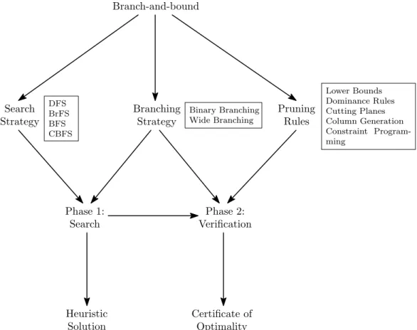
The three algorithmic components (search strategy, branching strategy, and pruning rules) each play a distinct role in B&B algorithms with respect to these two phases of operation (see Figure 2.1). In particular, the choice of search strategy primarily impacts the search phase. To see this, suppose the pruning rules and branching strategy are fixed, and only depend on the value of the incumbent solution (e.g., they compare a subproblem’s lower bound to the incumbent value). In this setting, any search strategy must explore the same remaining set of subproblems once an optimal solution is found.

Moreover, observe that the choice of pruning rules primarily impacts the verification phase, since pruning rules are often relatively weak before an optimal (or near-optimal) solution is known (using the above example, if the incumbent solution has a poor objective value early in the search process the lower bounds will not be able to prune effectively, even if they are very tight). However, the choice of branching strategy has significant impacts on both the search phase and the verification phase: by branching appropriately at subproblems, the strategy can guide the algorithm towards optimal solutions, and limiting the branching

(16)

Branch-and-bound Pruning Rules Branching Strategy Search Strategy Phase 1: Search Phase 2: Verification Heuristic Solution Certificate of Optimality Binary Branching Wide Branching DFS BrFS BFS CBFS Lower Bounds Dominance Rules Cutting Planes Column Generation Constraint Program-ming

Figure 2.1: A diagram of the three main B&B components. The search strategy and the pruning rules pri-marily impact the search phase and verification phase, respectively, whereas the branching strategy impacts both.

decisions made during verification prevents unnecessary work from being performed to produce a certificate of optimality.

There are two important reasons to improve performance of the B&B algorithm during the search phase. First, if the algorithm terminates before producing a certificate of optimality, the incumbent solution can still be returned as a heuristic solution, which may be sufficient in some problems. An example of this behavior can be seen in Fischetti and Lodi (2003), which introduces new constraints in a mixed integer programming framework to attempt to reach a feasible solution quickly.

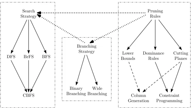
Secondly, finding an optimal solution earlier in the search phase has a direct impact on the size of the search tree (and thus the time necessary to verify optimality), since no further nodes with bounds greater than the optimum value need be explored. Intuitively, this is the rationale behind the result of Dechter and Pearl (1985) showing that best-first search explores the fewest number of subproblems of any search strategy. Figure 2.2 shows the internal relationships between the different types of pruning rules, branching strate-gies, and search strategies. In this figure, solid lines indicate a generalization relationship. For instance, as

(17)

Pruning Rules Lower Bounds Dominance Rules Cutting Planes Column Generation Constraint Programming Binary Branching Wide Branching DFS BrFS BFS CBFS Search Strategy Branching Strategy

Figure 2.2: A diagram of relationships between various B&B algorithm components.

discussed in Section 2.4.4, many constraint programming techniques generalize cutting planes and dominance relations. Furthermore, the CBFS search strategy is a generalization of DFS, BrFS, and BFS (see Chapter 3). Column generation techniques, while not strictly a generalization of other techniques, are closely connected to lower bounding and cutting plane techniques (in essence, column generation adds cutting planes to the dual optimization problem to improve the computed lower bound); B&P algorithms combine a B&B search with column generation (see Section 2.5).

Figure 2.2 also shows the relationships between the pruning rules, the branching strategy, and the search strategy used by an algorithm. In particular, the choice of pruning rules often impacts or limits the choices that can be made in the other two areas. For example, as discussed in Section 2.5, if column generation is used to improve lower bounds, the choice of branching strategies that can be used is limited. Moreover, if dominance relations are used, this may cause BrFS to become a desirable search strategy, since it has the property of never exploring a dominated subproblem. Finally, the choice of branching strategy can itself impact the choice of search strategy. For instance, if the branching strategy chosen produces a particularly unbalanced tree, the CBFS strategy can balance the search process, or variants of DFS can limit the depth explored at any stage in the algorithm.

(18)

2.2

Search Strategies

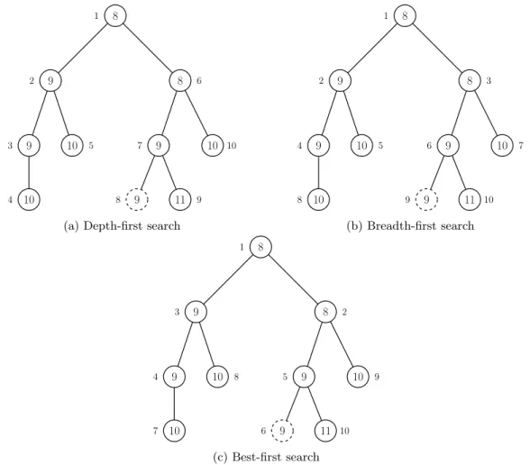
The search strategy in a B&B algorithm determines the order in which unexplored subproblems in T are selected for exploration. The choice of search strategy has potentially significant consequences for the amount of computation time required for the B&B procedure, as well as the amount of memory used. In some cases, for very large or challenging problems, it may be necessary to choose a search strategy that requires low memory usage; however, for problems in which memory is not a concern, other search strategies exist which may find an optimal solution very quickly, and thus explore potentially fewer subproblems. A comparison of some search strategies is given in Ibaraki (1976). In this section, a discussion of common search strategies, along with their strengths and weaknesses is given. Figure 2.3 shows a small search tree, and the order in which nodes are explored for several different search strategies.

8 9 9 10 8 9 9 11 10 10 1 2 3 4 5 6 7 8 9 10

(a) Depth-first search

8 9 9 10 8 9 9 11 10 10 1 2 3 4 5 6 7 8 9 10 (b) Breadth-first search 8 9 9 10 8 9 9 11 10 10 1 2 3 4 5 6 7 8 9 10 (c) Best-first search

Figure 2.3: Subproblem exploration order for different search strategies. The dashed subproblem is optimal, numbers inside nodes are subproblem lower bounds, and numbers outside the nodes indicate exploration order. The algorithm starts with an incumbent solution of value 10. BFS uses the lower bound as the measure-of-best, with ties broken arbitrarily.

(19)

2.2.1

Depth-First Search

Thedepth-first search(DFS) strategy (sometimes called depth-first search with backtracking, or last-in, first-out search; see Nemhauser and Wolsey, 1988, Section 11.4) is a search strategy used in many different graph algorithms in addition to B&B (Golomb and Baumert, 1965; Tarjan, 1972). It can be implemented by maintaining the list of unexplored subproblemsS as a stack. The algorithm removes the top item from the stack to choose the next subproblem to explore, and when children are generated as a result of branching, they are inserted on the top ofS. Thus, the next subproblem that is explored is the most recently generated subproblem.

However, a slight modification to this algorithm can be made to produce a substantial savings in memory usage. In particular, if the children of a subproblem can be ordered in some way, then DFS does not need to store the entire list of unexplored subproblems (which can grow quite large) over the course of the algorithm. Instead, the search strategy only stores the path from the root of T to the current subproblem; at each subproblem along this path, it also stores the index of the last-explored child subproblem. At the current subproblem, the next unexplored child is selected for exploration. If no unexplored children remain, the algorithmbacktracksto the closest ancestor node with unexplored children.

In addition to its low memory requirements, another advantage of DFS arises when solving integer programming problems (Section 2.6.1) that use the LP relaxations as lower bounds. Since most branching decisions in this setting do not change the structure of the LP relaxation significantly, the LP solver can often reuse information from the parent LP solution as a starting point for the child LP solution. This procedure is calledwarm starting, and is used in many commercial LP solvers (Atamt¨urk and Savelsbergh, 2005).

Two problems arise with the use of the DFS strategy. The first problem is that na¨ıve implementations of DFS do not use any information about problem structure or bounds, which means the search process can spend large amounts of exploration time in poor regions of the search space. A related phenomenon, called thrashing, occurs when different regions of the search space all fail for the same or similar reasons (Kumar, 1992). For instance, perhaps the presence of a single branching constraint always leads to infeasibility, but the algorithm must explore many more subproblems before the infeasibility is detected.

A different problem arises when the search tree is extremely unbalanced. In other words, if some optimal solutions are close to the root, but there exist long paths in T that do not lead to an optimal solution, DFS can (unluckily) choose many long, bad paths before it explores a path leading to an optimal solution. However, this computation time often could be avoided via pruning rules if the search strategy instead chose to explore a short optimal path first. In fact, this behavior of DFS was first noticed on problems where the search tree had unbounded depth (Slate and Atkin, 1983), but the same problem exists in trees with a few

(20)

extremely long paths.

A host of variants to the depth-first search strategy exist that attempt to overcome these limitations. One common variant is theiterative deepeningDFS algorithm (Korf, 1985), which imposes a limit on the depth of subproblems explored by DFS; if the search process is not able to prove optimality using this depth limit, the depth is increased and the search is restarted from the root. This ensures that the search does not spend unneeded time exploring extremely long paths in the search tree while retaining the low memory overhead of regular DFS.

Another algorithm calledinterleaved depth-first searchby Meseguer (1997) tries to overcome thrash-ing behavior by performthrash-ing depth-first search from multiple locations in the search tree at once. This strategy can be performed by sequentially selecting exactly one subproblem to explore from each different DFS path in the search tree before returning to the first search path. This algorithm can improve performance over standard DFS with a relatively limited increase in memory usage (a single stack needs to be maintained for each search path).

A third variant of DFS isdepth-first search with complete branching, which tries to exploit problem structure by selecting the next child subproblem to explore as the one with the best computed lower bound (Scholl and Klein, 1999). This method explores the search tree more intelligently, at the expense of increased memory usage, since all child subproblems must be generated when a subproblem is explored. However, if the tree has a relatively small branching factor, this increased memory usage is not likely to be significant.

2.2.2

Breadth-First Search

Breadth-first search(BrFS) is the opposite of DFS in that it is implemented with a first-in, first-out, or queue, data structure. BrFS explores all subproblems that are a fixed distance from the root before exploring any deeper subproblems. The BrFS strategy has the advantage of always finding an optimal solution that is closest to the root of the tree, thus operating well on unbalanced search trees. However, since complete solutions are usually at larger depths, BrFS is generally unable to exploit pruning rules that compare against the current incumbent solution. For this reason, the memory requirements for BrFS are often quite high, and it is generally not used in a B&B context. Two exceptions are in the presence of dominance relations (Section 2.4.2), which can prune effectively even in the absence of a good incumbent solution, and if a good incumbent solution can be found effectively by some other means, for example with a good heuristic search (Sewell and Jacobson, 2012). It is also worth noting that in the absence of pruning rules, the iterative deepening DFS strategy explores the same sequence of nodes as BrFS with substantially lower memory requirements.

(21)

2.2.3

Best-First Search

In settings where sufficient memory is available to store the entire unexplored search tree, the best-first search (BFS) strategy is often used. This strategy makes use of a heuristic measure-of-best function µ : 2X

→ R, which computes a value µ(S) for every unexplored subproblem, and selects as the next

subproblem to explore the one minimizing µ. If µ(S) _≤ minx∈Sf(x) for all S (that is, the

measure-of-best function never overestimates the best solution in a subproblem), the measure-measure-of-best function is admissible. In the presence of an admissibleµ, BFS is also called the A∗ _{algorithm (Dechter and Pearl,}

1985), or sometimesbest-boundsearch. BFS can easily be implemented by storing the list of subproblems in a heap data structure, using the value ofµas the key (Cormen et al., 2009).

There are many choices for the measure-of-best function; one common choice is a lower bound on the value of the best solution in the subproblem. If the lower bound is strongly correlated with the subproblem objective values, this measure-of-best will encourage exploration of subproblems with better solutions. How-ever, in practice, lower bounds may not be a good proxy for the objective function value. For example, in integer programming problems which use the LP relaxation as a lower bound, a small lower bound may just indicate that the structure of the problem allows the LP to “cheat” in ways that the IP cannot. To overcome this, other candidate measure-of-best functions are heuristics which estimate the quality of a solution, such as in Sewell and Jacobson (2012). Additionally, Shi and ´Olafsson (2000) use a probabilistic function called thepromising index to estimate the quality of a solution, and commercial solvers such as CPLEX use a heuristic function to estimate the objective value of a particular subproblem (IBM Corp., 2014).

Best-first search offers a number of significant advantages over DFS; because it is not tied to exploring one specific branch of the tree before any other, it is often able to find good solutions earlier in the search process. In fact, this notion has been formalized in a theorem by Dechter and Pearl (1985) that states that, assuming an admissible µwith no ties and no dominance relations, BFS explores the fewest number of subproblems of any search strategy that has access to the same heuristic function and other information. However, as observed in Sewell and Jacobson (2012), BFS does still have one potential drawback—if there exist many subproblems in T for which µ(S) =f(x∗_{), depending on the tie-breaking rule used, BFS may}

spend much time in middle regions of the search tree and never explore an optimal solution (see Figure 2.3c, in which nodes 3,4,and 5 are explored before the optimal solution is found). In this situation, BFS may be slower than some other strategy. To overcome this, many BFS implementations employ diving heuristics or other heuristic methods to drive a subproblem towards a new incumbent solution that can aid in pruning (Bixby et al., 2000; Achterberg et al., 2008).

(22)

2.3

Branching Strategies

The choice of branching strategy determines how children are generated from a subproblem. Branching strategies can be categorized into two groups: binarybranching strategies and non-binary, orwide, branch-ing strategies. Additionally, due to the prevalence of integer programmbranch-ing problems, there is a plethora of literature devoted to branching strategies in integer programming. These will be discussed separately at the end of the section.

2.3.1

Binary Branching

Binary branching strategies focus on subdividing a subproblemS into two mutually-exclusive, smaller sub-problems. For example, in the knapsack problem, which seeks a maximum-cost selection of items to fit inside a storage bin with fixed capacity, a binary branching strategy for a subproblem S selects some unassigned item and creates two branches, one in which the item is included in the knapsack, and one in which the item is excluded from the knapsack (Kolesar, 1967). Most binary branching strategies are variants of this idea. The standard integer branching scheme for integer programming in Section 2.6.1 is another binary branching scheme.

In some cases, the mechanism for performing the partitioning is more complicated. For the graph coloring problem (Section 2.6.2), Mehrotra and Trick (1996) use a branching rule that either adds edges or contracts vertices ofGin order to force a pair of non-adjacent vertices to either share same color or use different colors. Similarly, in the branch-and-price solver for the generalized assignment problem (Section 2.6.3, (Savelsbergh, 1997)), branching is performed by either including or excluding all schedules that assign a particular task to a worker.

2.3.2

Wide Branching

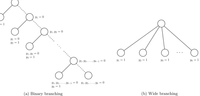
In contrast to binary branching are wide branching strategies, which focus on selecting one element from a set of different options. For example, in B&B algorithms to compute maximum cliques or independent sets in a graph, a set of unused vertices is maintained for each subproblem, and each unused vertex generates a child with that vertex added to the child’s set (Babel, 1994; Held et al., 2012). Wide branching methods allow for potentially large reductions in the size of the search tree. In the above example, a binary branching strategy would have to consider each unused vertex individually, creating a long sequence of subproblems. This long sequence can be bypassed with the wide branching technique (see Figure 2.4).

(23)

ordered sets(SOS), introduced by Beale and Tomlin (1970) and Beale and Forrest (1976). There are two types of special ordered sets, denoted by SOS1 and SOS2. An SOS1 is a set of elements for which at most one element can be used in a solution, and an SOS2 is a set of elements for which at most two adjacent elements can be used in a solution. SOS2 are useful for modeling piecewise linear approximations of nonlinear optimization problems (de Farias, Jr. et al., 2000; D’Ambrosio and Lodi, 2011). Wide branching strategies can be used in B&B to handle problems with SOS variables; for example, when an SOS1 is selected for branching, the strategy creates one branch for each element in the set. The subproblem for this set uses the chosen element and excludes all others. Finally, the branching strategy creates one subproblem which uses no elements from the set. This strategy can be generalized to handle SOS2, as well.

...

y1= 0 y1, y2= 0 y1, y2, . . . , yk−1= 0 y1= 1 y1= 0 y2= 1 y1, y2= 0 y3= 1 y1, y2, . . . , yk−1= 0 yk= 1 y1, y2, . . . , yk= 0

(a) Binary branching

y1= 1 y2= 1 y3= 1 yk= 1

. . .

(b) Wide branching

Figure 2.4: Binary branching versus wide branching. Given a set of k elements from which one must be selected, binary branching must explicitly reject elements 1,2, . . . , j −1 before creating a branch that considers elementj. Conversely, wide branching can consider each of them immediately.

Two potential problems arise with wide branching strategies. The first is that such strategies usually do not create mutually-exclusive branches, so it is possible to arrive at the same subproblem from several dif-ferent paths. It is generally easy to work around this problem using a lexicographic ordering rule (Geoffrion, 1969), memory-based dominance rules (Sewell et al., 2012; Sewell and Jacobson, 2012), or nogood recording (See Section 2.4 for more details on nogoods and dominance).

A second problem arises if the number of branches that can be created at a particular subproblem is very large. In this case, the algorithm could get stuck generating children at a particular subproblem and never move on to explore new regions of the search space. Moreover, if the number of generated children is very large at every subproblem, the size of the search tree will grow much more rapidly. There are two potential

(24)

ways around this issue; the first sets an arbitrary cap on the number of children that can be generated at a subproblem. If the branching factor ever exceeds this limit, any additional children are just discarded. This technique, used in the simple assembly line balancing solver of Sewell and Jacobson (2012), can prove optimality if the branching factor is never exceeded; otherwise, it performs as a heuristic. The other method uses adelayed branching technique, described in Section 5.1.2, in which the algorithm delays generation of the remaining children in the hopes that when it returns to the node, better bounds may have been computed that allow it to prune children more effectively.

Finally, a hybrid approach between binary branching and wide branching, called orbital branching, creates a large number of children when a subproblem is explored, but uses a group-theoretic concept of an orbitto prune off all but two of them. This technique is most useful for problems which demonstrate a high degree of symmetry (Ostrowski et al., 2011).

2.3.3

Branching in Integer Programs

Given that many optimization problems can be modeled using integer programming (Section 2.6.1), sub-stantial effort has been devoted to branching strategies for integer programming problems. The branching strategy is generally divided into two phases: selecting a variable or set of variables to branch on, and creat-ing child subproblems by imposcreat-ing bounds on these variables to force them away from fractional values. The choice of branching variable can significantly impact the performance of the algorithm, and many different techniques exist to choose good branching variables.

One commonly-used, easy-to-implement rule is called themost fractionalrule, which selects the variable yi whose fractional part is closest to 0.5 as the branching variable. However, as shown by Achterberg

et al. (2005), this branching rule is no better than selecting a branching variable at random in terms of computational time required and number of subproblems explored. Therefore, a number of more advanced techniques have been proposed in the literature to improve the performance of B&B integer programming solvers. The opposite branching rule, the least fractional rule selectsyi such that its fractional part is

furthest from 0.5; this rule is less commonly used and is often outperformed by other methods (see, for example, Ortega and Wolsey (2003)).

Another approach is to branch on variables that induce the most change in the objective function (Lin-deroth and Savelsbergh, 1999). There are two methods of doing this; the first, called strong branching, computes the LP relaxation objective value of the children of a subproblem S for each candidate branch-ing variable, and then selects the variable that induces the most change in the objective. However, this is computationally expensive, so an alternate method calledpseudocost branching (Benichou et al., 1971)

(25)

is often used which attempts to predict the per-unit change of the objective function for each candidate branching variable, based on past experience in the tree.

One problem that arises with pseudocost branching, however, is how to initialize the pseudocosts at the beginning of the algorithm, since no information is available about past behavior. To address this, a method called hybrid strong/pseudocost branching can be used, which employs strong branching at upper levels of the search tree to initialize the pseudocosts, and then uses pseudocosts in lower regions of the tree once more information is available. An alternate method, calledreliability branching proposed by Achterberg et al. (2005), uses strong branching for any variables whose pseudocosts have been deemed unreliable—that is, for which there is not enough historical information in the branching process to compute pseudocosts for the variable.

Recent research by Pryor and Chinneck (2011) has explored the use of branching rules that try to find fea-sible integer solutions to the problem quickly. They achieve this by branching on variables that induce change in the largest number ofvariablesin the problem (as opposed to the largest change in objective value, as with pseudocost branching). The somewhat surprising result in their paper shows that branching on variables with the smallest probability of satisfying constraints in the LP often leads to integer feasibility more quickly, because this will require a large number of other variables in the LP to change to satisfy the constraints.

Another recent branching method developed by Fischetti and Monaci (2011) is calledbackdoor branch-ing. This technique solves an auxiliary integer program to determine a small set of variables that should be branched on before any others; this auxiliary program is a set covering problem which computes a back-door—that is, a set of variables which, if branched upon early in the search process, yield a small search tree. Finally, Gilpin and Sandholm (2011) use information-theoretic results to guide the search process by branching so as to remove uncertainty from subproblems in the search tree. Subproblems close to the root in the search tree have a large amount of uncertainty, since few variables have been fixed; terminal subproblems have no uncertainty, since all variables have assumed integer values. To do this, they treat the values of fractional variables as probabilities, and compute the entropy (i.e., the amount of uncertainty) for each candidate branching variable, selecting the one with the least entropy to branch upon. A related technique by Karzan et al. (2009) uses machine learning techniques to train a B&B algorithm to choose branches that lead to small search trees.

(26)

2.4

Pruning and dominance rules

A critical aspect of B&B search is the choice of pruning rules used to exclude regions of the search space from exploration. Note that for a fixed branching strategy, any node that cannot be pruned by the pruning rules must be explored byanysearch strategy, even if an optimal solution is known before the search begins. The only way to reduce the size of the search tree in this case is to use better pruning rules. There are many different classes of pruning rules, but they are usually problem-specific and must be derived anew for each different problem type under consideration. Again because of its prevalence, many pruning rules are focused on integer programming problems.

2.4.1

Lower Bounds

The most common way to prune is to produce a lower bound on the objective function value at each subproblem, and use this to prune subproblems whose lower bound is no better than the incumbent’s solution value. Lower bounds are computed by relaxing various aspects of the problem. For example, in the simple assembly line balancing problem (Section 2.6.4) and its variants, one common relaxation is to compute the optimal solution value ignoring the precedence constraints (Vil`a and Pereira, 2014; Sewell and Jacobson, 2012). In general, as many different lower bounds can be computed as necessary; some lower bound computations may be easy to compute, whereas others may be more computationally intensive. Thus a common practice is to attempt to prune using the easy lower bounds first, and then move on to the more complex, but tighter, lower bounds if the easy methods are unsuccessful.

If the problem can be formulated as an integer program, the optimal value of the LP relaxation is an extremely common lower bound choice. The quality of the LP relaxation value is measured by the integrality gap of the formulation, that is, the ratio between the best integer solution and the best LP relaxation value across all problem instances. However, there may be many different ways to formulate the problem using integer programming, and some of these problems may have tighter integrality gaps than others. Thus, one technique for improving lower bounds is to derive a new formulation with a tighter integrality gap (Arora et al., 2002). The branch-and-cut and branch-and-price algorithms described in Sections 2.4.3 and 2.5 are common methods for exploiting integer programming formulations with tighter bounds. A related approach for polynomial programming problems called thereformulation-linearization technique(RLT) transforms a mathematical program with polynomial objective function and constraints into a linear program, and uses the resulting LP bound to prune in B&B algorithm to find global optimal solutions to the polynomial program (Sherali and Tuncbilek, 1992).

(27)

there is no strong duality theorem for integer programming, one can still arrive at a notion of weak duality. Given an integer program min{f(y) | Ay ≤b, y ∈ Z}, the Lagrangian relaxation problem is P(λ) =

min{f(y) +λ(b−Ay) | y ∈ Z}, where λ is a non-positive vector of real-valued weights calledLagrange

multipliers. The optimal solution value for the Lagrangian relaxation is always bounded above by the value of the optimal solution to the original problem. Thus, the best bound possible may be computed as the solution to the Lagrangian dual problem, maxλ≤0P(λ). The Lagrangian dual problem can be solved using subgradient optimization, a modification of Newton’s method for piecewise linear concave functions (Bertsimas and Tsitsiklis, 1997). Integer programming duality methods have been used in Vil`a and Pereira (2014); Desrosiers et al. (2013); Gendron et al. (2013), and Phan (2012), among others.

2.4.2

Dominance Relations

In contrast to lower bounding rules, dominance relations allow subproblems to be pruned if they can be shown to bedominatedby some other subproblem—in other words, if subproblemS1 dominates subproblemS2, this means that for any solution that is containedS2, there exists a complete solution inS1that is at least as good. Thus, it suffices to just exploreS1. Dominance relations, first studied by Kohler and Steiglitz (1974), are closely related to the Bellman equations from dynamic programming (Bellman, 1954). Note that, as shown by Ibaraki (1977), it is not always true that using dominance relations will improve the quality of the search process; however, there are many cases in which dominance relations will improve the search.

There are two primary types of dominance relations, memory-based and non-memory-based. Memory-based dominance rules compare unexplored subproblems to other problems previously generated and stored in the tree (Sewell et al., 2012). As the name implies, memory-based dominance rules require the entire search tree to be stored for the duration of the algorithm, instead of just the unexplored subproblems. However, this may allow for additional pruning to be performed that would be otherwise impossible.

Non-memory-based dominance relations do not require the dominating state to have been previously generated in the search process—instead, non-memory-based dominance rules are able to imply theexistence

of a dominating subproblem, regardless of whether it has been explored or generated. Such rules have the advantage that they do not require additional memory to store the generated search tree, but they may not be able to prune the same subset of problems that memory-based dominance rules can.

In B&B algorithms that employ dominance, the BrFS strategy has the useful property that it never explores a dominated subproblem, as long as the dominance relations are formulated in such a way so that subproblems are only compared if they are within the same level of T (see, for example, Nazareth et al. (1999); Sewell and Jacobson (2012)).

(28)

Note that care must be taken when implementing dominance rules to avoid mutual dominance relations. In particular, depending on the structure of the dominance rules employed, cycles of dominating subproblems S1, S2, . . . , Sk could exist where Si+1 dominates Si, and S1 dominates Sk (Demeulemeester et al., 2000).

In such cases, at least one subproblem in the dominance cycle must not be pruned; often, this can be accomplished using some lexicographic ordering rule.

2.4.3

Cutting Planes

The discussion in this section is restricted to problems that can be formulated as integer programs. A significant advance in the theory of linear and integer programming was developed by Gomory (1958), who introduced the idea of cutting planes. A cutting plane is a constraint that can be added to an integer program to tighten the feasible region without removing any integer solutions. This fundamental idea was applied to B&B by Padberg and Rinaldi (1991) to develop an algorithm called branch-and-cut. In this algorithm, new cutting planes (sometimes called valid inequalities) are added to the LP relaxation at every subproblem in the search tree (note that a valid inequality is a global constraint—it must apply at the LP relaxation of the root subproblem). The algorithm of Padberg and Rinaldi (1991) is specific to the well-known traveling salesman problem, but in Balas et al. (1996a) a generalization of branch-and-cut for binary integer programs is presented.

There are a number of different types of valid inequalities; an overview is given in Cornuéjols (2008). The initial cutting planes described by Gomory are calledGomory cuts, and are based on the structure of the simplex tableau. These cuts were shown to be of both practical and theoretical interest by Balas et al. (1996b). Some other types of valid inequalities are Chvátal-Gomory cuts(Letchford and Lodi, 2002), disjunctive cuts(Balas, 1979), andlift-and-projectcuts (Lovász and Schrijver, 1991; Balas et al., 1993). Of these, lift-and-project cuts provide an extremely general method to add valid inequalities, and thus are used in many different branch-and-cut algorithms (Balas and Perregaard, 2003). Lift-and-project operates by lifting the LP relaxation into a higher-dimensional space by adding additional variables, finding valid inequalities in this higher-dimensional space, and then projecting the valid inequalities back into the original space by deleting the extra variables.

Another method of generating valid inequalities is through decomposition methods such as Benders’ decomposition (Benders, 1962; Geoffrion, 1972). A decomposition method splits apart a problem into a master problem and one or more slave problems(sometimes referred to as “subproblems”, but this terminology is avoided herein to avoid confusion with the search tree subproblems). For example, in Benders’ decomposition, a set of complicating variables in the integer program are identified which drive the

(29)

intractability of the problem. The non-complicating variables are then projected out of the integer program. The master problem therefore seeks a solution to the new integer program, and the slave problem either determines that the master problem is feasible for the original integer program or produces a constraint that it violates. An algorithm to solve such a slave problem is also known as aseparation oracle, because

it separates feasible solutions from infeasible ones. These Benders’ cuts can then be added in to the

master problem. Hernández-Pérez and Salazar-González (2004) give an example of using Benders’ cuts in a branch-and-cut context to solve the traveling salesman problem with both pickups and deliveries.

One interesting question with regards to this method of pruning involves the interplay between cutting plane generation and branching. In many cases, the set of generated cuts is too large to allow all of them to be added, and it is often computationally expensive to generate new cuts, so at some point cutting planes are no longer generated and branching occurs. However, the question of when to stop generating cutting planes and start branching is an important problem when implementing a branch-and-cut algorithm (J¨unger et al., 1995; Mitchell, 2002).

2.4.4

Constraint Programming

Recently, interest has increased in using constraint programming techniques for solving optimization prob-lems. Constraint programming is a subfield of artificial intelligence that has been very successful in solving logic problems such as SAT. Constraint programming has many potential applications to B&B algorithms, and many other applications in optimization. For a complete discussion of the field of constraint program-ming and applications in AI and OR, see Rossi et al. (2006). Also, a comparison of constraint programprogram-ming and operations research techniques, along with an application of constraint programming to the fixed-charge network flow problem can be found in Kim and Hooker (2002).

Two primary ideas behind many constraint programming techniques for B&B algorithms areconstraint propagationand nogood learning(van Beek, 2006). Constraint propagation rules exploit the repeated application of logical inference rules in an attempt to derive contradictions that allow a subproblem to be pruned. On the other hand, a nogood is a structural property of the problem that has been proven to not lead to a feasible or optimal solution by complete exploration of some subtrees. Nogoods are generally learned over the course of the algorithm, and enable the search to check the validity of subproblems under consideration. Constraint programming techniques in B&B share many commonalities with other pruning techniques such as cutting planes and dominance relations. However, as pointed out by Caseau and Laburthe (1996), one significant difference is that constraint programming techniques are usually local techniques that tighten bounds at a particular subproblem, unlike the global pruning rules introduced by dominance or valid

(30)

inequalities.

An example of constraint propagation rules is given in Fahle (2002); in this paper, a technique called domain filteringis used to solve the maximum clique problem in a B&B context. Here, two results are proven showing when it is impossible for vertices in a graph to participate in a maximum clique, and these results are iteratively applied (orpropagated) at each subproblem inT. If the propagation reduces this list of candidate vertices to the empty set, the subproblem is fathomed.

Constraint propagation techniques often have close relations to lower bounding techniques. Fahle (2002) show that their domain filtering rule subsumes seven out of eight common lower bounds for the maximum clique problem. Moreover, Li et al. (2005) use a similar constraint propagation rule to aid in the computation of lower bounds that can be used for pruning in a Max-SAT solver (the Max-SAT problem seeks an assignment that satisfies the maximum number of clauses in a Boolean formula).

Conversely, nogoods are more closely related to dominance relations and cutting planes. For instance, Sandholm and Shields (2006) learn a sequence of nogoods (in this case, invalid assignments to sets of variables) that can be added as cuts to the integer program. These nogoods are derived by constraint propagation based on the branching decisions. Additionally, Fischetti and Salvagnin (2010) use nogood recording to develop dominance-like relations for a B&B solver for generic mixed-integer programming problems. Their solver uses an auxiliary integer programming problem to identify dominated subproblems; if a dominated subproblem is identified, it is stored as a nogood so that the auxiliary integer program for that subproblem does not need to be re-solved in the future.

2.5

Branch-and-Price

While B&B is useful in a wide variety of settings, a number of additional issues must be taken into con-sideration when the problem is very large. In this section, an extension of B&B called branch-and-price is discussed, which is applicable when the problem under consideration is formulated as an integer program with an exponential number of decision variables. However, since B&P is just an extension of B&B, the three core components (search strategy, branching strategy, and pruning rules) are still applicable in this setting. In a sense, B&P can be thought of as the dual algorithm to branch-and-cut (Section 2.4.3). Here, instead of adding new constraints to the (primal) master problem, a separation oracle for the dual of the master problem is used to add new constraints to the dual. This procedure is known as column generation, since new constraints in the dual of the master problem correspond to new variables (or constraint matrix columns) in the primal master problem. The column generation approach was first described in Dantzig

(31)

and Wolfe (1960), together with a decomposition method calledDantzig-Wolfe decomposition. Detailed descriptions of B&P algorithms are given in Barnhart et al. (1998) and L¨ubbecke and Desrosiers (2005), and pseudocode is presented in Algorithm 2.2.

The Dantzig-Wolfe decomposition method transforms an integer program into a new program where the variables correspond to the extreme points of the original IP. Since any solution to the original IP can be written as a convex combination of its extreme points, no information is lost. Moreover, in practice the reformulated program often yields much tighter bounds and less symmetry than the original. The principal drawback arises from the fact that the original IP has an exponential number of extreme points, which means that the number of variables (or columns) for the reformulated problem is too large to all be stored simultaneously. Therefore, to solve the LP relaxation and get a valid lower bound, column generation must be used.

In particular, if C is the (exponentially-sized) set of variables for the reformulated problem, a smaller problem called therestricted master problem(RMP) is solved over a subset C0 _{of the columns. Then,}

one or more slave problems (orpricing problems) are solved to identify new variables with the potential to improve the value of the LP relaxation, which can then be added to C0_{. The pricing problem is usually}

a weighted combinatorial optimization problem. The weights for the pricing problem are related to the optimal dual price vectorπ of the RMP, and the pricing problem identifies new variables (or columns) for inclusion inC0 _{by searching for}_C

∈C\C0_{with negative reduced cost. Note that in most cases, the pricing}

problem itself is NP-hard.

Algorithm 2.2:Branch-and-Price(X, f) 1 SetS ={X}

2 Initialize ˆxand the initial RMP poolC0 3 while S 6=_∅:

4 Select a subproblemS∈S to explore

5 if a solution ˆx0∈ {x∈S |f(x)< f(ˆx)}can be found: Set ˆx= ˆx0 6 if S cannot be pruned:

7 PartitionS intoS1, S2, . . . , Sr

8 for eachS_i∈ {S₁, S₂, . . . , S_r}:

9 hhColumn generation loop ii

10 while ∃C∈C \C0 with negative reduced cost atSi: AddCto C0

11 Compute a lower bound atSi using added columns

12 InsertS1, S2, . . . , Srinto S

13 RemoveS fromS 14 Return ˆx

Additional complexity arises when attempting to incorporate column generation with a B&B algorithm, because typical branching rules usually interfere with the structure of the pricing problem. In other words,

(32)

once some branching decisions have been fixed, new negative-reduced-cost variables must be found that respect the branching decisions. This problem, known as the constrained pricing problem, is closely related to thekth_{-shortest-path}_{problem. Moreover, when using standard integer branching rules (see Section 2.6.1)}

in B&P algorithms, there is often an asymmetry in the branching rule. For example, if the integer program contains a large number of covering constraints (of the form P_a

iyi ≥b), fixing a variable yi = 1 has the

potential to satisfy a large number of constraints, whereas fixing a variableyi= 0 may have minimal impacts

on the problem structure. This can lead to extremely unbalanced search trees, which in turn can impact the performance of the algorithm.

Therefore, to avoid interfering with the pricing problem structure and to attempt to create a more balanced search tree, most B&P algorithms use alternative branching strategies that do not disrupt the structure of the pricing problem. The branching strategy for graph coloring (Mehrotra and Trick, 1996) or for the generalized assignment problem (Savelsbergh, 1997) (see Section 2.3.2) are two such examples. Another general-purpose branching strategy for B&P algorithms involves branching on the original (non-decomposed) problem variables (Vanderbeck, 2011).

Due to the intractability of the pricing problem in many IP models, significant research has also gone into ways to solve the pricing problem. Gualandi and Malucelli (2012) use constraint programming techniques (Section 2.4.4) to more efficiently solve the pricing problem in a graph coloring B&P solver, and Easton et al. (2003) use a similar approach for a sports timetabling problem.

Finally, a new field of research is emerging in branch-and-cut-and-price algorithms, which use sep-aration oracles to produce new constraints for both the primal and dual master problems. These methods suffer from many of the same problems as B&P algorithms, since now the pricing problem must respect both the branching decisions and the additional cutting planes added to the problem. However, de Arag˜ao and Uchoa (2003) developed a new method calledrobust branch-and-cut-and-price(robust BCP) which further reformulates the master problem to eliminate the interference of cuts and branching decisions with the pricing problem. This method has been used with success in a number of vehicle routing and other graph problems (Fukasawa et al., 2006; Uchoa et al., 2008).

2.6

Problems of Interest

B&B methods are quite general, and thus the best way to gauge their performance in practice is to implement them for problems that are of practical or real-world interest. The techniques proposed in this dissertation are tested and validated against four different problems, which are described in the remainder of this section.

(33)

2.6.1

Mixed Integer Programming

The mixed integer programming problem is a very general NP-complete problem that can describe many different optimization problems using a set of algebraic constraints. Specifically, letybe a vector of variables, some of which are constrained to integer values. Also, letA be a real-valued matrix called theconstraint matrix, andb be a real-valued vector of constraint bounds. Then the search space for an integer program-ming instance is defined by the system of equationsAy≤b, with objective function f(y) =c0_{y, where}_c _is

a real-valued vector and0 _{denotes the transpose operator.}

In this setting, bounds are commonly produced by solving theLP relaxationof the problem, where the integrality constraints ony are relaxed. Branching decisions are imposed by adding additional constraints to the problem to shrink the feasible region without removing any optimal integral solutions. For example, the standard integer branching rule (sometimes called 0₋1 branchingify is a vector of binary variables) selects a variable yi with fractional value β in the LP relaxation and creates two new branches, one with

yi ≤ bβc (called a null assignment), and one with yi ≥ dβe (called a positive assignment). If no

fractional variablesyi exist, a new candidate incumbent has been found.

Many different optimization problems can be formulated as mixed integer programs, and the LP relax-ation often provides tight bounds in practice. Thus, a number of B&B techniques have been developed specif-ically for this setting. Moreover, many very efficient software packages (both commercial and freeware) exist for solving integer programs using B&B techniques, including CPLEX (IBM Corp., 2014), SYMPHONY (Ladanyi et al., 2014), Gurobi (Gurobi Optimization, Inc., 2014), LINDO (LINDO Systems, Inc., 2014), SCIP (Konrad-Zuse-Zentrum f¨ur Informationstechnik Berlin, 2014), and Xpress-MP (Fair Isaac Corporation (FICO), 2014).

There is a well-known database of mixe