Agricultural and Biosystems Engineering
Publications Agricultural and Biosystems Engineering
7-23-2019
Automated crop plant detection based on the
fusion of color and depth images for robotic weed
control
Jingyao Gai
Iowa State University, [email protected]
Lie Tang
Iowa State University, [email protected]
Brian L. Steward
Iowa State University, [email protected]
Follow this and additional works at:https://lib.dr.iastate.edu/abe_eng_pubs
Part of theAgriculture Commons, and theBioresource and Agricultural Engineering Commons The complete bibliographic information for this item can be found athttps://lib.dr.iastate.edu/ abe_eng_pubs/1065. For information on how to cite this item, please visithttp://lib.dr.iastate.edu/ howtocite.html.
This Article is brought to you for free and open access by the Agricultural and Biosystems Engineering at Iowa State University Digital Repository. It has been accepted for inclusion in Agricultural and Biosystems Engineering Publications by an authorized administrator of Iowa State University Digital Repository. For more information, please [email protected].
Automated crop plant detection based on the fusion of color and depth
images for robotic weed control
Abstract
Robotic weeding enables weed control near or within crop rows automatically, precisely and effectively. A computer‐vision system was developed for detecting crop plants at different growth stages for robotic weed control. Fusion of color images and depth images was investigated as a means of enhancing the detection accuracy of crop plants under conditions of high weed population. In‐field images of broccoli and lettuce were acquired 3–27 days after transplanting with a Kinect v2 sensor. The image processing pipeline included data preprocessing, vegetation pixel segmentation, plant extraction, feature extraction, feature‐based localization refinement, and crop plant classification. For the detection of broccoli and lettuce, the color‐depth fusion algorithm produced high true‐positive detection rates (91.7% and 90.8%, respectively) and low average false discovery rates (1.1% and 4.0%, respectively). Mean absolute localization errors of the crop plant stems were 26.8 and 7.4 mm for broccoli and lettuce, respectively. The fusion of color and depth was proved beneficial to the segmentation of crop plants from background, which improved the average segmentation success rates from 87.2% (depth‐based) and 76.4% (color‐based) to 96.6% for broccoli, and from 74.2% (depth‐based) and 81.2% (color‐based) to 92.4% for lettuce, respectively. The fusion‐based algorithm had reduced performance in detecting crop plants at early growth stages.
Keywords
computer vision, crop detection, robotic weeding, sensor fusion
Disciplines
Agriculture | Bioresource and Agricultural Engineering
Comments
This is the peer-reviewed version of the following article: Gai, Jingyao, Lie Tang, and Brian L. Steward. "Automated crop plant detection based on the fusion of color and depth images for robotic weed control."
Journal of Field Robotics(2019), which has been published in final form at DOI:10.1002/rob.21897. This article may be used for non-commercial purposes in accordance with Wiley Terms and Conditions for Self-Archiving.
1 Automated Crop Plant Detection Based on the Fusion of Color and Depth Images for Robotic
Weed Control
Jingyao Gai, Lie Tang, Brian L. Steward Abstract
Robotic weeding enables weed control near or within crop rows automatically, precisely and effectively. A computer-vision system was developed for detecting crop plants at different growth stages for robotic weed control. Fusion of color images and depth images was
investigated as a means of enhancing the detection accuracy of crop plants under conditions of high weed population. In-field images of broccoli and lettuce were acquired 3-27 days after transplanting with a Kinect v2 sensor. The image processing pipeline included data
preprocessing, vegetation pixel segmentation, plant extraction, feature extraction, feature-based localization refinement and crop plant classification. For the detection of broccoli and lettuce, the color-depth fusion algorithm produced high true positive detection rates (91.7% and 90.8%, respectively) and low average false discovery rates (1.1% and 4.0%, respectively). Mean absolute localization errors of the crop plant stems were 26.8 mm and 7.4 mm for broccoli and lettuce, respectively. The fusion of color and depth was proved beneficial to the segmentation of crop plants from background, which improved the average segmentation success rates from 87.2% based) and 76.4% (color-based) to 96.6% for broccoli, and from 74.2% (depth-based) and 81.2% (color-(depth-based) to 92.4% for lettuce, respectively. The fusion-based algorithm had reduced performance in detecting crop plants at early growth stages.
1 Introduction
Recently, with evolving consumer tastes, the interest in vegetables, especially natural, organic vegetables has grown (USDA, 2016, 2017). Compared with conventional farmers who control weeds using synthetic herbicides, organic farmers are mostly limited to non-chemical weed control strategies, of which, mechanical weeding methods such as hand weeding, tillage, and cultivation are common.
Mechanical weed control can be classified into two categories based on the target area of control relative to the crop row (Pannacci, Lattanzi, & Tei, 2017): 1) inter-row weeding (between crop rows), and 2) intra-row weeding (within or close to crop rows). Weeds between crop rows are relatively easy to control by mechanical cultivation. Intra-row weed control, however, is challenging because of the high risk of damaging crop plants when controlling weed plants close to the crop plants. Hand-weeding is commonly used, but it is laborious and costly. Although mechanical intra-row weeding machines are available, such as finger-weeders and torsion-weeders (Van Der Weide et al., 2008), they may damage crop plants unless they are accurately guided.
Robotic weeding becomes possible due to the evolution of perception systems,
especially computer vision technology. Research in computer vision for plant sensing has been documented over the past three decades and has led to the development of some robotic weeding machines. For instance, the Garford Robocrop InRow Weeder (Tillett, Hague, Grundy, &
Dedousis, 2008) detected crop plants with a color camera, and guided the disk hoes with a specially designed cutout to cut weeds around the detected crop plants. The Ladybird (Underwood et al., 2015) was a mobile robot that used various sensors such as LiDAR, hyperspectral imagers, and GPS for detecting and locating weeds. A 6-DOF robot arm with a spot sprayer was controlled accordingly. The Deepfield Bonirob (Lottes, Hörferlin, Sander, &
2 Stachniss, 2017; Ruckelshausen et al., 2009) detected crop plants with various of sensors (NIR, RGB cameras or Time-of-flight cameras), and treated weeds individually with a stamping tube. The AgBotII (Bawden et al., 2017) detected and classified weeds with a color camera, and control weeds with spot sprayers or hoeing tools.
Among the mechanical robotic weeding solutions, weeding efficacy can still be improved with better actuator design. As a part of this project, a new weeding actuator design for
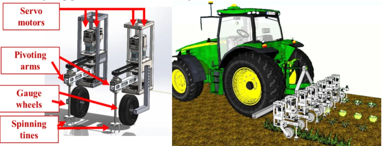
mechanical weeding for row crops and for multiple crop species was developed. The actuator was designed as an implement of a tractor. It employs rotating vertical tines as the weeding tool for effectively cutting, uprooting and burying weeds (Figure 1). The positioning of the times was controlled by servo-motor-driven pivoting arms. After detecting and localizing crop plants, the tines were controlled to move close to crop row to remove weed plants regardless of their species while avoiding crop plant disturbance and damage.
Figure 1. The actuators (left) were designed as an implement of a tractor (right), employing rotating vertical tines as the weeding tool for effectively cutting, uprooting and burying weeds.
In robotic weeding, precisely detecting, differentiating and localizing crop plants and weeds is still a challenging task. Feature-based supervised classification is a widely adopted technique in which computers usually use probability functions from digitized features in images to predict categories of objects. Since the shapes of plants are complex and varied, an effective and robust descriptor must differentiate different crop species from different weed plant species in images. More exploration is needed in this field.
Images for plant detection applications are commonly taken by two types of cameras. One type measures the intensity of light reflected from objects onto a discretized image plane. The other type of camera measures the distance between objects in the three-dimensional field-of-view and the sensor, and projects this range information onto an image plane.
Historically, most computer vision-based weed perception systems have used light reflectance images without depth information to identify plants (Slaughter, Giles, & Downey, 2008). Some work has focused on the different spectral reflectance features of plants and soil to distinguish between them. For example, the excess green index (ExG) and hue-saturation-value color space (HSV) were found effective in enhancing green plants in standard RGB images (Andújar, Weis, & Gerhards, 2012; Foglia & Reina, 2006; Philipp & Rath, 2002; Tang, Tian, & Steward, 2000). The normalized difference vegetation index (NDVI), which is a function of the near-infrared (NIR) and visible reflectance, was widely used in vegetation pixels segmentation when NIR sensors are available (Gerhards & Christensen, 2003).
3 engineered features representing the morphology of plant leaves and plant canopies for plant discrimination. These morphological features including length, width, perimeter dimensions, roundness, circularity, convexity and moment of plant leaves or plant canopy were widely used for feature-based plant identification (Mads Dyrmann, Christiansen, & Midtiby, 2018; Tang & Tian, 2008; Wu et al., 2007). Other than these features, general image features extractors such as Scale-invariant Feature Transform (SIFT), Features from Accelerated Segment Test (FAST), Histogram of Gradient (HOG), local binary pattern (LBP) and Gabor wavelet transformation, which are descriptors of local textures and key points, were also found effective in plant detection and discrimination, and robust to illumination variations (Bawden et al., 2017; dos Santos Ferreira, Matte Freitas, Gonçalves da Silva, Pistori, & Theophilo Folhes, 2017; Tang, Tian, & Steward, 2003).
In general, it is challenging for traditional methods with light reflectance sensors alone to obtain high discrimination accuracy under highly variable conditions, unless light was controlled and plants were sparse (Slaughter et al., 2008). Since most color cameras are passive receivers of reflected light, they are dependent on the quality of the reflected light received. The color
similarity of vegetation pixels can lead to difficulties in separating leaves or plants with occlusions, and uncontrolled illumination can cause shadow effects or saturation effects in images. Features extracted with such conditions may be incorrect and lead to incorrect plant identification results.
More recently, convolutional neural networks (CNNs) in deep learning have been applied in agricultural applications. The main advantage of CNN is the high performance in object detection and automated feature-engineering. CNN models such as Inception-v3 (Szegedy, Vanhoucke, Ioffe, Shlens, & Wojna, 2015), GoogleNet (Szegedy et al., 2014), DenseNet (Huang, Liu, Van Der Maaten, & Weinberger, 2017) and customized models were proven effective in crop/weed detection and classification even with uncontrolled illumination (M. Dyrmann, Jørgensen, & Midtiby, 2017; Mads Dyrmann, Karstoft, & Midtiby, 2016; McCool, Perez, & Upcroft, 2017; Milioto, Lottes, & Stachniss, 2017; Potena, Nardi, & Pretto, 2017).
CNN approaches, however, also face several challenges. First, deep learning requires high computational capacity for training and real-time inferencing. Second, deep learning has not been well integrated with prior knowledge so far, and it is difficult to engineer with, as indicated by Marcus (2018). The performance of deep learning depends on the quality of the datasets more than other conventional machine learning methods. The training dataset size must be sufficiently large to prevent overfitting, and that requires substantial manual labor to collect and annotate images. Also, the dataset must span all conditions such as inconsistent illumination, shadow and occlusion to improve robustness (Kamilaris & Prenafeta-Boldú, 2018). Thus, investigations of traditional pattern recognition pipelines are valuable and can provide a complementary approach particularly for applications with limited computational capacity and available datasets.
Range information, which reflects the 3D shape of objects, were found promising in addressing some of the problems in plant identification associated with color-based sensors alone. Specifically, 3D plant features such as edges and curvatures extracted from the 3D point cloud are more robust to external illumination condition changes than those extracted from color images. In addition, plant height can be an effective discriminating parameter between crop and weeds at early crop growth stages (Piron, van der Heijden, & Destain, 2011), which can be used for crop/weed segmentation and classification. Studies of crop or weed plant detection using range data have been reported. Three types of state-of-the-art range sensors were commonly used in agricultural applications, including stereo vision, light detection and ranging (LiDAR), and
4 time-of-flight (TOF) sensors (Weiss, Biber, Laible, Bohlmann, & Zell, 2010). Stereo vision extracts the distance between the sensor and objects in the field-of-view using images acquired with multiple cameras and exploits advantages of high image resolution, available color
information and detailed textural information (Kise, Zhang, & Rovira Más, 2005), while challenged by sensitivity to illumination and high computational requirements (Tippetts, Lee, Lillywhite, & Archibald, 2016). Jin & Tang (2009) demonstrated the use of a real-time stereo-vision system for corn seedling detection, in which the structural features of corn plants were extracted to identify the stem location of the corn plants at V2-V3 growth stages. Cameras with range sensors such as TOF sensors and LiDAR sensors measure distance based on the time difference between transmission and reception of typical infrared light signals. The active sensing mode makes these range cameras more robust to varying outdoor lighting conditions. In the work of Weiss et al. (2011), a robot (Deepfield Bonirob) was equipped with a LiDAR sensor to effectively map outdoor maize plants. Li et al. (2018) developed a TOF camera-based
perception system for crop plant detection. Features such as curvature, normal and neighbor counts were extracted from the 3D point cloud to detect broccoli and green bean leaves.
Since both color and range data can be beneficial, the fusion of color and depth images was explored for in-field crop/weed discrimination. Each image type has complementary information. Common sensors are color and depth sensors with calibrated extrinsic parameters (Herrera C., Kannala, & Heikkila, 2012), or commercial RGB-D camera such as Kinect (Microsoft, Redmond, Wash), which directly outputs registered RGB color and depth
information. The benefits of fusing color and range data were demonstrated in some agricultural applications. Nguyen et al. (2016) employed an RGB-D sensor to detect apples, in which 3D information was used for segmentation and clustering and color information was used to detect apples after circular Hough Transformation. In the study of Sa et al. (2017), an RGB-D sensor was used to detect sweet pepper peduncles for robotic harvesting. Kusumam et al. (2017) developed a mature broccoli head detection algorithm using an RGB-D sensor for robotic harvesting, and obtained a high detection rate. Xia et al. (2015) developed an algorithm to segment pepper leaves from complex background in greenhouses using a Kinect sensor. Andújar et al. (2016) employed a Kinect v2 sensor to estimate weed densities in corn fields. However, no studies reported on the fusion of color and depth to detect crop plants of multiple growth stages for the purpose of robotic weed control.
In this study, the benefits of fusing color and depth in crop plant segmentation for the automated weeding application was demonstrated. And a novel image processing pipeline for crop plant detection and localization by fusing color and depth images was developed and evaluated. The pipeline is adaptable to weeding robots which need to detect crop plants, such as in our design (Figure 1) and the Robocrop Weeder (Tillett et al., 2008). The image processing pipeline consists of several steps including data preprocessing, vegetation pixel segmentation, plant extraction, feature extraction, feature-based localization refinement and crop plant
classification. The algorithm is robust to high-density weeds. The primary objective of this paper was to evaluate the performance of the proposed pipeline in detecting and localizing crop plants at different growth stages. Specific research objectives were to:
• verify the fusion-based strategy will improve the segmentation performance compared with using color or depth only,
• evaluate the performance of the proposed fusion-based crop plant detection and localization algorithm at different critical processing steps, including segmentation, individual plant detection, and feature-based classification.
5
2 Sensor and data collection
2.1 Sensor
An RGB-D sensor (Kinect version 2, Microsoft, Redmond, Wash.)was used in this study, which provides color (RGB), infrared reflectance intensity and depth information. Depth was sensed using a semiconductor-based PMD TOF chip. The sensor contains three strong infrared light emitters, which enables the sensor to function under outdoor conditions when sunlight is not strong or has been reduced in intensity by shading. The sensing system outputs high
resolution RGB images at a 1920 × 1080 pixel spatial resolution, as well as infrared intensity and depth images at a 512 × 424 pixel resolution at 30 frames per second. At an outdoor working distance of 0.75-1.25 m with shaded sunlight, the standard deviation of the depth measurements was within 4 mm (Fankhauser et al., 2015). The systematic errors of Kinect v2 depth
measurements including depth distortion, amplitude-related error, temperature-related error and material-related error were estimated to be ±1 mm theoretically in this study (Corti, Giancola, Mainetti, & Sala, 2016; Fankhauser et al., 2015). Overall, the depth measurement uncertainty of the Kinect v2 sensor is within 5 mm (68% confidence level) by summing up the nonsystematic errors and systematic errors.
2.2 Data Collection
The target crop species analyzed were two common vegetable crops: lettuce (Lactuca, L.) and broccoli (Brassica oleracea L. var. botrytis L.). Various types of weeds that are common in Iowa were also in the scene, including bromegrass (Bromus inermis Leyss), pigweed
(Amaranthus spp.), lambsquarters (Chenopodium album), waterhemp (Amaranthus rudis), barnyardgrass (Echinochloa crus-galli), bindweed (Convolvulus arvensis), purslane (Portulaca oleracea), and white clover (Trifolium repens).
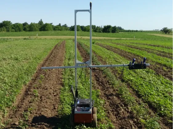
A data collection system, consisting of a Kinect v2 sensor and a laptop computer, was built on a remote-controlled ground vehicle (Figure 2). The sensor was placed about 0.75 m above the plants. With the selected working distance, the spatial resolution of depth was about 2 mm/pixel (12.5 ppi) in both vertical and horizontal directions while measuring the plants. The field of view was about 0.89 m (~34”) in vertical direction and 1.05 m (~41”) in horizontal direction (Figure 3).
6 Figure 2. Remote-controlled data collection apparatus in the horticulture research station of Iowa State University
Figure 3. The Kinect sensor was mounted at 0.75 m plus the estimated plant height above the field surface and had a 1.05 m by 0.89 m field of view of the plants and soil below.
Data were acquired at the Horticulture Research Station of Iowa State University in Story County (42.11 º N, -93.59 º E). The soil was close to Shunk River and nearly level. Soil type was
7 mostly Clarion loam, moderately eroded, with a five to nine percent slope. The average annual temperature was 49.45 ºF and the average annual precipitation was 0.91 m (35.83”). The crop plants used in this study (about 40 plants for each species) were started in a greenhouse and transplanted at the Horticulture Research Station. The row spacing was 0.76 m (30”), and the inter-row plant spacing was 0.3 m (12”). Weeding on the field was not fully performed in order to collect crop plant images from weed infested crop fields. The weed coverage was ranged from 5% - 50% of the imaged area.
Data were acquired with a Kinect v2 sensor in the summers of 2015 and 2016. For each crop plant species, images were taken at daytime about every five days from the date of
transplanting to maturity. More than 3,000 images were taken for each species. An umbrella was used to block the sunlight in sunny days to reduce the illuminance from above 80,000 lux to about 9,000 lux. In cloudy days, the average illuminance was about 35,000 lux, and no umbrella was used. Top view images were acquired every 0.3 m along the crop rows with the customized data collection system, and an overlap of 0.6 m between adjacent images was obtained. Depth images, near-infrared reflectance intensity images and color images were acquired.
3 Algorithm Design
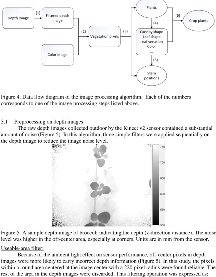
The acquired depth images from the depth sensor and RGB color images from the color camera were used as the inputs to the image processing algorithm. The framework of the detection and localization algorithm is shown in the flowchart (Figure 4) and can be outlined in the following steps:
Step 1: Preprocessing: This procedure removed invalid pixels and noise pixels in point clouds. A useable-area filter, a cut-off filter and a simplified neighbor count filter were used. Step 2: Segmentation: The background was removed by detecting the soil surface (assumed to be
a plane) using both color and depth information. Vegetation pixels were extracted. Step 3: Plant extraction: The vegetation pixels were separated into different clusters using their
spatial relationship. Each cluster represented one individual plant. These plants were localized as well.
Step 4: Feature extraction: Canopy and leaf features of each detected plant were extracted. Step 5: Feature-based localization refinement: The extracted features were used for refining the
localization and extraction results.
Step 6: Classification: Crop/weed classification was applied to all the separated plants based on their extracted features using machine learning techniques.
The algorithm was tuned and tested with broccoli and lettuce datasets collected at
different growth stages with weeds of different species and at different infestation levels. Each of these steps will be further described in the following sub-sections.
8 Figure 4. Data flow diagram of the image processing algorithm. Each of the numbers
corresponds to one of the image processing steps listed above.
3.1 Preprocessing on depth images
The raw depth images collected outdoor by the Kinect v2 sensor contained a substantial amount of noise (Figure 5). In this algorithm, three simple filters were applied sequentially on the depth image to reduce the image noise level.
Figure 5. A sample depth image of broccoli indicating the depth (z-direction distance). The noise level was higher in the off-center area, especially at corners. Units are in mm from the sensor. Useable-area filter:
Because of the ambient light effect on sensor performance, off-center pixels in depth images were more likely to carry incorrect depth information (Figure 5). In this study, the pixels within a round area centered at the image center with a 220 pixel radius were found reliable. The rest of the area in the depth images were discarded. This filtering operation was expressed as:
9 where src(x, y) is a pixel value in source depth image at position (column, row), and dst(x, y) is for a pixel in destination depth image. Position (256, 212) is the estimated principal point position of the camera. In this process, about 30% of the points were discarded.
Depth cut-off filter:
Invalid pixels (zero or infinity value) and pixels with large depth values (noise in most cases) were removed by using this filter. Through testing, a high threshold of the sensor height plus 200 mm was found robust to ensure the ground can be reserved. The low threshold was selected to be 500 mm, which is also the minimum working distance of the Kinect v2. The operation was expressed as:
𝑑𝑑𝑑𝑑𝑑𝑑(𝑥𝑥,𝑦𝑦) = �𝑑𝑑𝑠𝑠𝑠𝑠(𝑥𝑥,0 𝑦𝑦) 𝑖𝑖𝑖𝑖 500 <𝑑𝑑𝑠𝑠𝑠𝑠𝑜𝑜𝑑𝑑ℎ𝑒𝑒𝑠𝑠𝑒𝑒𝑖𝑖𝑑𝑑𝑒𝑒(𝑥𝑥,𝑦𝑦) <ℎ+ 200 (2) where (x, y) is the position of a pixel, and h is the sensor height in millimeter above the ground when taking this image.
Neighbor count filter:
The Kinect v2 depth sensor generates “flying pixels” at the edges of imaged objects (Figure 6), which are similar to blurred edges in 2D images. These pixels are sparse and have fewer “neighbors” in 3D space.
Since the output of the depth sensor of Kinect v2 was organized in rows and columns, simplified local radius-based neighbor search (RNS) was used to count neighbors in this study, which limited the searching process within a window in the images space of the depth image. The complexity was 𝑂𝑂(1), which is lower than the average complexity of 𝑂𝑂(𝑙𝑙𝑜𝑜𝑙𝑙𝑛𝑛) global k-d tree-based 3D searching algorithms. A window size of 5×5 was selected, and pixels that had horizontal distance (along the depth measurement direction) less than 15 mm were considered as adjacent pixels.
During filtering, neighbors for each pixel were calculated, then pixels with less than 15 neighbors were removed. This threshold was selected for a 5×5 searching window ensuring pixels on the edge were retained. The filtering operation were expressed as:
𝑑𝑑𝑑𝑑𝑑𝑑(𝑥𝑥,𝑦𝑦) = �𝑑𝑑𝑠𝑠𝑠𝑠(0 𝑥𝑥,𝑦𝑦) 𝑖𝑖𝑖𝑖𝑅𝑅𝑅𝑅𝑅𝑅𝑜𝑜𝑑𝑑ℎ𝑒𝑒𝑠𝑠𝑒𝑒𝑖𝑖𝑑𝑑𝑒𝑒(𝑥𝑥,𝑦𝑦) > 15 (3)
(a) Point cloud with sparse noise (b) Point cloud after filtering Figure 6. Corn plant sample images showing the differences before (a) and after (b)
preprocessing. The point clouds were generated from corn plants in the laboratory to illustrate the filtering process. After applying preprocessing procedure, the sparse noise was removed.
10
3.2 Segmentation using depth and color
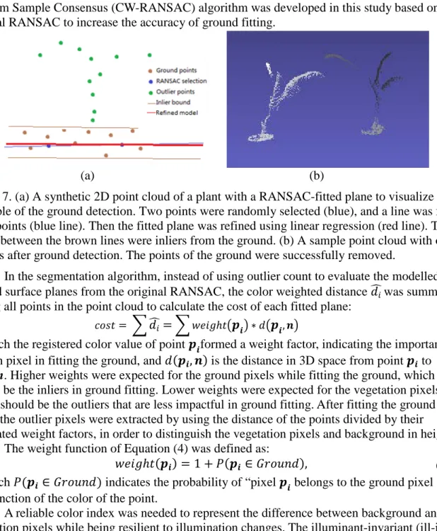
In segmentation, pixels were divided into two different subsets: vegetation pixels, and background pixels. With the depth information available, the main strategy of segmentation was to find the ground plane in the point cloud using Random Sample Consensus (RANSAC) (Weiss & Biber, 2011). RANSAC is widely used for model fitting with outliers (Figure 7 (a)). It
iteratively samples three random points in the point cloud to form a plane, and select the best plane with the least outliers. The model was refined with linear least squares regression. In fitting the ground plane, the soil surface should be inliers and the vegetation pixels should be outliers (Figure 7 (b)). However, when too many outlier points from plants are present, the original RANSAC will find an incorrect ground plane. To address this problem, a color-weighted
Random Sample Consensus (CW-RANSAC) algorithm was developed in this study based on the original RANSAC to increase the accuracy of ground fitting.
(a) (b)
Figure 7. (a) A synthetic 2D point cloud of a plant with a RANSAC-fitted plane to visualize the principle of the ground detection. Two points were randomly selected (blue), and a line was fit to these points (blue line). Then the fitted plane was refined using linear regression (red line). The points between the brown lines were inliers from the ground. (b) A sample point cloud with only outliers after ground detection. The points of the ground were successfully removed.
In the segmentation algorithm, instead of using outlier count to evaluate the modelled ground surface planes from the original RANSAC, the color weighted distance 𝑑𝑑�𝑖𝑖was summed among all points in the point cloud to calculate the cost of each fitted plane:
𝑠𝑠𝑜𝑜𝑑𝑑𝑑𝑑= �𝑑𝑑�𝑖𝑖=� 𝑒𝑒𝑒𝑒𝑖𝑖𝑙𝑙ℎ𝑑𝑑�𝒑𝒑𝒊𝒊� ∗ 𝑑𝑑�𝒑𝒑𝒊𝒊,𝒏𝒏� (4)
in which the registered color value of point 𝒑𝒑𝒊𝒊formed a weight factor, indicating the importance of each pixel in fitting the ground, and 𝑑𝑑(𝒑𝒑𝒊𝒊,𝒏𝒏) is the distance in 3D space from point 𝒑𝒑𝒊𝒊 to plane n. Higher weights were expected for the ground pixels while fitting the ground, which should be the inliers in ground fitting. Lower weights were expected for the vegetation pixels, which should be the outliers that are less impactful in ground fitting. After fitting the ground plane, the outlier pixels were extracted by using the distance of the points divided by their calculated weight factors, in order to distinguish the vegetation pixels and background in height.
The weight function of Equation (4) was defined as:
𝑒𝑒𝑒𝑒𝑖𝑖𝑙𝑙ℎ𝑑𝑑(𝒑𝒑𝒊𝒊) = 1 +𝑃𝑃(𝒑𝒑𝒊𝒊 ∈ 𝐺𝐺𝑠𝑠𝑜𝑜𝐺𝐺𝑛𝑛𝑑𝑑), (5) in which 𝑃𝑃(𝒑𝒑𝒊𝒊 ∈ 𝐺𝐺𝑠𝑠𝑜𝑜𝐺𝐺𝑛𝑛𝑑𝑑) indicates the probability of “pixel 𝒑𝒑𝒊𝒊 belongs to the ground pixel set,” as a function of the color of the point.
A reliable color index was needed to represent the difference between background and vegetation pixels while being resilient to illumination changes. The illuminant-invariant (ill-inv)
11 maps created based on the illuminant invariant color space (Finlayson, Hordley, & Drew, 2002) were found able to reduce the shadow effects within the original color image (Figure 8). The HSV (Hue-Saturation-Value) color space was also found reliable to distinguish green plants from the background (Hamuda, Mc Ginley, Glavin, & Jones, 2017). Thus, both ill-inv maps and the HSV color space image were selected to be candidates for calculating the weights.
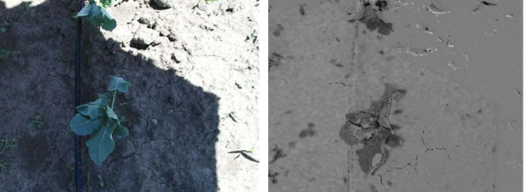
Figure 8: Sample illuminant-invariant map. In the left figure, the lighting conditions were different between the shaded and unshaded areas. In the right figure, the illuminant-invariant map was generated and removed the effects of changing lighting conditions. Green pixels had lower values in illuminant-invariant maps.
In this study, a logistic regression model with a sigmoid shape was used to determine the probability density function (PDF) in which is expressed as:
𝑃𝑃[𝑌𝑌= 1|𝑋𝑋=𝑥𝑥𝑖𝑖] = 𝑒𝑒 (𝛽𝛽0+𝜷𝜷𝟏𝟏𝒙𝒙𝒊𝒊) 1 +𝑒𝑒(𝛽𝛽0+𝜷𝜷𝟏𝟏𝒙𝒙𝒊𝒊) = 1 1 + exp(−𝛽𝛽0− 𝜷𝜷𝟏𝟏𝒙𝒙𝒊𝒊), (6) and could transform the color information into a 0 to 1 range. Scalar β0 and vector β1 are the
coefficients, and 𝒙𝒙𝒊𝒊 is a vector variable representing the color. The logistic regression was used for two reasons. First, the logistic response function curve is monotonically increasing or decreasing depending on the signs of 𝜷𝜷𝟏𝟏. The curve gradually approaches 0 and 1 after being approximately linear in the middle. Secondly, the logistic response function model is based on maximum likelihood estimation theory, and doesn’t rely on the assumptions of normally distributed error, equal variance of different parameters of data, and independently and identically distributed data which may not characterize the data. In addition, this model has a relatively low computational cost in fitting the model and calculating the probability.
For simplicity, the color vector variable 𝒙𝒙𝒊𝒊 in Equation 6 was selected from one of three color spaces: RGB, HSV and Illuminant-invariant. By analyzing the images acquired with our data collection system statistically (Gai, 2016), the most effective color space in distinguishing plants and soil surface were selected. The models of Equation 6 were fitted individually for broccoli and lettuce using the corresponding image set during the training phase, and used for segmentation during testing. With the dataset collected in this study, the RGB and the Illuminant-invariant color spaces were the most effective ones in plant segmentation for broccoli and lettuce, respectively. However, this may subject to change with the system working conditions such as soil types and shading methods.
3.3 Plant extraction
Segmented vegetation pixels were grouped into clusters representing individual plants based on the spatial relationship of pixels. In this step, an above-ground distance map was created, which replaced the values of the input depth image with the distance of each
12 corresponding point to the modeled ground plane. Clustering was applied on the created above-ground distance map, and the problem was reduced to a 2D unsupervised clustering problem on an image.
A 2D connected components method, which used a region growing schema, was used on the output mask of the segmentation step first for coarse clustering. After that, an algorithm based on the two-dimensional multi-scale wavelet transformation was applied on the above-ground distance map with a mask of the segmentation result, using prior knowledge of the shape patterns of crop plants. The Mexican hat wavelet was found effective in extracting shape patterns that are in spherical shape and isotropic. The normalized Mexican hat wavelet was defined as:
𝑧𝑧= (2−(𝑥𝑥2+𝑦𝑦2)/𝑑𝑑2)∗exp�−𝑥𝑥2+𝑦𝑦2
2𝑑𝑑2 �/𝑑𝑑2 (7)
in which parameter s is a scale factor, indicating the wavelet size. The Fast Fourier Transform (FFT) was used to reduce the computational cost of convolutions.
The wavelet transformation results at different scales were analyzed. The local extremes corresponded to the stem locations of individual crop plants, and the scales with maximum response at these local extremes corresponded to the plant canopy sizes. Vegetation pixels were associated with different clusters based on the plant stem locations and canopy sizes. These clusters indicated individual plants but without being labeled by their species tags yet.
Additionally, for plants without a spherical shape or not isotropic (e.g. the broccoli 13 days after transplanting (DAT) in this study), the plant extraction and localization will be refined using features extracted in the later steps.
3.4 Feature extraction
Plant discrimination was accomplished by feature-based classification. In this study, a series of hand-crafted features which represent the morphology and structure of plant canopies and leaves were extracted. In this section, the leaf and canopy features with their extraction methods are listed. Explicitly, the leaf extraction method and the leaf venation feature extraction method are stated in detail.
3.4.1 Plant features:
Inspired by the research of Wu et al. (2007), a set of morphological and structural features of plant leaves and canopies was selected in this study based on the consideration of feature distinguishability and algorithm simplicity. A program was developed to automatically extract the following features:
(1) Leaf venation, which is a Boolean variable, indicating whether the venation of the leaf can be extracted. The extraction method will be stated in the following section.
(2) Leaf height, which is the distance between the fitted ground and the centroid of the leaf. (3) Leaf area, which is the area of the leaf after projected to the ground plane.
(4) Leaf length, which is the maximum length on the leaf measured in 3D.
(5) Leaf width, which is the width of the leaf, perpendicular to the length direction, measured in 3D.
(6) Leaf aspect ratio, which is the ratio between thelength of the leaf, and width of the leaf. (7) Leaf roundness, which is the ratio between the leaf contour length and the bounding ellipse circumference, measured inside the image plane.
(8) Leaf rectangularity, which is the ratio between the leaf area and the leaf’s bounding rectangle area, measured inside the image plane.
13 the leaf pixels.
(10) Leaf saturation, which is the average saturation value in the HSV color space of the leaf pixels.
(11) Leaf illuminant-invariant value, which is the average ill-inv value of the leaf pixels. (12) Canopy height, which is the maximum distance from the ground plane to the highest point of the plant.
(13) Canopy radius, which is the size of the bounding circle of the canopy measured in 3D. (14) Leaf number, which is the number of leaves that can be segmented from the plant data. (15) Canopy hue, which is the average value of the hue channel in the HSV color space of the canopy pixels.
(16) Canopy saturation, which is the average value of the saturation channel in the HSV color space of the canopy pixels.
(17) Canopy illuminant-invariant value, which is the average illuminant-invariant value of the plant points.
3.4.2 Leaf segmentation:
Each leaf in the extracted plants was segmented to extract the leaf features (features 1 to 11). The marker-controlled watershed segmentation algorithm (Shafarenko, Petrou, & Kittler, 1997) was applied to both depth images and color images, specifically the HSV hue channel, to segment leaves. This general segmentation algorithm was used instead of using leaf shape as prior knowledge. Because leaf damage was common in the dataset collected, and the leaf shape patterns were not always available.
The “watersheds” in this study were the edges of leaves. The edges were defined by the discontinuities in depth and color. Those discontinuities were detected using the magnitudes of gradients in these images. In image processing, those partial derivatives were approximated by convolving Sobel operators to images for horizontal and vertical derivatives respectively. The magnitude of the gradient became the root of the square sums of the derivatives.
The label seed map was obtained from distance transformation to the edge map. The area with distance to the closet edges greater than a threshold was labeled with one of the foreground labels (label n, n>2). The pixels identified as background in previous steps were labeled as background (label 0). The rest of the pixels were labeled as unknown (label 1).
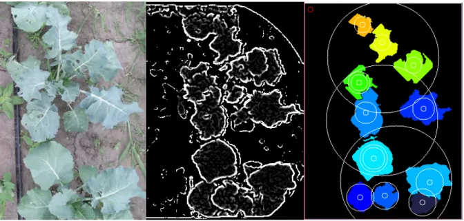
Then, the flooding algorithm was applied to the depth and color images, as well as the label seed map. An example resultant label image is shown in Figure 9. Based on the
segmentation results, features 2 – 11 can be extracted by analyzing the shape and color of each segment.
14 Figure 9. A run-time output example showing the leaf extraction procedures. Left: Color image from broccoli, with connected plants, slightly occlusions, as well as broken leaves. Middle: Combined gradient magnitude image on both color and depth. Right: Leaves extraction result example. Most of the leaves were extracted and labeled with different colors.
3.4.3 Venation extraction:
Venation (feature 1), as a leaf feature, was a distinguishing feature for crop plant
detection. It was resilient to most leaf damage and is a robust feature to determine the direction of leaves. As the pixels from veins usually have higher intensity in color images compared to surrounding pixels, those vein pixels were considered as “ridges” in the images. Ridge detection technique was applied to the color images. By limiting the processing areas to those leaves’ areas (obtained in leaf segmentation step), the veins were extracted, and a thinning algorithm (Chen & Hsu, 1988) was applied to skeletonize the veins (Figure 10).
Figure 10. An example run-time output of venation extraction methods. The left image is the raw image collected from the broccoli field. Leaf venation was found to be a robust feature to detect broccoli plants. The middle figure shows the map of reversed lower eigenvalues of Hessian
15 matrices of each pixel. Ridge pixels have higher intensity in the map. The right figure shows the extracted and skeletonized veins.
3.5 Feature-based localization refinement
In this step, the localization of plants in images was refined based on the features
extracted, especially the venations. A novel algorithm was developed in this study. Based on the observation that leaves of broccoli and lettuce plants are growing in pattern that radiates from the center of the canopy in top views, and thus the stems or the centers of the plants were localized by analyzing the leaves’ directions. Plant extraction results were refined by assigning extracted leaves to plants based on the leaves’ directions and their distances to the plant center.
Primary veins were found to be a reliable indicator of the leaves’ direction, and the stem location lies on the extension lines of the primary veins. Based on these observations, an
algorithm was developed to find the plant stem location using venations. The stem localization algorithm consisted of three steps:
1. Find all the vein branches, and fit line segments to them using least squares regression. 2. Estimate the probability of a line segment being a primary vein of a leaf, and assign a weight
factor to each line segment based on the probability.
3. Solve the center-finding problem by using the weighted robust least square method.
In the first step, all the branches were separated by finding joints and fitting line segments using least squares regression. In many binary skeletonizing algorithms with small thinning windows, the joints always follow some common patterns. For instance, in the algorithm of Chen & Hsu, (1988) all the joints were formed by patterns of either ‘Y’s or ‘T’s. After the joints were found, the vein branches/segments were separated.
The second step was to assign each line segment a weight factor, to reflect the probability of being a primary vein of a leaf. In most cases, a primary vein is the longest and has the most joints on it. In this step, for each line segment, the on-line joint count c was determined by counting joints who lie in the same leaf and have vertical distances less than five pixels to the line segment. Then the weight factor of each line segment was defined as the product of line segment length and a normalization function of on-line joint count c. The weight factor was defined as:
𝑒𝑒𝑒𝑒𝑖𝑖𝑙𝑙ℎ𝑑𝑑= 𝑙𝑙𝑖𝑖𝑛𝑛𝑒𝑒𝑑𝑑𝑒𝑒𝑙𝑙𝑠𝑠𝑒𝑒𝑛𝑛𝑑𝑑𝑙𝑙𝑒𝑒𝑛𝑛𝑙𝑙𝑑𝑑ℎ ∗ 𝑠𝑠𝑚𝑚𝑥𝑥𝑠𝑠𝑚𝑚𝑥𝑥 (1, 3 (1, 3∗ 𝑠𝑠∗ 𝑠𝑠)
𝑚𝑚𝑚𝑚𝑚𝑚) (8)
where cmax is the maximum on-line joint count found within the current leaf.
In the last step, an iterative weighted least square algorithm was used to find the stem location by finding a point who has minimum vertical distances to all the fitted line segments from primary veins. It iteratively activated and deactivated each line segment to ensure only inliers (ideally the primary veins) were used for fitting. For each iteration, the inlier line segments were activated, and the outlier line segments were deactivated. Then the center point was calculated by a weighted least square method, which solves:
𝒑𝒑=𝑚𝑚𝑠𝑠𝑙𝑙𝑠𝑠𝑖𝑖𝑛𝑛𝒑𝒑�(𝑒𝑒 ∗ 𝑑𝑑𝑖𝑖𝑑𝑑�𝒑𝒑,𝒍𝒍𝒋𝒋�)2 𝑗𝑗
(9) where p is the center point, ljis the j th activated line segment. With the new calculated center,
the distance of each line segment to the new center point was calculated. The mean and the standard deviation of the distances were calculated. Based on the mean and the standard
16 deactivated in the next iteration. The iterations continued until the center point reached the
desired accuracy. An example run-time output was shown in Figure 11.
Figure 11. A run-time output example of stem localization. Left: the venation skeletons of the lowest plant in Figure 10. Middle: the joints are colored in red, and the fitted line segments are drawn in green, with their lengths proportional to their weight factors. Right: the green cross indicates the resultant center location in the current iteration. The line segments with white color are the active (inliers, with non-zero weights in current iteration).
3.6 Feature-based Classification
Features extracted in the previous steps were used for crop/non-crop classification of each extracted plant. The classification was in a two-layer scheme, which is similar to the work of Dyrmann et al. (2018). The first layer consisted of a leaf/non-leaf classifier that used leaf features to exclude the incorrectly detected leaves from further classification. After classifying each leaf, for each separated plant, the classified crop leaf parameters were used to form a new set of predictors for the second classification layer. In this study, the statistical values including the maximum, minimum, mean, median, and standard deviation of each leaf feature in the same plant were formed as new predictor variables. The second layer was a crop/non-crop classifier that used the canopy features and the leaf features from classified leaves to classify each detected plant into the crop plant class or the non-crop plant class.
Among leaf features and canopy features, some features were found correlated. PCA (principal component analysis) was performed to reduce the dimension of these features before fitting models.
Eight supervised machine learning classification algorithms were applied to the features extracted in the training phase. These algorithms were: logistic regression (LR), k-nearest neighbors (KNN), artificial neural network (ANN), Bayes classifiers such as Linear and Quadrature Discriminant Analysis (LDA and QDA), the support vector machine (SVM), and tree-based classifiers such as random forest (RF) and Adaptive boosting (Adaboost). Then those models were evaluated by using Cross-Validation (CV) results. The image processing algorithm was implemented being written in C++ with calls to methods in the OpenCV library. The classification evaluation program was implemented using R language.
4 Experimental Design
The image analysis algorithm was applied, and the parameters were tuned with our broccoli and lettuce datasets collected in year 2015 and 2016. The performance of the developed algorithm was evaluated in terms of the accuracy of accomplishing three critical steps:
segmentation, plant detection and localization, and classification. The evaluation image set contained randomly selected 100 images for each species at five image collection time periods (3-7, 8-12, 13-17, 18-22, and 23-27 DAT), for a total of 500 images for each species. The crop
17 plant pixels and the crop plant stem locations in the evaluation image set were manually labeled for algorithm testing. The segmentation, plant detection and localization algorithms (Step 1 through Step 5 in Figure 4) were evaluated using the labeled evaluation image set. For classification (Step 6 in Figure 4), the models were trained using features from all the plants extracted after applying plant extraction algorithm (Step 1-5) to the entire image set, and evaluated using Cross-Validation.
4.1 Segmentation performance
Segmentation performance (after Step 2) was characterized by “segmentation success rate”, which is defined as the percentage of evaluation images segmented with IoU (Intersection over Union) greater than 75% (Long, Shelhamer, & Darrell, 2015). IoU greater than 75% indicates the ground plane was found correctly, and pixels from the crop plants were mostly extracted. The IoU was defined as:
𝐼𝐼𝑜𝑜𝐼𝐼= 𝑅𝑅𝑒𝑒𝑙𝑙𝑠𝑠𝑒𝑒𝑛𝑛𝑑𝑑𝑒𝑒𝑑𝑑𝑅𝑅𝑒𝑒𝑙𝑙𝑠𝑠𝑒𝑒𝑛𝑛𝑑𝑑𝑒𝑒𝑑𝑑𝑠𝑠𝑠𝑠𝑜𝑜𝑐𝑐𝑠𝑠𝑠𝑠𝑜𝑜𝑐𝑐𝑐𝑐𝑙𝑙𝑚𝑚𝑛𝑛𝑑𝑑𝑐𝑐𝑙𝑙𝑚𝑚𝑛𝑛𝑑𝑑𝑐𝑐𝑖𝑖𝑥𝑥𝑒𝑒𝑙𝑙𝑑𝑑 ∩ 𝐿𝐿𝑚𝑚𝐿𝐿𝑒𝑒𝑙𝑙𝑒𝑒𝑑𝑑𝑐𝑐𝑖𝑖𝑥𝑥𝑒𝑒𝑙𝑙𝑑𝑑 ∪ 𝐿𝐿𝑚𝑚𝐿𝐿𝑒𝑒𝑙𝑙𝑒𝑒𝑑𝑑𝑠𝑠𝑠𝑠𝑜𝑜𝑐𝑐𝑠𝑠𝑠𝑠𝑜𝑜𝑐𝑐𝑐𝑐𝑙𝑙𝑚𝑚𝑛𝑛𝑑𝑑𝑐𝑐𝑙𝑙𝑚𝑚𝑛𝑛𝑑𝑑𝑐𝑐𝑖𝑖𝑥𝑥𝑒𝑒𝑙𝑙𝑑𝑑𝑐𝑐𝑖𝑖𝑥𝑥𝑒𝑒𝑙𝑙𝑑𝑑 (10) After applying the segmentation algorithm to preprocessed images, successfully segmented (IoU > 75%) images of different growth stages were counted and compared.
4.2 Performance improvement verification
To verify the benefits of fusing depth and color in segmentation, two comparison experiments were conducted. To keep algorithm complexity consistent in the color-based method, the color PDF (Equation 6, with 0.5 as probability threshold) was applied to the color image to classify foreground and background pixels. One PDF function was fit using training dataset for each species, individually. The reason of not fitting multiple models for different growth stages was the motivation to test the robustness of the method against inconsistent illumination and other uncontrolled environment parameters. In the depth-based method, the original RANSAC algorithm was applied to the filtered depth image for segmentation. The algorithms were applied to the same dataset used by the proposed data fusion algorithm. Their performance was also evaluated using IoU-75%, and compared with the proposed fusion-based algorithm.
4.3 Plant detection and localization performance
The detection performance (after Step 5) was evaluated by the percentage of the crop plants extracted in the evaluation image set, which is the Recall, defined as True Positive / (True Positive + False Negative). Since all the crop plants were expected to be extracted, the Recall was expected to be 100%. The crop plants were characterized as correctly extracted if the IoU was greater than 50%, with which most of the features were found preserved. The localization performance was evaluated by the mean absolute error (MAE), which was calculated by
measuring the distance from the localization result to the labeled plant stem location in the image space, then calculated the real-world distances with the 3D point cloud. The error was named as “average crop plant localization error” in the following sections. In this study, the feature-based refinement was applied to broccoli 13 DAT, since the crop canopy shape was found
non-spherical and non-isotropic. The results of plant detection and localization, and the result after feature-based refinement at different growth stages were listed and compared.
4.4 Feature-based classification performance
The crop/non-crop classification performance (after Step 6) was evaluated using the minimized ten-fold CV (cross-validation) classification error. In this study, broccoli 13 DAT were found having extractable leaves with substantial features useful for crop/non-crop classification, so the two-layer classification method described before was applied. In the
18 classification of lettuce and broccoli less than 13 days, only canopy features were used, thus it is in a one-layer classification schema. Seven algorithms were applied to train models with the features extracted from the detected plants. During model tuning, about 10 preset values were selected for each parameter, and the models were examined with all parameter combinations to get the minimized CV errors. The overfitting problem was considered by monitoring both
training error and CV error during tuning. The best performance of each model was recorded and analyzed in terms of their ten-fold CV errors, and the training error.
5 Results and discussion
5.1 Segmentation performance and performance improvement verification
In the comparison experiments, with the depth-only segmentation algorithm, on average, 89.6% of the broccoli images and 74.2% of the lettuce images were segmented successfully (IoU > 75%, Equation 10). With the color-only segmentation algorithm, on average 77.4% of the broccoli images and 81.2% of the lettuce images were segmented successfully (IoU > 75%). With the color-depth fusion-based segmentation algorithm, on average 96.6% of the broccoli images and 92.4% of the lettuce images were segmented with IoU greater than 75%. The results for different DAT’s of different algorithms were listed in Table 1.
The fusion-based segmentation method showed higher segmentation performance in most tested situations than the color-based and depth-based algorithms with similar algorithm
complexity.
The failures of the depth-based algorithm mainly occurred in two scenarios. When too many outlier points or vegetation pixels were present, then the soil surface was barely visible, the RANSAC algorithm detected planes with points from plant leaves. Lower segmentation
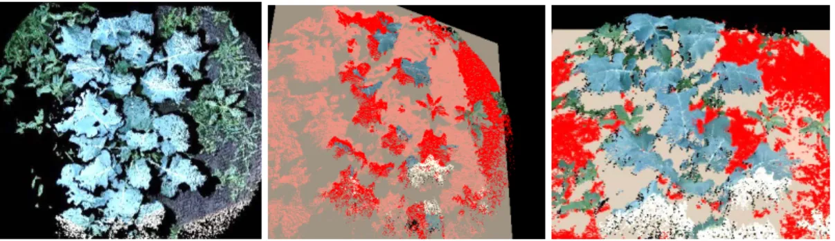
performance was also observed when the crops plants were low in height and the soil surface was not even, especially at early growth stages with the existence of ridges in the soil. In such situation, the target crop plants were likely to be segmented as background. Representative failure cases of the depth-based method were shown in Figure 12 and Figure 13.
Higher segmentation performance of the color-based method was observed in cloudy days, in which the ambient light intensity remained consistent in the image. In most failure cases, numerous vegetation pixels illuminated by the extreme high or low light intensity were classified as background, which usually happened in sunny days. Representative failure cases of the color-based method were shown in Figure 14.
The color-depth fusion method was more robust than the depth-based or the color-based method alone except when plants were at quite early growth stages. Specifically, the fusion-based method was more robust to high weed density than the depth-fusion-based method (Figure 13 (c)), and it is more robust to extreme lighting conditions than the color-based method (Figure 14 (c)). However, in this study, the fusion-based method still yielded a lower success rate than the color-based method at early growth stages (broccoli DAT<7, lettuce DAT<12). That was because some crop plants were even lower than the variation in the soil surface, and even with the color weight, they were segmented as background. Thus, at early growth stages (broccoli DAT<7, lettuce DAT<12), based segmentation was a better choice, and the results of the color-based method were used for the following steps.
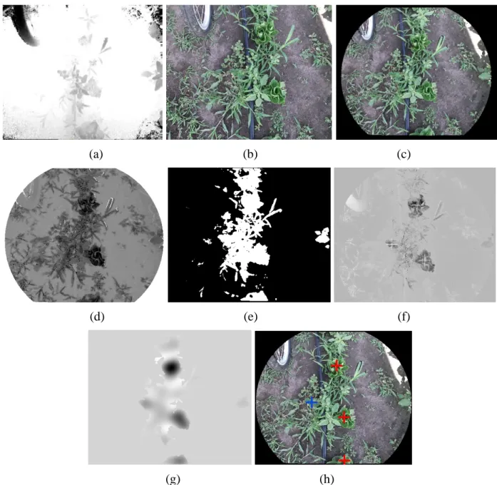
Additional examples of broccoli and lettuce segmentation results are shown in Figure 15-16 as step results of the entire image processing pipeline.
19 broccoli and lettuce at different growth stages. The human-measured average crop plant heights and weed densities at the corresponding data collection time were listed.
Days after transplanting 3-7 8-12 13-17 18-22 23-27 Average
Estimated weed coverage (%) 5-10 5-15 15-30 25-45 35-50 B ro cco li
Weather Cloudy Cloudy Cloudy Cloudy Sunny
Average Crop plant height (mm) 120 150 170 220 280 Fusion-based algorithm (%) 88 100 100 99 96 96.6 Depth-based algorithm (%) 68 100 100 81 87 87.2 Color-based algorithm (%) 100 100 81 84 26 76.4 L et tu ce
Weather Cloudy Cloudy Cloudy Sunny Sunny
Average Crop plant height (mm) 90 110 110 120 130 Fusion-based algorithm (%) 84 90 100 98 90 92.4 Depth-based algorithm (%) 54 63 80 91 83 74.2 Color-based algorithm(%) 100 100 95 52 59 81.2 (a) (b) Figure 12. A sample failure case of the depth-based algorithm (lettuce, 7 DAT). The algorithm failed to fit the correct ground plane and extract vegetation pixels in the point cloud (a), because the height contrast between soil and plants is not significant. Image (b) displays the segmentation result of the depth-based method. The fitted ground is displayed as a semi-transparent plane, and the segmented ground pixels were colored red. The results also cannot be improved by using the proposed fusion-based method.
20 (a) (b) (c)
Figure 13. A sample failure case of the depth-based algorithm (broccoli, 22 DAT). The algorithm failed to fit the correct ground plane and extract vegetation pixels in the point cloud (a) because of the high weed coverage. Image (b) displays the segmentation result of the depth-based method. Image (c) shows the corresponding improved result from the proposed fusion-based algorithm. The fitted ground is displayed as the yellow (transparent) plane, and the segmented ground pixels were colored red.
(a) (b) (c)
Figure 14. A failure case of the color-based algorithm (broccoli, 27 DAT) due to the extreme light conditions and shadow effects in image (a). Image (b) shows the color-based segmentation results, in which many saturated pixels were classified as background. Image (c) shows the corresponding improved result from the proposed fusion-based algorithm as a colored 3D point cloud, in which the color of segmented background pixels were colored red, and the color of vegetation pixels remain unchanged.
5.2 Plant extraction and localization
Without feature-based refinement, on average 87.6% of the broccoli plants and 95.2% of the lettuce plants were correctly extracted (Recall) at all growth stages. 69.1% and 87.4% of the detected plants were correct detections, which were actual broccoli or lettuce (Precision).
For broccoli images collected greater than 13 DAT, the plant extraction results were refined. The overall Recall of the broccoli plants extraction step was improved to 93.9%. The overall Precision of the broccoli extraction step was improved to 84.4%.
The average localization errors (MAE) of the crop plant stems after feature-based refinement were 26.8 mm and 7.4 mm for broccoli and lettuce, respectively. The average standard deviation of the localization errors were 6.8 mm and 2.4 mm for broccoli and lettuce, respectively.
It was observed that the error of plant extraction and localization increased as the crop plants grows (Table 2). Examples of broccoli and lettuce extraction and localization runtime results are shown in Figure 15 and Figure 16.
21 As an observation, before feature-based refinement, images with high weed densities or with large weed plants end up with larger localization error and larger mis-detection rate. This result was due to wrong plant detection by the blob detection algorithm and localization results with affection from weeds connected to the crop plants and some large weed plants. After feature-based refinement, which was applied to the broccoli 13 DAT, the accuracy of broccoli plant extraction and localization both improved. But since the venation extraction algorithm relied on the color information, it was still observed to be vulnerable to the inconsistent illumination problems, such as image saturation and shadow effects.
(a) (b) (c)
(d) (e) (f)
(g) (h) (i)
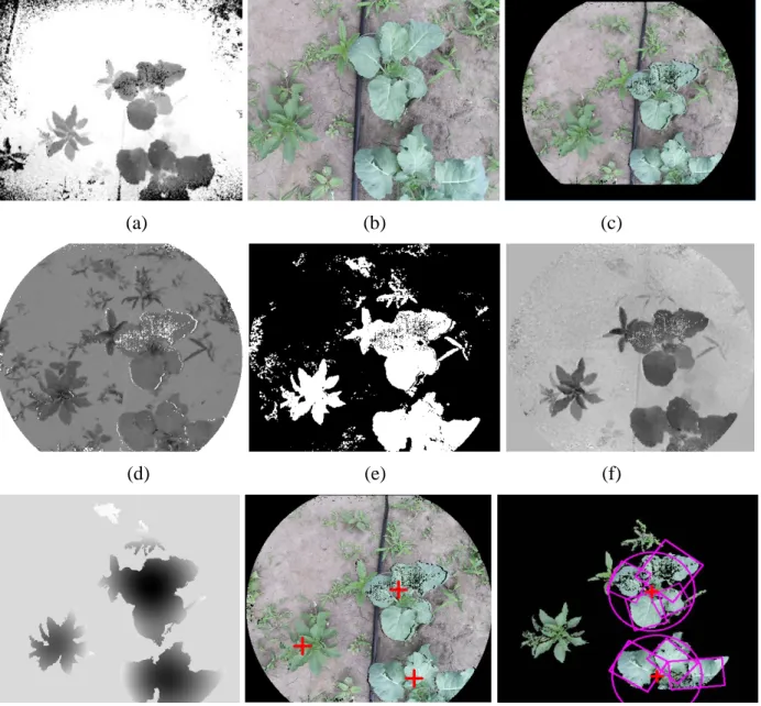
Figure 15. Sample broccoli plants images (16 DAT; 40k lux) at each image processing step including: (a) depth and (b) color images; (c) color registration and filtered image; (d) color-based weight map for segmentation; (e) segmented image, with white vegetation pixels; (f) above-ground distance map; (g) masked amplitude map of wavelet transformation; (h) detected
22 plants marked with crosses; and (i) feature-based localization refinement and classification with target crop plants labeled with crosses.
(a) (b) (c)
(d) (e) (f)
(g) (h)
Figure 16. Sample lettuce plants images (Taken at 22 DAT; 8k lux). (a) depth and (b) color images; (c) color registration and filtered image; (d) color-based weight map for segmentation; (e) segmented image, with white vegetation pixels; (f) above-ground distance map; (g) masked amplitude map of wavelet transformation; (h) crop plants detection and localization results marked with red crosses;
Table 2. The result of segmentation, plant extraction and localization steps for broccoli and lettuce at different growth stages.
Days after transplanting 3-7 8-12 13-17 18-22 23-27 Average
Estimated weed coverage (%)
23 B ro cco li Segmentation success rate (%) 100 100 100 99.0 96.0 99.0 Plant extraction Recall (%) 100 100 96.3 74.1 67.5 87.6 Feature-based refined extraction Recall (%) 100 100 98.2 87.1 84.5 93.9
Average crop plant localization error (MAE) ± standard deviation (mm) 10.2 ± 2.4 12.7 ± 2.2 14.1 ± 3.1 40.8 ± 9.7 52.6 ± 16.6 26.8 ± 6.8 L et tu ce Segmentation success rate (%) 100 100 100 98.0 90.0 97.6 Plant extraction Recall (%) 100 100 100 93.3 82.7 95.2
Average crop plant localization error (MAE) ± standard deviation (mm) 4.9 ± 1.5 5.2 ± 1.9 6.9 ± 2.0 9.4 ± 2.9 10.3 ± 3.5 7.4 ± 2.4 5.3 Classification
The feature extraction algorithm described in 3.4 was applied to the plant extraction results. In this study, for broccoli, 806 sets of canopy features 2858 sets of leaf features were extracted. For lettuce, 718 sets of canopy features were extracted. In the following subsections, the results were presented separately for broccoli classification and lettuce classification. Broccoli classification
As mentioned above, broccoli classification has two stages. One stage is leaf/non-leaf classification using leaf features, and the other is crop/non-crop classification. The minimized cross-validation (CV) errors of different methods in leaf/non-leaf classification are displayed in Table 3. In crop/non-crop classification, the canopy features as well as the classified crop-plant leaf features of each separated plant were used. As a result, the lowest average error rate
achieved in broccoli crop/non-crop classification was 3.1% during cross-validation, with the false positive rate of 1.1% and the false negative rate of 2.0% (Table 4).
Lettuce classification
Since only a few leaves can be extracted from the lettuce dataset, the crop/non-crop classification was performed by using only canopy features of the separated plants. As a result, the lowest average error rate achieved in lettuce crop was 6.8% in average in cross-validation, and with false positive rate of 4.0% and false negative rate of 2.8%. (Table 5).
Table 3. Model evaluation and comparison results of broccoli leaf classification. Listed are the minimized training errors, and CV errors, with the corresponding tuning parameters.
Model Tuning parameters Training error CV error
LR None 5.2% 8.6%
ANN Layer = (5, 2) 5.1% 15.4%
24 SVM Kernel = radial Gamma = 0.01 Cost = 100 5.3% 10.7% QDA None 6.4% 9.5% RandomForest N=500 13.8% 17.0% AdaBoost TreeDepth=4 Iter = 100 Nu = 0.2 5.7% 7.3%
Table 4. Model evaluation and comparison results of broccoli plant classification. Listed are the minimized training errors, and CV errors, with the corresponding tuning parameters.
Model Tuning parameters Training error CV error
LR None 7.2% 10.2% ANN Layer = (5, 2) 3.7% 11.9% KNN K=3 10.5% 14.3% SVM Kernel = radial Gamma = 0.01 Cost = 100 3.6% 5.6% QDA None 4.4% 10.4% RandomForest N=500 7.7% 8.4% AdaBoost TreeDepth=4 Iter = 50 Nu = 0.1 2.6% 3.1%
Table 5. Model evaluation and comparison results of lettuce plant classification. Listed are the minimized training errors, and CV errors, with the corresponding tuning parameters.
Model Tuning parameters Training error CV error
LR None 10.8% 13.4% ANN Layer = (5, 2) 8.3% 16.1% KNN K=5 9.9% 14.2% SVM Kernel = polynomial Gamma = 0.05 Cost = 10 7.2% 9.0% QDA None 7.9% 10.5% RandomForest N=500 8.4% 11.2% AdaBoost TreeDepth=4 Iter = 50 Nu = 0.1 5.1% 6.8%
Most of the classifiers were performing well in both stages of crop/non-crop
classification. Some non-linear parametric classifiers such as AdaBoost and SVM have slightly better performance. Thus, it can be concluded that the extracted features can represent the differences between crop and non-crop plants well. Several reasons that these non-linear classifiers performed better are: 1) The features extracted in this study created a non-linear decision boundary for examined plants. Crops are in the same patterns, and others are all non-crops. Linear models (LR, QDA) with sigmoid-shaped responses were not suitable because of
25 the models’ linear decision boundaries. 2) In this study, only about ten predictors were used after dimension reduction. Thus, Random Forest, which is mainly used with many predictors available and to find the most valuable features, was less suitable than non-linear SVM and AdaBoost. Further discussions about the failures about different classifiers will be studied in our further publications.
For the entire system, by combining the results of all the steps (plant extraction and feature-based classification), the system detected 91.7% of broccoli plants on average at all tested growth stages, and 1.1% of the detected broccoli plants were false positive. The average broccoli localization error was 26.8 mm. The system detected 90.8% of the lettuce plants, and 4.0% of the detected lettuce plants were false positive. The average lettuce localization error was 7.4 mm. The entire algorithm took about 300 ms for each image on a laptop with an Intel i7-4600m CPU. The implication is that the proposed algorithm on a regular PC will support travel at about 2 mph to detect and localize broccoli and lettuce with reported accuracy for a robotic weeding application.
6 Conclusions
In this paper, we proposed an image processing pipeline for detecting and localizing broccoli and lettuce crop plants by fusing color and depth images. For both crops (broccoli and lettuce) the detection algorithms produced high true positive detection rates (91.7% and 90.8%, respectively) and low average false discovery rates (1.1% and 4.0%, respectively). The average localization errors of the crop plant stems were 26.8 mm and 7.4 mm for broccoli and lettuce, respectively. The fusion of color and depth improved the average crop plant segmentation
success rates from 87.2% (depth-based) and 76.4% (color-based) to 96.6% for broccoli, and from 74.2% (depth-based) and 81.2% (color-based) to 92.4% for lettuce, respectively. The fusion-based algorithm had reduced performance in detecting crop plants at early growth stages. From the result of the experiments conducted, we can conclude that:
• The fusion of color and depth is beneficial to the segmentation of plants from background with same algorithm complexity at most tested growth stages. However, the fusion is less effective than using color only at early growth stages (broccoli DAT<7, lettuce DAT<12).
• Enhanced by the fusion of both color images and depth images, the crop plant detection algorithm was capable of detecting and localizing broccoli and lettuce plants at different growth stages with high weed densities in in the background of the images.
The framework of the proposed algorithm can be extended to different crop species, and the developed algorithm can be applicable to other applications such as selective spraying and plant mapping.
Acknowledgments
The research is sponsored by Leopold Center for Sustainable Agriculture, Grants No. M2009-23, M2012-24. USDA NIFA Foundational Programs, Grant No. 20136702121126
7 Reference
Andújar, D., Dorado, J., Fernández-Quintanilla, C., Ribeiro, A., Andújar, D., Dorado, J., … Ribeiro, A. (2016). An Approach to the Use of Depth Cameras for Weed Volume Estimation. Sensors, 16(7), 972. https://doi.org/10.3390/s16070972
Andújar, D., Weis, M., & Gerhards, R. (2012). An ultrasonic system for weed detection in cereal crops. Sensors (Switzerland), 12(12), 17343–17357. https://doi.org/10.3390/s121217343 Bawden, O., Kulk, J., Russell, R., McCool, C., English, A., Dayoub, F., … Perez, T. (2017).
26 Robot for weed species plant-specific management. Journal of Field Robotics, 34(6), 1179– 1199. https://doi.org/10.1002/rob.21727
Chen, Y. S., & Hsu, W. H. (1988). A modified fast parallel algorithm for thinning digital patterns. Pattern Recognition Letters, 7(2), 99–106. https://doi.org/10.1016/0167-8655(88)90124-9 Corti, A., Giancola, S., Mainetti, G., & Sala, R. (2016). A metrological characterization of the
Kinect V2 time-of-flight camera. Robotics and Autonomous Systems, 75, 584–594. https://doi.org/10.1016/j.robot.2015.09.024
dos Santos Ferreira, A., Matte Freitas, D., Gonçalves da Silva, G., Pistori, H., & Theophilo Folhes, M. (2017). Weed detection in soybean crops using ConvNets. Computers and Electronics in Agriculture, 143, 314–324. https://doi.org/10.1016/j.compag.2017.10.027 Dyrmann, M., Jørgensen, R. N., & Midtiby, H. S. (2017). RoboWeedSupport - Detection of weed
locations in leaf occluded cereal crops using a fully convolutional neural network. Advances in Animal Biosciences, 8(02), 842–847. https://doi.org/10.1017/S2040470017000206
Dyrmann, Mads, Christiansen, P., & Midtiby, H. S. (2018). Estimation of plant species by classifying plants and leaves in combination. Journal of Field Robotics, 35(2), 202–212. https://doi.org/10.1002/rob.21734
Dyrmann, Mads, Karstoft, H., & Midtiby, H. S. (2016). Plant species classification using deep convolutional neural network. Biosystems Engineering, 151, 72–80.
https://doi.org/10.1016/J.BIOSYSTEMSENG.2016.08.024
Fankhauser, P., Bloesch, M., Rodriguez, D., Kaestner, R., Hutter, M., & Siegwart, R. (2015). Kinect v2 for mobile robot navigation: Evaluation and modeling. Proceedings of the 17th International Conference on Advanced Robotics, ICAR 2015, 388–394.
https://doi.org/10.1109/ICAR.2015.7251485
Finlayson, G. D., Hordley, S. D., & Drew, M. S. (2002). Removing Shadows from Images. Computer Science, 2353(1), 823–836. https://doi.org/10.1109/TPAMI.2006.18
Foglia, M. M. M., & Reina, G. (2006). Agricultural robot for radicchio harvesting. Journal of Field Robotics, 23(6–7), 363–377. https://doi.org/10.1002/rob.20131
Gai, J. (2016). Plants detection, localization and discrimination using 3D machine vision for robotic intra-row weed control. Iowa State University.
Gerhards, R., & Christensen, S. (2003). Real-time weed detection, decision making and patch spraying in maize, sugarbeet, winter wheat and winter barley. Weed Research, 43(6), 385– 392. https://doi.org/10.1046/j.1365-3180.2003.00349.x
Hamuda, E., Mc Ginley, B., Glavin, M., & Jones, E. (2017). Automatic crop detection under field conditions using the HSV colour space and morphological operations. Computers and Electronics in Agriculture, 133, 97–107. https://doi.org/10.1016/j.compag.2016.11.021 Herrera C., D., Kannala, J., & Heikkila, J. (2012). Joint Depth and Color Camera Calibration
with Distortion Correction. IEEE Transactions on Pattern Analysis and Machine Intelligence, 34(10), 2058–2064. https://doi.org/10.1109/TPAMI.2012.125
Huang, G., Liu, Z., Van Der Maaten, L., & Weinberger, K. Q. (2017). Densely connected convolutional networks. Proceedings - 30th IEEE Conference on Computer Vision and Pattern Recognition, CVPR 2017, 2017-Janua, 2261–2269.
https://doi.org/10.1109/CVPR.2017.243
Jin, J., & Tang, L. (2009). Corn plant sensing using real-time stereo vision. Journal of Field Robotics, 26(6–7), 591–608. https://doi.org/10.1002/rob.20293
Kamilaris, A., & Prenafeta-Boldú, F. X. (2018). Deep learning in agriculture: A survey. Computers and Electronics in Agriculture, 147, 70–90.