Query Processing on Attributed Graphs

QUERY PROCESSING ON ATTRIBUTED GRAPHS

by

Ka Wai (Duncan) Yung

BEng in Computer Science, University of Hong Kong, 2009

MPhil in Computing, Hong Kong Polytechnic University, 2012

Submitted to the Graduate Faculty of

the Dietrich School of Arts and Sciences in partial fulfillment

of the requirements for the degree of

Doctor of Philosophy

University of Pittsburgh

2017

UNIVERSITY OF PITTSBURGH

DIETRICH SCHOOL OF ARTS AND SCIENCES

This dissertation was presented by

Ka Wai (Duncan) Yung

It was defended on Aug 11, 2017 and approved by

Dr. Shi-Kuo Chang, Department of Computer Science Dr. Alexandros Labrinidis, Department of Computer Science

Dr. Daniel Ahn, Department of Computer Science Dr. Konstantinos Pelechrinis, School of Information Science

QUERY PROCESSING ON ATTRIBUTED GRAPHS Ka Wai (Duncan) Yung, PhD

University of Pittsburgh, 2017

An attributed graph is a powerful tool for modeling a variety of information networks. It is not only able to represent relationships between objects easily, but it also allows every vertex and edge to have its attributes. Hence, a lot of data, such as the web, sensor networks, bi-ological networks, economic graphs, and social networks, are modeled as attributed graphs. Due to the popularity of attributed graphs, the study of attributed graphs has caught at-tentions of researchers. For example, there are studies of attributed graph OLAP, query engine, clustering, summary, constrained pattern matching query, and graph visualization, etc. However, to the best of our knowledge, the studies of topological and attribute relation-ships between vertices on attributed graphs have not drawn much attentions of researchers. Given the high expressive power and popularity of attributed graph, in this thesis, we define and study the processing of three new attributed graph queries, which would help users to understand the topological and attribute relationships between entities in attributed graphs. For example, a reachability query on a social network can tell whether two persons can be connected given certain attribute constraints; a reachability query on a biological network can tell whether a compound can be transformed to another compound under given chem-ical reaction conditions; a How-to-Reach query can tell why the answers of the above two reachability query are negative; a visualizable path summary query can offer an overall pic-ture of topological and attribute relationship between any two vertices in attributed graphs. Except for the proposed query types in this thesis, we believe that there is still penalty of meaningful attributed graph query types that have not been proposed and studied by the database and data mining community since an attributed graph is a very rich source of

infor-mation. Through this thesis, we hope to draw people’s attentions on attributed graph query processing so that more hidden information contained in attributed graphs can be queried and discovered.

ACKNOWLEDGEMENTS

I would like to thank my advisor, Prof. Shi-Kuo Chang, for the guidance during my study. He is always available to offer advice and support on any date and under any circumstance. I am very thankful that I can have Prof. Chang as my advisor.

It is my pleasure that I can have Prof. Alexandros Labrinidis, Prof. Daniel Ahn, and Prof. Konstantinos Pelechrinis serving on my Ph.D. committee. Thank you for giving me valuable advice on various research projects. All their advice are important to the completion of this work.

Love, understanding, and support from my family while I am away from home are in-valuable. Without their understanding and support, I believe that I would not be able to complete this study.

TABLE OF CONTENTS 1.0 INTRODUCTION . . . 1 1.1 Motivation . . . 1 1.2 Main Contributions . . . 2 1.3 Research Statement . . . 5 1.4 Thesis Organization . . . 5

2.0 BACKGROUND AND DEFINITIONS . . . 6

2.1 Definition of Attributed Graph and Attribute Constraint . . . 6

2.2 Primary-secondary Hybrid Storage Framework . . . 8

2.3 Query Processing System Framework . . . 8

3.0 LITERATURE REVIEW . . . 11

3.1 Attributed Graph Research . . . 11

3.1.1 Attributed Graph Query Engine . . . 11

3.1.2 Attributed Graph OLAP . . . 11

3.1.3 Attributed Graph Pattern Matching . . . 12

3.1.4 Attributed Graph Summarization . . . 12

3.1.5 Attributed Graph Clustering . . . 12

3.2 Graph Query Processing Research . . . 13

3.2.1 Reachability Query . . . 13

3.2.2 Reachability Query with Constraint . . . 14

3.2.3 Shortest Path Query . . . 15

3.2.3.1 Labeling-based Exact Methods . . . 15

3.2.3.3 Search-based Exact/Approximate Methods . . . 15

3.3 Why-Not Query Processing Research . . . 16

3.4 Graph Data Management System Research . . . 16

3.4.1 Semi-structured Data Managment System . . . 16

3.4.2 Graph Management System. . . 16

3.5 Advanced Graph Traversal Technique . . . 17

3.5.1 BFS/DFS . . . 17

3.5.2 A* Search and Landmark Technique . . . 17

3.6 Graph Visualization Technique . . . 17

4.0 FAST REACHABILITY COMPUTATION . . . 19

4.1 Motivation Application . . . 19

4.2 Challenges and Technical Contributions . . . 21

4.2.1 Chellenges . . . 21

4.2.2 Technical Contributions . . . 21

4.3 Problem Definition . . . 22

4.4 A New Approach for Constraint Verification . . . 25

4.4.1 Index Construction . . . 26

4.4.2 Query Algorithm . . . 28

4.4.2.1 Point Attribute Constraint Verification . . . 28

4.4.2.2 Set Attribute Constraint Verification. . . 28

4.4.3 Bounding Expected Number of Secondary Storage Access . . . 30

4.4.3.1 Point Attribute Constraint Query . . . 30

4.4.3.2 Set Attribute Constraint Query . . . 31

4.4.4 Discussion . . . 32

4.4.4.1 Hash Function . . . 32

4.4.4.2 Index Maintenance . . . 32

4.5 Heuristic Search Technique . . . 32

4.5.1 Index Construction for Heuristic Search . . . 33

4.5.2 Efficient Query Algorithm. . . 34

4.5.2.2 Guided Search . . . 34

4.5.2.3 Synopsis Update . . . 37

4.5.3 Proof of Correctness . . . 38

4.6 Optimization: Batch Attribute Retrieval Technique . . . 39

4.6.1 Index Construction . . . 39

4.6.2 Query Algorithm . . . 42

4.6.3 Bounding I/O . . . 43

4.7 Optimization: Better Utilization of Primary Storage . . . 44

4.7.1 Use of Extra Hash Values . . . 45

4.7.2 Attribute Selection Strategy . . . 46

4.7.2.1 Strategy1: Most Frequent . . . 46

4.7.2.2 Strategy 2: Maximum I/O . . . 47

4.7.2.3 Strategy 3: Lowest Entropy First. . . 49

4.8 Experimental Result . . . 49

4.8.1 Experiment Setup and Dataset . . . 49

4.8.1.1 Baselines . . . 49

4.8.1.2 Datasets . . . 50

4.8.2 Performance for Application Queries . . . 52

4.8.3 Performance on Real Graphs . . . 54

4.8.3.1 Experiment Design . . . 54

4.8.3.2 Result . . . 55

4.8.4 Performance on Synthetic Graphs . . . 56

4.8.5 Performance of Optimization Techniques . . . 56

4.8.5.1 Batch Attribute Retrieval . . . 56

4.8.5.2 Use of Extra Hash Values . . . 58

5.0 EFFECTIVE AND EFFICIENT HOW-TO-REACH ANSWER . . . . 68

5.1 Motivation Application . . . 68

5.2 Challenges and Technical Contributions . . . 69

5.2.1 Challenges . . . 69

5.3 Problem Definition . . . 71

5.3.1 Answer Quality . . . 71

5.4 Finding Optimal Answer . . . 73

5.4.1 Problem Of Applying Shortest Path Algorithm Directly . . . 73

5.4.1.1 Possible Decreasing Penalty. . . 74

5.4.1.2 Sub-optimal Answer Quality . . . 75

5.4.2 Attributed Graph Transformation . . . 76

5.4.2.1 Easy Implementation . . . 77

5.4.3 Proof of Optimal Answer Quality . . . 77

5.5 Station Index for Suboptimal Answer . . . 79

5.5.1 Station Index Construction . . . 79

5.5.1.1 Index Construction Algorithm . . . 79

5.5.1.2 Station Picking Strategy . . . 81

5.5.1.3 AttrSubPicking Strategy . . . 83

5.5.1.4 Space Consumption Analysis . . . 84

5.5.1.5 Time Complexity Analysis . . . 84

5.5.2 Efficient How-to-Reach Query Processing . . . 85

5.5.2.1 Hop Reduction . . . 85

5.5.2.2 Query Algorithm . . . 85

5.6 Experimental Result . . . 85

5.6.1 Experiment Setup and Dataset . . . 85

5.6.1.1 Experiment 1 - Comparison of Different Approaches . . . 88

5.6.1.2 Experiment 2 - Hop Distance to Nearest Station/Land-mark Analysis . . . 89

5.6.2 Performance on Real Graphs . . . 89

5.6.2.1 Query Time . . . 89

5.6.2.2 Penalty . . . 90

5.6.2.3 Hop Distance. . . 90

5.6.3 Performance on Synthetic Graphs . . . 90

6.0 VISUALIZABLE PATH SUMMARY COMPUTATION . . . 95

6.1 Motivation Application . . . 95

6.2 Challenges and Technical Contributions . . . 96

6.2.1 Challenges . . . 96

6.2.2 Technical Contributions . . . 97

6.3 Problem Definition . . . 97

6.3.1 Quality of Path Summary . . . 99

6.4 Path Summary Visualization Algorithm . . . 100

6.4.1 Algorithm Design . . . 100

6.4.2 Finding Key Vertices . . . 101

6.4.3 Finding Candidate Path. . . 101

6.4.3.1 Stitching Algorithm . . . 101

6.4.3.2 Candidate Path Search . . . 102

6.4.3.3 Conceptual Example . . . 102

6.4.4 Candidate Path Inflation . . . 104

6.5 Case Study and Evaluation . . . 107

6.5.1 Datasets . . . 108

6.5.2 Case Study . . . 108

6.5.3 Query Formulation Using Path Summary . . . 110

6.5.4 Change of Entropy . . . 112 7.0 CONCLUSION . . . 113 7.1 Summary of Contributions . . . 113 7.2 Intention . . . 114 7.3 Future Work . . . 114 7.3.1 Motivation . . . 114 7.3.2 Potential Direction . . . 115 8.0 BIBLIOGRAPHY . . . 117

LIST OF TABLES

3.1 Summary of Shortest Path Index Issue . . . 15

4.1 Summary of Frequently Used Symbols . . . 23

4.2 Worst Case Time and Space Complexity . . . 44

4.3 Attributes . . . 51

4.4 Dataset Information . . . 52

4.5 Parameter Setting . . . 52

4.6 Application Queries . . . 53

4.7 Results for Specific Queries (twitter−0.25) . . . 53

4.8 Results for Specific Queries (f b−bf s1). . . 54

4.9 Batch Retrieval Comparison . . . 57

4.10 Effect of Extra Hash Values . . . 59

5.1 Space Consumption. . . 84

5.2 Dataset Information . . . 86

5.3 Attributes . . . 87

5.4 Parameter Setting . . . 87

5.5 Expected Pros and Cons of Baselines . . . 88

6.1 Dataset and Parameter . . . 107

LIST OF FIGURES

2.1 Attributed Graph and Super-graph . . . 9

2.2 Primary-secondary Hybrid Storage Framework . . . 10

2.3 Potential Query Processing System Framework . . . 10

4.1 Attributed Graph and Super-graph . . . 24

4.2 Index Structure . . . 28

4.3 Choice of Path from s tot . . . 33

4.4 Example for Efficient Query Algorithm . . . 36

4.5 Batch Attribute Retrieval . . . 40

4.6 All Combinations of 3 Attributes . . . 47

4.7 [dblp]-Vary # of V Const. with Org. Dom. . . 56

4.8 [dblp]-Vary # of V Const. with Double Dom. . . 57

4.9 [dblp]-Vary # of E Const. with Org. Dom. . . 58

4.10 [dblp]-Vary # of E Const. with Double Dom. . . 59

4.11 [fb-bfs1]-Vary # of V Const. with Org. Dom. . . 60

4.12 [fb-bfs1]-Vary # of V Const. with Double Dom. . . 61

4.13 [fb-bfs1]-Vary # of E Const. with Org. Dom. . . 62

4.14 [fb-bfs1]-Vary # of E Const. with Double Dom. . . 63

4.15 [twitter-0.25]-Vary # of V Const. with Org. Dom. . . 64

4.16 [twitter-0.25]-Vary # of V Const. with Double Dom. . . 65

4.17 [twitter-0.25]-Vary # of E Const. with Org. Dom. . . 66

4.18 [twitter-0.25]-Vary # of E Const. with Double Dom. . . 67

5.1 Possible Decreasing Penalty . . . 75

5.2 Sub-optimal Answer Quality . . . 76

5.3 Optimal Answer Quality . . . 77

5.4 Station Index: s,t are served by nearby stations. . . 80

5.5 Vary Number of V Constraint . . . 91

5.6 Vary Graph Size . . . 92

5.7 [Real Graphs] Hop Dist to Nearest St/LM and Est. Space . . . 93

5.8 [SmallWorld]Hop Dist to Nearest St/LM and Est. Space . . . 94

5.9 [Erdos-Renyi] Hop Dist to Nearest St/LM and Est. Space . . . 94

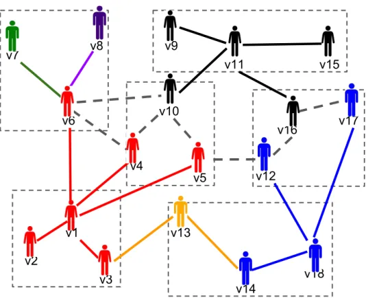
6.1 Path Summary (P1-blue, P2-orange) . . . 98

6.2 Stitching Algorithm (left) and Candidate Path (right). . . 104

6.3 a Candidate Path (left) and a Vertex Group Pi (right) . . . 107

6.4 Path Summary (Expected Num of Key Vertex=6, Num of Hint=3) . . . 110

6.5 Path Summary (Expected Num of Key Vertex=3, Num of Hint=1) . . . 111

LIST OF ALGORITHMS

1 Index Construction . . . 27

2 Check Constraint . . . 29

3 Efficient Query Algorithm . . . 35

4 Guided BFS . . . 37

5 Index Construction for Batch Attribute Retrieval . . . 41

6 Check Constraint using Batch Attribute Retrieval . . . 42

7 How-to-Reach Algorithm . . . 74

8 Station Index Construction . . . 81

9 Station Picking Strategy . . . 83

10 Stitching Algorithm . . . 103

11 Path Search Algorithm . . . 105

1.0 INTRODUCTION

1.1 MOTIVATION

Graph is a popular data structure that can efficiently represent relationships between objects. For example, in social networks, a user is represented by a vertex and social relationship such as friendship between two users is represented by an edge. However, unlike a tuple in a rela-tional table which has attributes, a vertex or an edge does not contain information about the object or relationship that they are representing. Fortunately, the emergence of attributed graph [1] remedies this drawback. In an attributed graph, every vertex and edge are associ-ated with a multi-dimensional attribute. The existence of attribute on every vertex and edge makes the graph capable of efficiently representing the relationship between objects as well as containing information of objects and relationships. That makes the expressive power of attributed graph to be very attractive for modeling a variety of information networks [2,1], such as the web, sensor networks, biological networks, economic graphs, and social networks. Due to the popularity of attributed graphs, the study of attributed graphs has caught attentions of researchers. For example, there are studies of attributed graph OLAP [1], attributed graph query engine [2], attributed graph clustering [3, 4], attributed graph sum-mary [5, 6, 7, 8, 9, 10, 11, 12, 13, 14] , constrained pattern matching query on attributed graph [15, 16], and graph visualization [17, 18]. However, to the best of our knowledge, the studies of topological and attribute relationships between vertices on attributed graphs have not drawn much attentions of researchers.

Answers of attributed graph path queries offer insight for understanding relationships between vertices since attributed graphs are rich in topological and attribute relationship information. For example, a social network can tell whether two persons can be connected

given certain attribute constraints; a biological network can tell whether a compound can be transformed to another compound under given chemical reaction conditions; an economic graph can tell whether an employee can be connected to an employee in rival company given certain constraint in employment history. Furthermore, by understanding the structure and attribute information between 2 entities on the attributed graph, it is also possible to tell why there is no such connection. Given that the relationships between entities on attributed graphs can be so meaningful, we believe that the studies of attributed graph path query would be an important piece in attributed graph research and building of attributed graph database systems.

1.2 MAIN CONTRIBUTIONS

In this thesis, we defined and proposed algorithms for answering three types of new at-tributed graph queries - atat-tributed graph reachability query, the How-to-Reach query, and the visualizable path summary query, which offer insights for users to understand topological and attribute relationships between vertices.

C1: Efficient Reachability Processing on Attributed Graph [19]The first contribu-tion of this thesis is an approach for effectively processing reachability query on attributed graphs.

• We introduced and defined the reachability query on attributed graph problem. Based on this definition, we developed our approach in a 2-level storage framework, which stores graph topology in primary storage (i.e. faster and smaller capacity, e.g. DRAM, PCM, local storage in distributed system) and attributes in the secondary storage (i.e. slower but larger capacity, e.g. magnetic disk, SSD, remote storage in distributed system). • We proposed a new constraint verification approach which takes the advantage of a

’perfect’ hash function [20, 21] for compressing a multi-dimensional attribute into a unique hash value. Such a compressed hash value always only requires a constant pri-mary storage space (no matter of attribute dimension and domain size) and is

suffi-gorithms (BF S, DF S, A∗ with Landmark [22]) is not required to access a distinct multi-dimensional attribute from the secondary storage more than once and ultimately, the primary storage space and expected number of secondary storage access can be theoret-ically bounded. Furthermore, the new approach allows constant CPU time and number of secondary storage access index maintenance, which would not impose a heavy burden on the overall performance of our approach for dynamic attributed graphs. This new constraint verification approach (hash index) can be used not only for our problem, but it can also be used by any graph traversal approach that involves attribute constraint verification.

• We proved theorems that can ensure the correctness of our new approach and we analyze the expected number of secondary storage access. We conclude that the expected number of secondary storage access for point attribute constraint query(Definition 15) is O(A) and for set attribute constraint query (Definition16) isO(Adif f×A), whereAis the size

of a multi-dimensional attribute and Adif f is the number of different multi-dimensional

attributes visited during graph traversal.

• We developed a heuristic search technique that takes into account graph structure as well as attribute distribution during graph traversal so as to reduce Adif f. The idea of

the heuristic search is to offer a direct passage that goes across graph regions that are likely to satisfy attribute constraints from source to destination. Also, the correctness of the heuristic search is theoretically proven. We emphasize that prevalent graph traversal techniques (e.g. BF S, DF S, A∗ with Landmark [22]) can all be used for our heuristic search techniques. Furthermore, the techniques that we proposed can be used for both directed and undirected graphs.

• We proposed two optimization techniques for further improving the efficiency of our new constraint verification approach. The first one is the batch attribute retrieval strategy which wisely retrieves verification material in batches. As a result, the batch attribute retrieval strategy can guarantee another worst case number of secondary storage access. The other one is a guidance for attribute selection strategy when extra primary storage is available for storing more hash values so that valuable primary storage space can be better utilized.

C2: How-to-Reach Query on Attributed Graph [23]The second contribution of this thesis is an approach for efficiently finding high quality sub-optimal for answering How-to-Reach query on attributed graphs.

• We introduced and defined a new How-to-Reach query which can be implemented in attributed graph database systems for improving databases’ usability. Since there may exist many attribute constraints that would allow source and destination to be connected, we further proposed a metric that would reflect the importance of attribute values for computing answer quality.

• We proposed a simple trick that 1)does not require heavy modification of existing im-plementations in graph database systems and 2)is proven to be able to allow existing shortest path algorithms to return optimal answers for How-to-Reach queries.

• Although after applying our trick, Dijkstra’s algorithm can return optimal answer for How-to-Reach queries, we observed that 1)the computation time of Dijkstra’s algorithm is unacceptable for inpatient users (i.e. ≈50sec) and 2)the hop distance of the optimals−t path tends to be meaningless (i.e. ≈1500 hops). Hence, to use such query in big graphs, we proposed the station index, which is a time and space efficient non-traversal based index that returns high-quality approximate answers with reasonable hop distances. C3: Visualizable Path Summary on Attributed Graph [24]The third contribution of this thesis is an approach for effectively computing visualizable path summary on attributed graphs.

• We introduced and defined the visualizable path summary query on attributed graph problem. We defined attributed path summary to be groups of vertices that contain users’ intuition as well as satisfy some path properties. The users’ intuition is expressed as hints for computing the path summary. Users can offer whatever attribute values that they consider as the hint. These summaries offer insight to users about the attribute values and connection between the given source and destination vertices.

• We proposed an efficient and effective approach for finding attributed path summary. Our proposed approach consist of three phrases. The first phrase efficiently finds all key

on those key vertices, a novel stitching algorithm is proposed to connect the source, the destination, and key vertices together to form a relatively small key vertex graph. After that, high-quality candidate paths between the source and the destination are found on that small key vertex graph efficiently. Finally, candidate paths are inflated to vertex groups by greedily including adjacent vertices.

1.3 RESEARCH STATEMENT

By defining basic attributed graph queries and developing techniques for efficiently and effec-tively answering basic attributed graph queries, meaningful applications that are related to topological and attribute relationship between vertices on attributed graph can be developed and answered effectively and efficiently.

1.4 THESIS ORGANIZATION

The rest of this thesis is organized as follow: Chapter2introduces background and definitions for this thesis. Chapter3 offers a literature review of all prior works that are related to this thesis. Chapter4presents all the details of our approach for efficiently answering attributed graph reachability queries. Chapter 5 presents all the details of our approach for efficiently and effectively answering attributed graph How-to-Reach queries. Chapter6presents all the details of our approach for effectively computing visualizable path summary for attributed graphs. Finally, Chapter 7 concludes this thesis.

2.0 BACKGROUND AND DEFINITIONS

In this chapter, we first define necessary notations and definitions used throughout the remainder of this thesis. After that, we introduce the primary-secondary hybrid storage framework utilized in this thesis.

2.1 DEFINITION OF ATTRIBUTED GRAPH AND ATTRIBUTE CONSTRAINT

Definition 1. [Attributed Graph] An attributed graph [1] G, is an undirected graph de-noted as G = (V, E, Av, Ae), where V is a set of vertices, E ⊆ V ×V is a set of edges,

and Av = (Av1, Av2, ..., Avdv) is a set of dv vertex-specific attributes, i.e. ∀v ∈ V, there

is a multidimensional tuple Av(v) denoted as Av(v) = (Av1(v), Av2(v), ..., Avdv(v)), and Ae = (Ae1, Ae2, ..., Aede) is a set of de edge-specific attributes, i.e. ∀e ∈E, there is a

multi-dimensional tuple Ae(e) denoted as Ae(e) = (Ae1(e), Ae2(e), ..., Aede(e)).

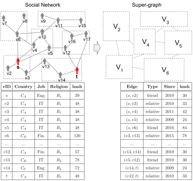
Figure2.1 is an example of attributed graph. It has a topology (V, E) and two attribute tables to store vertex attributes (Av, dv = 3) and edge attributes (Ae, de = 2). A super-graph,

which will be introduced in Chapter 4.5.1, is also shown in Figure 2.1.

Definition 2. [Vertex Attribute Value] Avi(v) is the value of the ith attribute of vertex v and is in the domain Dvi of attribute Avi.

Definition 3. [Edge Attribute Value] Aei(e) is the value of the ith attribute of edge e

and is in the domain Dei of attribute Aei.

Aei(e)∈Dei where Dei is the domain of Aei

For example, Av country(v2)=CA,Ae type((s, v2))=f riend.

Definition 4. [Vertex Attribute Value Set] Svi is a set of attribute value of Avi. Svi ⊆Dvi

Definition 5. [Edge Attribute Value Set] Sei is a set of attribute value of Aei. Sei ⊆Dei

For example, in Figure 2.1, Dv country = {CA, CB, CC, CD} and Sv country can be any

possible subset of Dv country e.g. Sv country ={CA, CB}.

Definition 6. [Vertex Attribute Constraint]Cv is a set of vertex attribute value setSvi. Cv ={Sv1, Sv2, ..., Svdv}

Definition 7. [Edge Attribute Constraint] Ce is a set of edge attribute value set Sei. Ce={Se1, Se2, ..., Sede}

For example, a vertex attribute constraint can be Cv ={{CA},{Eng., IT, F in.},{R1}}.

Definition 8. [Vertex Attribute Constraint Satisfy] Vertices in path p Av(p) satisfies

vertex attribute constraint Cv if and only if for all vertex v in p exclude s and t, every

attribute Avi(v) of v belongs to Svi, where Svi∈Cv.

Av(p)sat. Cv if f ∀v∈p\ {s, t},∀i= 1...dv, Avi(v)∈Svi,

where Svi∈Cv

Definition 9. [Edge Attribute Constraint Satisfy] Edges in pathp Ae(p)satisfies edge

attribute constraint Ce if and only if for all edge e in path p, every attribute Aei(e) of e

belongs to Sei, where Sei ∈Ce.

Ae(p)sat. Ce if f ∀e∈p,∀i= 1...de, Aei(e)∈Sei,

where Sei∈Ce

For example, in Figure 2.1, vertex s, v2, v3, v4, v5, v12, t satisfy the vertex attribute con-straint Cv ={{CA},{Eng., IT, F in.},{R1}}.

2.2 PRIMARY-SECONDARY HYBRID STORAGE FRAMEWORK

A pure in-memory solution does not scale well for graph query with attribute constraints. That is because attributed graphs consist of topology as well as attributes for every vertex and edge. For a large graph with 1 billion vertices, 3 billion edges, and 10 attributes for each vertex and edge, the size of all attributes is around 223 gigabytes (4 bytes per integer), which usually does not fit in primary storage (e.g. memory). Hence, it is unrealistic to assume that both topology and attributes of a big attributed graph can be always fit in primary storage. In this thesis, a primary-secondary hybrid framework [2] is adopted for efficient attributed graph query processing. Figure 2.2 is the framework. In this framework, the entire graph topology is stored in the primary storage (e.g. memory or local storage) while vertex and edge attributes are stored in the secondary storage (e.g. disk or remote storage). This framework can also be viewed as a two-level storage hierarchy. The first level has faster read/write speed but smaller storage capacity; the second level has slower read/write speed but larger storage capacity.

2.3 QUERY PROCESSING SYSTEM FRAMEWORK

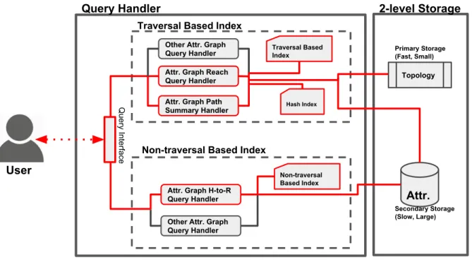
Figure 2.3 shows a potential query processing system framework that includes our contri-butions (red components) in this thesis. The system contains traversal based index and non-traversal based index for answering attributed graph queries. Both indexing approach consist of the query handler component and the index component. The query handler com-ponent controls how the query is answered and how the index is used; the index comcom-ponent offers services and information for the query handler component to compute the query an-swer. For traversal based indexing approach, there is the hash index component. This component offers indexing information for reducing number of secondary sotrage access of attributed graph traversal.

v2 v3 v5 v4 v10 v13 v12 v6 v14 v7 v8 v9 _v11 v16 v17 v15

s

t

V

V

V

V

V

V

Social Network

Super-graph

vID Country Job Religion hash

s CA Eng. R1 39 v2 CA IT R1 48 v3 CA IT R1 48 v4 CA IT R1 48 v5 CA IT R1 48 v6 CD Fin. R3 120 ... ... ... ... ... v10 CB Fin R1 60 v12 CA Fin. R1 57 v13 CB IT R2 78 v14 CC Eng. R2 72 t CA IT R1 48

Edge Type Since hash (s, v2) friend 2010 30 (s, v3) relative 2010 33 (s, v4) relative 2011 42 (s, v5) relative 2009 24 (s, v6) friend 2016 84 (v3, v13) relative 2015 78 (v4, v6) relative 2015 78 (v5, v10) relative 2015 78 (v4, v10) relative 2015 78 ... ... ... ... (v12, v16) friend 2016 84 (v13, v14) friend 2010 30 (v5, v12) friend 2010 30 (v14, t) relative 2009 24 (v12, t) relative 2010 33 (v17, t) friend 2016 84

Secondary Storage

Primary

Storage

Algorithm

Attribute IDs Attributes Query

Query Result

Application

Figure 2.2: Primary-secondary Hybrid Storage Framework

Attr.

Topology Attr. Graph Reach

Query Handler Other Attr. Graph Query Handler Secondary Storage (Slow, Large) Primary Storage (Fast, Small) Traversal Based Index Hash Index User 2-level Storage Query Handler

Attr. Graph Path Summary Handler

Attr. Graph H-to-R Query Handler

Other Attr. Graph Query Handler

Non-traversal Based Index Traversal Based Index

Non-traversal Based Index

Query Interface

3.0 LITERATURE REVIEW

In this Chapter, we talk about existing literature and techniques that are related to this thesis.

3.1 ATTRIBUTED GRAPH RESEARCH

3.1.1 Attributed Graph Query Engine

Sakr et al. [2] proposed a query engine that can support a combination of different types of queries over large attributed graphs. Their contributions include proposing an SPARQL-like language, called G−SP ARQL, for querying attributed graphs, presenting an efficient hybrid memory/disk representation of large attributed graphs, and describing an execution mechanism for their proposed query language so as to optimize the query performance.

3.1.2 Attributed Graph OLAP

Wang et al. [1] proposed a new graph OLAP system, P agrol, to provide efficient decision making query support for large attributed graphs. Their contributions include proposing a new conceptual graph cube model, Hyper Graph Cube, to support decision making queries and proposing various Map-reduce optimization techniques to efficiently compute graph cube.

3.1.3 Attributed Graph Pattern Matching

Tong et al. [16] proposed a framework and a method for efficiently finding best-effort sub-graphs in an attributed graph with single attribute on each vertex. Roy et al. [15] indexing technique and query processing algorithm for efficiently processing graph pattern matching queries on weighted attribute graphs.

3.1.4 Attributed Graph Summarization

Graph summarization has been extensively studied [5, 6, 7, 8, 9, 10, 11, 12, 13, 14], and various ways of summarizing graphs have been proposed. Grouping-based summarization methods [5, 6, 6, 7, 8] takes into account both graph structure and attribute distributions for aggregating vertices into supernode and superedges; compression-based summarization methods [9, 10, 11] exploit the MDL principle to guide the grouping of vertices or the discovery of frequent sub-graphs to form a graph summary; influence-based summarization methods [12] leverage both graph structure and vertex attribute value similarities in the prob-lem formualtion so as to summarize the influence process in a network; pattern-mining-based summarization methods [13, 14] identify frequent graph structural patterns for aggreagate into supernodes so as to reduce the size of the input graph and as a result, improving query efficiency. These techniques focus on computing summary for the whole graph. On the other hand, our techniques focus on computing visualizable path summary between two vertices that users are interested in.

3.1.5 Attributed Graph Clustering

Zhou et al [25] proposedSACluster, which is an attributed graph clustering algorithm based on both graph structural and attribute similarities through a unified distance measure. Zhou et al [25] proposed first to partition a large graph associated with attributes into k clusters so that each cluster contains a densely connected subgraph with homogeneous attribute val-ues. Then, an effective method is used to automatically learn the degree of contributions of structural similarity and attribute similarity. Zhou et al [26] further improve the

effi-ciency and scalability of SACluster [25] by proposing an efficient algorithmIncCluster to incrementally update the random walk distances given the edge weight increments.

One fundamental difference between summarization and clustering is that former finds coherent sets of vertices with similar connectivity patterns to the rest of the graphs, while clustering aims at discovering coherent densely-connected groups of vertices [27]. Similar to graph summary, graph clustering only computes a summary of the whole graph while our techniques focus on a summary of paths between two vertices.

3.2 GRAPH QUERY PROCESSING RESEARCH

3.2.1 Reachability Query

Generally, an index is constructed offline so as to speed up online reachability query pro-cessing. An index is usually a set of labels, which contains reachability information for each vertex. Reachability query can be answered either by Label-Only approach or Label+Graph approach [28]. Label-only approach [29, 30, 31, 32, 33] answers reachability query by using the label of the source and the destination vertex. On the other hand, Label+Graph ap-proach [34,35,36, 37,38] access the graph when solely using label of source and destination vertex is not sufficient to answer the reachability query.

The reachability query has been extensively studied in graph, yielding a large number of algorithms [29, 30, 31, 32, 33, 34,35, 36, 37, 38], with different query time, index size, and index construction time. The two extreme approaches are computing full transitive closure (TC) withO(1) query time andO(|V|2_{) index space and using DFS/BFS withO(|V|+|E|)}

query time and O(1) index size. For all existing reachability query indexes, the query time and index size are in between the query time and index size of the two extreme approaches while the time complexity for index construction depends on the complexity of the index. A survey that summarizes reachability query indexing can be found in [39]. A table that summarizes the three main costs (query time, index size, and index construction time) for the existing works can be found in Table 1 in [28].

The reachability query with attribute constraints cannot be answered using traditional reachability query index. Existing works on graph reachability typically construct indexes which can be used to answer the Yes/No question of reachability, but they do not maintain any path information or how the source and destination vertex is connected. Although auxiliary path information can be added, it is unclear what and how information should be added and maintained since attribute constraints are given during query time.

3.2.2 Reachability Query with Constraint

Zou et al. [3] and Jin et al. [4] studied the edge label constraint reachability (LCR) query. In their problem settings, every edge in the directed acyclic graph is associated with a single label, and the two vertices are reachable if there exists a path that satisfies the given edge label constraint between the two vertices. Different from traditional reachability queries, LCR query needs to consider the edge labels along the path. In [3], Zou et al. transform an edge-label directed graph into an augmented direct acyclic graph and propose to use a partition-based framework which computes local path-label transitive closure for each partition. In [4], Jin et al. use a spanning tree and some local transitive closures to support LCR queries.

LCR query is equivalent to reachability query with attribute constraints when there is only one attribute on every edge which implies that LCR query is a special case of reachability query with attribute constraint. Hence, solution for LCR query cannot be directly used for efficiently processing reachability query with attribute constraint. Although it is possible to map a multi-dimensional attribute to a label, a very larger domain is needed for such mapping. Even though we assume that a multi-dimensional attribute can be mapped to a label, approaches in [3, 4] still cannot be directly applied for our problem setting as: 1) in the problem setting of [6,7], there is only one attribute on edge (no vertex attribute), 2) their approaches assume everything is in memory, and 3) the time and space complexity are too high for disk-based index construction.

In [40], Fan et al. defined a reachability query with regular expressions constraint on a graph with vertex attribute and single edge label. The definition is different from reachability

with attribute constraint since 1) the definition only constraints attribute of the source and destination vertex, 2) there is only a label for every edge and 3) the edge label constraint is not an or-condition (e.g. f a≤2_{f n in [40] Fig.1).}

3.2.3 Shortest Path Query

Table 3.1: Summary of Shortest Path Index Issue

Approach Issue

Label-based [41, 42] cannot precompute 2-hop cover

Tree Decomposition-based [43, 44] cannot precompute shortest paths

Search-based [45, 46] huge space consumption on attr. graphs

3.2.3.1 Labeling-based Exact Methods Distance-aware 2-hop cover indexing

approaches [41,42] rely on finding a set of verticesC(u) for each vertexusuch that for every pair of vertices, there exists at least 1 vertex w∈C(u)∩C(v) on a shortest path betweenu and v. However, for our problem, we do not know such w in advance as the penalty/cost is related to a query parameter - attribute constraint.

3.2.3.2 Tree Decomposition-based Exact Methods Tree decomposition-based meth-ods [43, 44] require to pre-compute all pair shortest path distance within every tree nodes. Since C0 is given during query time, we cannot pre-compute such shortest path distances.

Pre-computing all possible paths within a tree node is possible, but it is very impractical.

3.2.3.3 Search-based Exact/Approximate Methods Landmark [45, 46] is a popu-lar technique that has been widely adopted for computing lower and upper bound distance between vertices so as to perform pruning and speed up graph traversal. In landmark-based methods, a set of vertices is chosen as landmarks, and single-source shortest paths are com-puted from each landmark. Landmark technique can also be used as an approximate method, which returns the distance estimations between sources and destinations. Without knowing attribute constraints, multiple paths has to be pre-computed. However, computing multiple

paths distances between every landmark to all vertices is not a space efficient approach when attribute information has to be computed and stored. In evaluation section, we compared the approximate landmark-based method with our approach.

3.3 WHY-NOT QUERY PROCESSING RESEARCH

’Why-Not’ has been widely studied since it was first proposed by Chapman et al [47] in 2009. Existing ’Why-Noy’ approaches can be rougly classified into three categories: (a) manipulation identification [48,47], (b) database modification [49,50,51,52], and (c) query refinement [53,54,55,56]. To the best of our knowledge, we are the first to address why-not questions on attribute constrained reachability queries.

3.4 GRAPH DATA MANAGEMENT SYSTEM RESEARCH

3.4.1 Semi-structured Data Managment System

Semi-structured data management systems, such as [2, 57], offer query languages such as SPARQL to query RDF data, and XML query languages to query XML documents. SPARQL-based systems mainly target on graph pattern matching query [58]. Furthermore, converting an attributed graph to RDF makes the number of triples to be a few times larger than the number of vertices and/or edge [59]. XML querying techniques [57] is mainly used for managing tree-structured data instead of graphs.

3.4.2 Graph Management System

Centralized graph platforms, such as Grace [60] and GraphChi [61], and distributed graph platforms, such as Pregel [62], Giraph [63], Trinity [64] and PowerGraph [65], mainly focus on query optimization and system design which is different from the focus of this thesis -optimization of algorithm complexity and efficiency.

3.5 ADVANCED GRAPH TRAVERSAL TECHNIQUE

3.5.1 BFS/DFS

BFS and DFS are two well-known graph search techniques. Both of them start from a source vertex and visit other vertices during graph traversal. However, BFS and DFS do not consider any attribute information and the location of destination vertex. On the contrary, our proposed heuristic search is a guided search that takes into account both factors.

3.5.2 A* Search and Landmark Technique

A* algorithm [66] is a well know best-first heuristic search algorithm that has been widely used for different applications and several extensions have been proposed to improve its performance [67]. A* algorithm involves an estimation of the cost of the cheapest path from the current vertex to the destination during graph traversal. For an attributed graph, it is non-trivial to accurately estimate such cost since there are a lot of possible paths from the current vertex to the destination. Although the offline construction of landmark in [22] can be used for estimating such cost, landmark technique does not consider online attribute constraints. Online attribute constraints can make any path from the current vertex to the destination vertex change or disappear. As a result, estimated cost from current vertex to destination vertex is highly affected by online attribute constraints.

3.6 GRAPH VISUALIZATION TECHNIQUE

The size of the graph to view is a key issue in graph visualization [17]. To deal with this, researchers proposed a lot of techniques in graph drawing [17], such as H-tree layout, radial view, balloon view, tree-map, spanning tree, cone tree, hyperbolic view, as well as methods for reducing visual complexity [18], such as clustering, sampling, filtering, partitioning. We argue that simply applying those graph drawing technique cannot handle big attributed graphs with million of vertices and edges as these methods are too general. For existing

visual complexity reduction methods, how to effectively applying them to our problem needs further investigation.

4.0 FAST REACHABILITY COMPUTATION

In this Chapter, we study the problem of efficient processing of reachability query on at-tributed graphs [19].

4.1 MOTIVATION APPLICATION

Attributed graph is widely used for modeling a variety of information networks [2,1], such as the web, sensor networks, biological networks, economic graphs, and social networks. Given the high popularity of attributed graph, the efficient processing of attributed graph query becomes an important issue for different attributed graph applications. Unfortunately, the study of efficient query processing on attributed graphs did not catch much attention. To the best of our knowledge, there is only two literature studying attributed graph pattern matching query [15, 16]. To contribute to the study of efficient processing of attributed graph query, in this chapter, we study one of the most fundamental graph query type - the reachability query with attribute constraint.

In many real applications, both topological structures in addition to attributes of vertices and edges are important [2].

Social Network: In a social network, each person is represented as a vertex, and two persons are linked by an edge if they are related. Vertex attributes can be the profile of a person; Edge attributes can be details of relationships between two persons. A reachability query on social networks discovers whether person A relates to person B under given path attribute constraints. For example, for investigation purpose, a police officer can ask whether there is a path from person A to a leader in a terrorist group such that all persons and

relationships on the path satisfy the vertex attribute constraint:{country=country A and religious view=religion X} and edge attribute constraint:{year=2010}.

Economic Graph: In an economic graph [68](e.g. LinkedIn), each user or company can be represented by a vertex and two related users or companies are connected by an edge. Vertex attributes can be job profile of a person; edge attributes can be details of relationships between two users or companies. A recruitment agent can ask whether applicant A relates to a board member in the company such that all users on the path working in company A ({employer=company A}) and are connected since 2012 ({year=2012}). During commercial crime investigation, a detective can ask whether user A relates to company B such that all users on the path worked in company B ({previous employer=company B}).

Metabolic Network: In metabolic networks, each vertex is a compound, and an edge between two compounds indicates that one compound can be transformed into another one through a certain chemical reaction. Vertex attributes can be profile of the compound; edge attributes can be details of a chemical reaction between two compounds. A reachability query on metabolic networks discovers whether compound A can be transformed to compound B under given path attribute constraints. For example, a scientist can ask whether compound A can be transformed to compound B such that all compounds and chemical reactions on the path satisfy the vertex attribute constraint:{state=solid or liquid} and edge attribute constraint:{cost-to-trigger-reaction≤100}.

Other than the above applications, reachability query with attribute constraint can also be applied to other attributed graphs such as chemical reaction networks, gene regulatory networks, protein-protein interaction networks, signal transition networks, communication networks, attributed road networks, etc.

4.2 CHALLENGES AND TECHNICAL CONTRIBUTIONS

4.2.1 Chellenges

The inclusion of attribute constraints in reachability query makes the index design more complicated than ordinary reachability query. That is mainly because of the following rea-sons:

Indexing an attributed graph involves not only indexing the graph topology but also attributes of vertices and edges. Hence, we need an index that takes into account both graph topology and attributes.

Unlike ordinary reachability query, we do not know the graph structure that satisfies at-tribute constraints in advance as atat-tribute constraints are given at query time. It is possible that any subgraph can satisfy the given attribute constraints. Furthermore, Jin et al. [4] mentioned that since traditional reachability query index does not include attribute infor-mation, it cannot be easily extended to answer reachability query with edge label constraint, which is a special case of our problem.

A pure in-memory solution does not scale well for reachability query with attribute constraints on large attributed graphs. That is because, for a large graph (e.g. Facebook social network, Linkedin economic graph, Twitter social network) with 1 billion vertices, 3 billion edges, and five attributes for each vertex and edge, the size of all attributes is around 150 gigabytes (assume using eight characters to represent an attribute), which usually does not fit in memory.

4.2.2 Technical Contributions

Our first contribution is to introduce and define the reachability query on attributed graph problem. We observe that it is unrealistic to assume that both graph topology and attributes can be fit in memory for large attributed graphs. Therefore, we adopted the approach in [2] which store graph topology in the memory and attributes in the disk. Based on this approach, we propose a memory-disk hybrid approach for efficiently answering reachability query on attributed graphs. The techniques that we proposed can be used for both directed and

undirected graphs. In this chapter, we will present these techniques using undirected graphs as an example.

Our second contribution is to propose a hashing scheme for reducing and bounding expected I/O. We proved a theorem that can ensure the correctness of our hashing scheme and we analyzed the expected number of I/O. We conclude that the expected I/O for point attribute constraint query(Definition 15) is O(A_B) and for set attribute constraint query (Definition16) is O(Adif f ×_BA), where B is the size of a disk block, A is the size of a

multi-dimensional attribute, and Adif f is the number of different multi-dimensional attributes

visited during graph traversal. Besides, this hashing scheme is not limited to reachability query. It can be adopted by any query that requires attributed graph traversal.

Since the number of I/O is related toAdif f, our third contribution is to propose a heuristic

search technique so as to reduceAdif f. The idea of the heuristic search is to traverse regions

that are likely to pass through and close to the destination.

Finally, we conduct extensive experiments on both real and synthetic datasets. We found that the hashing scheme and heuristic search technique effectively reduce the number of I/O as well as in-memory computation time.

4.3 PROBLEM DEFINITION

In this section, we will present the preliminary definitions and the problem statement. Ta-ble 4.1 shows frequently used symbols in this chapter.

Definition 10. [Attributed Graph] An attributed graph [1] G, is an undirected graph denoted asG= (V, E, Av, Ae), where V is a set of vertices, E ⊆V ×V is a set of edges, and Av ={A(v)}is a set of dv vertex-specific attributes, i.e. ∀v ∈V, there is a multidimensional

tuple A(v) denoted as A(v) = (A1(v), A2(v), ..., Adv(v)), and Ae = {A(e)} is a set of de

edge-specific attributes, i.e. ∀e ∈ E, there is a multidimensional tuple A(e) denoted as

A(e) = (A1(e), A2(e), ..., Ade(e)).

Table 4.1: Summary of Frequently Used Symbols Symbol Meaning G= (V, E, Av, Ae) an Attributed Graph V a Set of Vertex E a Set of Edge A_v a Set ofA(v) Ae a Set ofA(e)

dv Dimension of Vertex Attribute

de Dimension of Edge Attribute

v a Vertex

e(u,v) an Edge with vertexu, v

A Size of A(v)

B Sec. Storage Device Block Size

A(v) All Attributes of v A(e) All Attributes ofe Ai(v) ithAttribute of v Ai(e) ith Attribute ofe D_i Domain of A_i(v) Si a subset ofDi

Cv Vertex Attribute Constraint

v2 v3 v5 v4 v10 v13 v12 v6 v14 v7 v8 v9 _v11 v16 v17 v15 s t

V

V

V

V

V

V

Social Network Super-graph

vID Country Job Religion hash

s CA Eng. R1 39 v2 CA IT R1 48 v3 CA IT R1 48 v4 CA IT R1 48 v5 CA IT R1 48 v6 CD Fin. R3 120 ... ... ... ... ... v12 CA Fin. R1 57 v13 CB IT R2 78 v14 CC Eng. R2 72 t CA IT R1 48

Edge Type Since hash (s, v2) friend 2010 30 (s, v3) relative 2010 33 (s, v4) relative 2011 42 (s, v5) relative 2009 24 (s, v6) friend 2016 84 (v3, v13) relative 2015 78 ... ... ... ... (v13, v14) friend 2010 30 (v5, v12) friend 2010 30 (v14, t) relative 2009 24 (v12, t) relative 2010 33

Figure 4.1: Attributed Graph and Super-graph

In this chapter, we assume that both vertex and edge attribute domains are discrete. Hereinafter, we only use vertex attributes for illustration purpose.

Definition 11. [Vertex Attribute Value] Ai(v) is the value of the ith attribute of vertex v and is in the domain Di of attribute i.

Definition 12. [Vertex Attribute Constraint] Cv is a set of vertex attribute value set Si.

Cv ={S1, S2, ..., Sdv}, where Si ⊆ Di

Definition 13. [Vertex Attribute Constraint Satisfy]A pathpsatisfies vertex attribute constraint Cv if and only if for all vertices v in p excluding s and t, every attribute Ai(v) of v belongs to Si, where Si ∈Cv.

p sat. Cv if f ∀v∈p\ {s, t},∀i= 1...dv, Ai(v)∈Si,

where Si ∈Cv

Definition 14. [Reachability on Attributed Graph] Given an attributed graph G, a source vertex s, a destination vertex t, vertex constraint Cv, we say that s can reach t

(s t) under vertex constraint Cv if and only if there exists a path p from s to t where p

satisfies Cv.

s t if f ∃p s.t. p sat. Cv

Problem Statement [Attributed Grrph Reachability Query] Given an attributed graphG, a source vertex s, a destination vertex t, vertex constraint Cv, and edge constraint Ce, reachability query on attributed graph verifies whether s can reach t under vertex and

edge constraint Cv, Ce.

4.4 A NEW APPROACH FOR CONSTRAINT VERIFICATION

Obviously, DFS/BFS can be used to traverse the attributed graph and retrieve the corre-sponding attribute when encountering a vertex. By doing that the worst case secondary storage access bound is O(|V|+|E|). In this section, we will introduce a new approach that exploits hash values to bound the expected number of secondary storage access for point and set attribute constraint query processing using merely graph traversal.

Definition 15. [Point Attribute Constraint] C_vp is a vertex attribute constraint such that the size of all Si is 1.

C_vp ={S1, S2, ..., Sdv}

Definition 16. [Set Attribute Constraint] Cr

v is a vertex attribute constraint such that

there exists Si with size bigger than 1.

C_vr={S₁, S2, ..., Sdv}

where ∃i∈1...dv, s.t.|Si|>1

The basic idea of this new approach is to compress every multi-dimensional attribute to a hash value and store the hash values in primary storage for answering queries. During query time, attribute constraints are verified against hash values. If certain conditions are satisfied, we can verify the satisfiability of attributes by just comparing their hash values (without retrieving attributes from disk). We start the presentation with index construction.

4.4.1 Index Construction

Suppose the hash value of every attribute is computed offline and stored in primary storage. During query time, if we have to check the satisfiability of an attribute, we compare its hash value with the hash value of the point constraint. However, even though the two hash values are the same, we cannot conclude that the attribute satisfies the point attribute constraint as hash collision may happen. To make the hash value comparison to be valid, we have to ensure certain conditions are satisfied. Theorem 1 states those conditions.

Theorem 1. [Hash Value Condition] AttributesA(v)of vertex v satisfies a point vertex

constraint Cp

v if all three conditions below are true.

A(v)sat. C_vp if con.1∧con.2∧con.3 = true

1. Hash value hash(A(v)) equals to hash value hash(Cp

v). (i.e. hash(A(v)) =hash(Cvp))

2. There exists an attribute in the attributed graph Gthe same as C_vp. (i.e. ∃A(vi)∈G s.t. A(vi) =Cvp)

3. There does not exist vertices vi, vj ∈ G with different attributes A(vi), A(vj) have hash

value hash(A(vi)) = hash(A(vj)). (i.e. @vi, vj ∈ G, s.t. hash(A(vi)) = hash(A(vj))∧ A(vi)6=A(vj))

Proof. We prove this theorem by contradiction. Assume if con.1∧con.2∧con.3 = true, A(v)not sat. cv. AsA(v)not sat. Cvp, we know that A(v)6=Cvp. Given thatA(v)6=Cvp, it is

possible thathash(A(v))6=hash(Cp

v) orhash(A(v)) =hash(Cvp) (IfA(v) =Cvp, it is certain

that hash(A(v)) =hash(Cp

v) as hash function is deterministic.). Ifhash(A(v))6=hash(Cvp),

it contradicts with condition 1 (♣). Ifhash(A(v)) =hash(Cp

v), there exists 2 different vertex

attributes can be mapped to the same hash value. Suppose A(v0) = Cp

v, hash(A(v 0_{)) =} hash(A(v)) = hash(C_vp), and A(v0) =6 A(v). A(v0) can be in G or not in G. If A(v0) is in G, (asA(v) is in G,) both A(v) andA(v0) are inG, hash(A(v)) = hash(A(v0)) = hash(Cp

v),

and A(v)6= A(v0) contradict with condition 3 (♠). If A(v0) is not in G, condition 2 (_F) is violated. Because of (♣), (♠), and (_F), the proof is complete.

The index construction algorithm (Algorithm 1) is designed based on Theorem 1. Algorithm 1 Index Construction

1: procedure ConHashIndex(Gh, iF ile) 2: for all v ∈Gh do

3: h←GetAttrHash(v, Gh) 4: a←IOAttr(v, Gh) 5: if hashAddr[h] =φ then

6: addr ←IOInf ow(iF ile, a,1) 7: hashAddr[h] =addr

8: else

9: addr ←IOInf ow(iF ile,0,0+a,1).append to addr in iF ileand will

update count of that hash value

10: hashAddr[h] =addr 11: end if

12: end for

13: end procedure

Figure 4.2 is an example of the index based on the attributed graph in Figure 4.1. The number of different attributes that have the same hash value is in the Count column. For example, the count of 48 is 1 as only CA, IT, R1 has hash value equal to 48.

v Attr. Hash Attr. Count 39 CA, Eng., R1 1 48 CA, IT, R1 1 57 CA, F in., R1 1 72 CC, Eng., R2 1 78 CB, IT, R2 1 120 CD, F in., R3 1

e Attr. Hash Attr. Count 24 relative,2009 1 30 f riend,2010 1 33 relative,2010 1 42 relative,2011 1 78 relative,2015 1 84 f riend,2016 1

Figure 4.2: Index Structure

4.4.2 Query Algorithm

Given the index structure (in Section 4.4.1), which is stored in iF ile, any prevalent graph traversal algorithm (e.g. BF S, DF S, A∗ with Landmark [22]) can adopt our new approach for verifying satisfiability of attributes before traversing to adjacent edges and vertices. More details for constraint verification (Algorithm 2) will be presented below.

4.4.2.1 Point Attribute Constraint Verification Algorithm 2 is the pseudo code. Algorithm2first gets the hash value hof a vertex v fromGh (line 2) and compute the hash

valuehc of the point attribute constraintCv (line 4). Then, it compareshwithhc(line 5). If h6=hc,f alseis returned (line 6). After that, it looks up the satisfiability ofv fromsatT able

(line 7), which is a global variable in primary storage. If sat is not empty, sat is returned (line 24). Otherwise, entry (attr, count) of h is retrieved from iF ile (line 9). If count = 1, attris compared withCv and true/f alseis inserted intosatT ableand returned (line 11-16);

otherwise, attribute of v has to be retrieved from attribute file and compared with Cv (line

18-22).

4.4.2.2 Set Attribute Constraint Verification Algorithm 2 can also be used for set attribute constraint verification. The only difference is that line 4-6 is ignored, which result

Algorithm 2 Check Constraint

1: procedure CheckConstraint(v, Cv, Gh)

2: h←GetAttrHash(v, Gh) .pri. storage operation 3: if isPointConstraint(C)then

4: hc←ConmputeHash(Cv)

5: if h6=hc then . check condition 1

6: return f alse

7: end if

8: end if

9: sat←satT able[h] . return φ if not exist

10: if sat=φ then

11: (attr, count)←IOInf or(iF ile, hashAddr[h]) 12: if count= 1 then

13: if CheckAttr(attr, Cv) =true then 14: satT able.insert(h, true)

15: return true

16: else if CheckAttr(attr, Cv) =f alse then 17: satT able.insert(h, f alse)

18: return f alse

19: end if

20: else

21: attr←IOAttr(v, Gh) . get Attr. ofv from disk 22: if CheckAttr(attr, Cv) =truethen

23: returntrue 24: else 25: returnf alse 26: end if 27: end if 28: else 29: return sat 30: end if 31: end procedure

The effect of that to the number of secondary storage access is analyzed in below.

4.4.3 Bounding Expected Number of Secondary Storage Access

In this section, we will first analyze the expected number of secondary storage access for point attribute constraint query. Then, based on that result, we will devise the expected number of secondary storage access for set attribute constraint query.

4.4.3.1 Point Attribute Constraint Query

Lemma 1. [Probability of no Collision] The probability of no collision for a hash value is (D_D−1)n_{, where D is the hash domain size and n is the number of data point.}

Proof. This is a well-known result for uniform hash function.

For example, when a 64-bit integer is used as the hash domain Dand there are 10 billion data points, (D_D−1)n_{≈0.99999999994579.}

Theorem2. [Secondary Storage Access Bound for Point Attr. Query]The expected

number of secondary storage access for a point attribute constraint query when worst case happens is approximately O(A), where A is size of A(v).

Proof. The verification of condition 1 is supported by Algorithm 2 line 5. Line 5 is an

in-memory operation, so it does not cost any I/O.

The verification of condition 2 and 3 is supported by in Algorithm 2 line 9-24. Based on the pseudo code, if sat 6= φ, no I/O is incurred; if sat = φ, 1 + A×count_B I/O is needed to retrieve an entry (1 I/O for count and A×count_B I/O for attribute(s)) from iF ile (line 9). After that, if count= 1, satof h insatT able is set to either true orf alse and it will never be φ again; if count > 1, A_B I/O is used to get attr (line 18) and sat will always be φ until every vertex is visited in the worst case. Therefore, we can devise the expected number of I/O by:

E(IO) =P rob(count= 1)×IOcount=1+P rob(count >1)×IOcount>1

IOcount=1 = 1 + A×count B = 1 + A B IOcount>1=|V| ×(1 + A×count B + A B)

Based on Lemma 1, P rob(count = 1) = (D_D−1)n ≈ 1;P rob(count > 1) = 1−(D_D−1)n ≈ 0, when 64-bit integer is used as D and there are 10 billion data points.

E(IO)≈IOcount=1= 1 +

A B

We can conclude that the expected number of I/O when worst case happens is approxi-mately O(A_B).

4.4.3.2 Set Attribute Constraint Query

Theorem 3. [Secondary Storage Access Bound for Set Attr. Query] The expected

number of secondary storage access for a set attribute constraint query when worst case happens is approximately O(Adif f ×A), where Adif f is the number of different A(v) visited,

and A is size of A(v).

Proof. Since this is a set attribute constraint query, line 4-6 in Algorithm 2 is ignored. Therefore, during theBF S, for eachAv that has never appeared before (first-time attribute),

1 + _BA I/O is needed to retrieve an entry from iF ile. For every first time attribute, based on the pseudo code, if sat 6= φ, no I/O is incurred; if sat = φ, 1 + A×count_B I/O is needed to retrieve an entry (1 I/O for count and A×count_B I/O for attribute(s)) from iF ile (line 8). After that if count= 1, sat of h in satT able is set to either true or f alse and it will never be φ again; if count > 1, A_B I/O is used to get attr (line 18) and sat will always be φ until every vertex is visited in the worst case. Therefore, we can devise the expected number of I/O by:

E(IO)=Adif f×

P rob(count=1)×IOcount=1+P rob(count>1)×IOcount>1

IOcount=1 = 1 + A×count B = 1 + A B IOcount>1=|V| ×(1 + A×count B + A B)

Based on Lemma 1, P rob(count= 1) = (D_D−1)n_{≈1;P rob(count >1) = 1−(}D−1

D ) n_≈0,

when 64-bit integer is used as D and there are 10 billion data points. E(IO)≈Adif f ×IOcount=1=Adif f ×

1 + A B

We can conclude that the expected number of I/O when worst case happen is approxi-mately O(Adif f × A_B).

4.4.4 Discussion

4.4.4.1 Hash Function The proposed new approach requires a hash function with very few collisions so as to perform well. Murmur hash [20] and Spooky hash [21] are two non-cryptographic hash functions that can be used. We examined these two hash functions by using 1 billion 20-dimension attributes, and we discovered that both hash functions do not have any hash value collision.

4.4.4.2 Index Maintenance The update of index structure can be done using O(1) CPU time and number of secondary storage access when there is an attribute update. Sup-pose attributes of v2 (in Figure 4.1) is updated from {Ca, IT, R1} to {Ca, Eng., R1}. First,

the entry of hash value 48 is looked up in Table4.2. Since there is more than one vertex with attribute{Ca, IT, R1}, the entry of hash value 48 is not deleted from Table4.2. The number

of vertices with attribute{Ca, IT, R1}can be computed during index construction. Then,

en-try of hash value 39 is looked up in Table4.2. Since the entry has attribute{Ca, Eng., R1},

the count is not changed. The number of vertices with attribute {Ca, Eng., R1} is

incre-mented by 1.

4.5 HEURISTIC SEARCH TECHNIQUE

In the above section, the expected number of secondary storage access for set attribute constraint query isO(Adif f×A_B). In order to reduce the number of secondary storage access,

we propose a heuristic search technique to reduce Adif f.

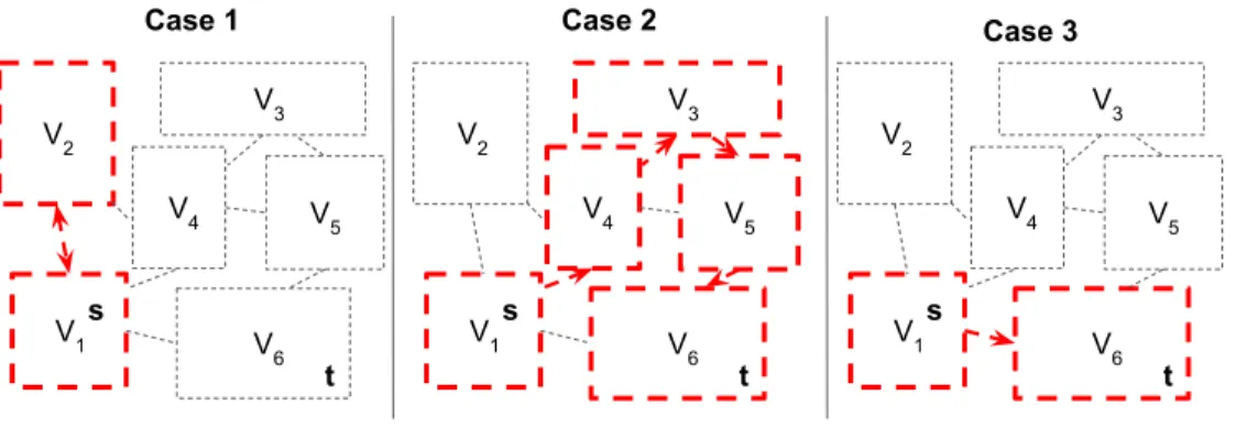
The intuition of this technique is to offer a direct passage that goes across graph regions that are likely to satisfy attribute constraints from s to t so that t can be reached faster. For example, in Figure4.3,G is partitioned into 6 regions (V1, V2, ..., V6) and suppose s and

t are in V1 and V6. If there are a lot of paths that satisfy attribute constraint from s to t,

we do not want to:

V_{1 V} 6 V₃ V₂ V₅ V₄ V_{1 V} 6 V₃ V₂ V₅ V₄ Case 1 Case 2 s t s t V_{1 V} 6 V₃ V₂ V₅ V₄ Case 3 s t

Figure 4.3: Choice of Path from s to t

• choose a long path to reach t such as a path that passes throughV1 →V4 →V3 →V5 →

V6 (case 2);

instead, we want to find a short path from s to t (e.g. case 3 V1 → V6). Our proposed

heuristic search technique is designed based on this observation. More details are presented below.

4.5.1 Index Construction for Heuristic Search

We partition the graph into clusters and build a structure called - super-graph.

Definition 17. [Super-graph]Gs is an undirected graph with super-vertex and super-edge,

and for every super-vertex and super-edge, there is a synopsis that represents the distribution of attributes in the super-vertex or super-edge.

Definition 18. [Super-vertex] Vi is a vertex in Gs such that for every vertex v in G, v

belongs to only one Vi in Gs.

∀v ∈G, v ∈Vi∧v /∈Vj if i6=j, where Vi, Vj ∈Gs

Definition 19. [Super-edge] Ei is an edge in Gs such that if there exists an edge e(u,v) between vertex u, v in G and u, v belong to two different super-vertices Vi, Vj in Gs, e(u,v) belongs to E(Vi,Vj) in Gs.

For example, in Figure 1, the social network is partitioned into 6 clusters/super-vertices. Dotted rectangles are super-vertices. There is a super-edge betweenV1 andV2 as there is an

edge froms tov6.

When building the super-graph, any clustering algorithm that fits dataset property can be used. For each vertex Vi and edge E(Vi,Vj) inGs, we build synopsis, which represents the

distribution of attributes in the super-vertex or super-edge. A simple synopsis can be a set of sample attributes drawn from vertices in the super-vertex.

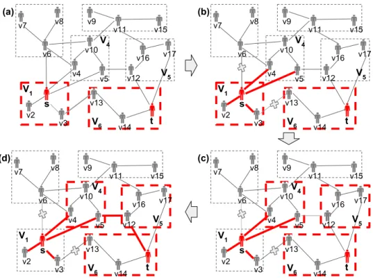
4.5.2 Efficient Query Algorithm

Algorithm 3 is the pseudo code for the query algorithm. Given s, t, Cv, Gh, and Gs (line

1), the query algorithm answers the attribute constraint reachability query. A queue q is maintained in the algorithm (line 2). In the beginning, s is put into the queue q (line 3). When the graph traversal starts, the first element v is pop from q (line 5). Then, the algorithm finds a super-graph shortest pathSPsfrom super-vertexSN[v.f irst] that contains v to super-vertex SN[t] that contains t (line 9). A guided BF Sg is performed starting at

vertex v (line 10). If a vertex vout that is not in SPs is visited, the vertex is put into q

and adjacent vertices of vout are not visited in this guided BF Sg. During graph traversal,

synopsis in super-vertex and super-edge are updated. Iftis not found inBF Sg, afterBF Sg,

another element is pop from q and the same steps as above are performed untilq is empty (line 4). Figure 4.4 is an example.

4.5.2.1 Super-graph Shortest Path GivenGs and synopsis of every super-vertex and

super-edge in Gs, the query algorithm tries to find a shortest path in Gs from super-vertex SN[s] or SN[h] that contains s or any h to super-vertex SN[t] that contains t based on the sum of estimated pass-through probability SPcost, which can be estimated by using the

attribute constraints and the synopsis.

4.5.2.2 Guided Search Basically, any graph traversal algorithm can be adopted (e.g. A∗, BF S, DF S). For simplicity, we use BFS as an example. Guided BF Sg is a modified

Algorithm 3 Efficient Query Algorithm

1: procedure ReachabilityQuery(s, t, Cv, Gh, Gs) 2: Queue q

3: q.put(pair(s, φ)) .No need to check constraint of s 4: while q.empty() = f alsedo

5: v =q.pop()

6: if visited[v.f irst] =true then

7: continue . OtherBF Sg may set visitedto true

8: end if

9: visited[v.f irst]←true

10: SPs←SGraphSP(SN[v.f irst], v.second, SN[t], G.Gs, Cv) 11: (R, q)←BF Sg(v.f irst, t, Gh, Cv, SPs, q) 12: if R=true then 13: return yes 14: end if 15: end while 16: return no 17: end procedure

v2 v3 v5 v4 v10 v13 v12 v6 v14 v9 v11 v16 v17 v15 s t v2 v3 v5 v4 v10 v13 v12 v6 v14 v7 v8 v9 _v11 v16 v17 v15 s t v2 v3 v5 v4 v10 v13 v12 v6 v14 v7 v8 v9 _v11 v16 v17 v15 s t v2 v3 v5 v4 v10 v13 v12 v6 v14 v7 v8 v9 _v11 v16 v17 v15 s t V₁ V₆ V₁ V₆ V₁ V₆ V₁ V₆ V₄ V₅ V₄ V₅ V₄ V₅ V₄ V₅ (a) (b) (c) (d) v8 v7

Figure 4.4: Example for Efficient Query Algorithm

version of typical BF S. Algorithm 4 is the pseudo code. The difference between guided BF Sg and typical BF S is that:

• vertex constraint is verified and synopsis is updated,

• vertices that are not inSPsare not traversed (line 10) and are put into a queueqGoffered

by the caller of the guided BFS (line 16), and • Es

(SN[cur],SN[v0_]), which is a super-edge that can be ignored in SGraphSP() whenSN[v0] is used as source, is put into qG together with v0.

Algorithm 4 Guided BFS

1: procedure BF Sg(cur, t, Gh, Cv, SPs, qG) 2: Queue q

3: q.put(cur)

4: while q.empty() = f alsedo

5: v =q.pop()

6: if v =t then

7: return (true, qG)

8: end if

9: if visited[v] =true then

10: continue

11: end if

12: if SN[v]∈SPs then 13: visited[v]←true

14: for all v0 ∈v.adjList do

15: if CheckConstraintBF Sg(v0, Gh, Cv) =true then 16: q.put(v0)

17: end if

18: end for

19: else . ignore E(SN[cur],SN[v0_]) inSGraphSP()

20: qG.put(pair(v, E(SN[cur],SN[v0_])))

21: end if

22: end while

23: return (f alse, qG) 24: