Received 15 May 2015 Accepted 28 June 2016
New approach to Forecasting Agro-based statistical models
Muhammad Akram
Department of Epidemiology and preventive Medicine, Monash University, The Alfred centre, Melbourne, Victoria-3004, Australia
M. Ishaq Bhatti
Department of Economics and Finance, LaTrobe University Melbourne, Victoria-3086, Australia
Muhammad Ashfaq
Institute of Agricultural and Resource Economincs University of Agriculture, Faisalabad, Pakistan
Asif Ali Khan
Office of Research, Innovation and Commercialization, University of Agriculture, Faisalabad, Pakistan
This paper uses various forecasting methods to forecast future crop production levels using time series data for four major crops in Pakistan: wheat, rice, cotton and pulses. These different forecasting methods are then assessed based on their out-of-sample forecast accuracies. We empirically compare three methods: Box-Jenkins’ ARIMA, Dynamic Linear Models (DLM) and exponential smoothing. The best forecasting models are selected from each of the methods by applying them to various agricultural time series in order to demonstrate the usefulness of the models and the differences between them in an actual application. The forecasts obtained from the best selected exponential smoothing models are then compared with those obtained from the best selected classical Box-Jenkins ARIMA models and DLMs using various forecast accuracy measures.
Keywords: forecast; exponential smoothing; ARIMA; dynamic linear model; forecast accuracy measure. 2000 Mathematics Subject Classification: 62M10, 37M10
1. Introduction
The ultimate objective of any forecasting method, such as ES or ARIMA, is to provide precise future predictions. Many new forecasting methods have become available over the last few decades,
and researchers and practitioners use various different sets of methods to conduct their empirical forecasting comparisons. For example, the major finding of [16], and [14], who used thousands of time series, was that simple methods, such as simple exponential smoothing and damped trend methods perform as well or in many cases better than those that are more statistically sophisticated ones like ARIMA models. The flexibility of exponential smoothing is demonstrated by its ability to provide forecasts for the complete taxonomy of [19], as extended by [11] and [22].
It is important to evaluate forecast accuracy using genuine forecasts. That is, it is invalid to look at how well a model fits the historical data; the accuracy of forecasts can only be determined by considering how well a model performs on new data that were not used when fitting the model. When choosing models, it is common to use a portion of the available data for fitting, and use the rest of the data (out-of-sample data) for testing the model [11]. Then the testing data can be used to measure how well the model is likely to forecast on new data.
The aim of this paper is to assess different forecasting methods based on their out-of-sample forecast accuracies. We compare various methods, such as Box-Jenkins’ ARIMA technique, dynamic linear models [20], and the exponential smoothing method, by applying them to some real time series data in order to demonstrate the differences between the models in an actual application. The rest of the paper is arranged as follows.
A brief theoretical background of various forecasting methods is given in Section 2. The various forecast accuracy measures are defined in Section 3. The three methods under discussion are then compared by applying them to various agricultural production time series in Section 4. The final section contains concluding remarks.
2. Theoretical background 2.1. Exponential Smoothing
Exponential smoothing (ES) methods, that were first proposed in the late 1950s [4], have since been among the most widely used forecasting procedures in industry and commerce, particularly in pro-duction planning, inventory control, sales forecasting, propro-duction scheduling and operations man-agement. There are a variety of methods that fall into the ES family, each having the property that forecasts are weighted combinations of past observations. That is, forecasts produced using expo-nential smoothing methods are weighted averages of past observations, with the weights decaying exponentially as the observations get older. In other words, the more recent the observation the higher the associated weight.
ES can be applied to time series data, either for smoothing the data or for producing forecasts. The basic idea behind ES is to construct an exponentially weighted moving average (EWMA) for each component of the time series, namely the level, trend and seasonality. The weight and length of each component are determined through the smoothing parameters of the components, namelyα for level,β for trend andγfor seasonality (for detail, see [17]).
2.1.1. Modeling framework
The state space framework offers a statistical rationale in support of the ES models, that are based on capturing and smoothing the existing structural components of a time series, namely the level, trend and seasonality. The framework involves 30 different models (15 with additive errors and 15 with multiplicative errors). Each model consists of a measurement equation that describes the observed
data and some transition equations that describe how the unobserved components or states (level, trend, seasonal) change over time. Hence these are referred to as state space models. Each model is denoted by its error, trend and seasonal components, following the procedure of [10], in order to allow for easy cross-referencing of the models. They code any exponential smoothing model as a triplet ETS (error, trend, seasonality). The following shorthand is used: N for none, A for additive, Adfor additive damped, M for multiplicative and Mdfor multiplicative damped. For example, AAN
refers to a model with additive errors, additive trend and no seasonality. Model ANN gives forecasts that are equivalent to simple exponential smoothing, model AAN underlies Holt’s linear method, and the additive Holt-Winters’ method is obtained by AAA. Table 1, taken from [11], shows the 15 models with additive errors.
Table 1. Models with additive errors in modelling framework Seasonal Component
Trend N A M
Component (None) (Additive) (Multiplicative)
N (None) NN NA NM
A (Additive) AN AA AM
Ad (Additive damped) Ad N AdA AdM
M (Multiplicative) MN MA MM
Md (Multiplicative damped) MdN MdA Md M
2.1.2. State space models
The state space models enable easy calculations of the likelihood, and provide facilities for the computation of prediction intervals for each model. For each of their methods, [11] proposed two state space models with a single source of error, following the general approach of [18]. The two state space formulations correspond to the additive error and multiplicative error cases, and give equivalent point forecasts but different prediction intervals and likelihoods. The general framework, given by [18], involves a state vectorxt and state space equations of the form
yt =h(xt−1) +k(xt−1)εt (2.1)
xt = f(xt−1) +g(xt−1)εt, (2.2)
where{εt}is a Gaussian white noise process with mean zero and varianceσ2. Defineet=k(xt−1)εt
andµt =h(xt−1); then,yt =µt+et. The model with additive errors is written as yt =µt+εt, so,
in this case,k(xt−1) =1. The model with multiplicative errors is written asyt =µt(1+εt). Thus,
k(xt−1) =µt for this model andεt =et/µt = (yt−µt)/µt, and hence,εt is a relative error for the
multiplicative model.
Equation (2.1) is called the measurement equation, and equation (2.2) is known as the transition equation. The termh(xt−1)describes the effect of the past onyt. The term f(xt−1)shows the effect
of the past on the current statext. The termg(xt−1)εt shows the unpredictable change inxt, and the
vectorg determines the extent of the effect of the innovation on the state. All of the exponential smoothing methods of [11] can be written in the form of equations (2.1) and (2.2). The underlying equations are given in ( [10], Table 2.2 & 2.3). The only difference between the additive error
and multiplicative error models is in the observation equation (2.1): multiplicative error models are obtained by replacingεt in additive error models withµtεt.
ES methods are arguably the most widely applied forecasting methods. They can also be regarded as a sub-case of the ARIMA framework ( [3]), but they are often preferred to ARIMA models due to their simplicity, robustness and accuracy. However, [11] showed that ES is in fact a general class of state space models that can provide optimal forecasts for a broader set of cases than ARIMA. In the opposite direction, an ARIMA model can also be put in the form of a linear state space model. The ES method has the advantage that its algorithm can be implemented relatively easily in a matrix language such as R [21] and/or ’Matlab’. This algorithm is implemented in the R packageforecast[7].
2.2. Box-Jenkins ARIMA models
ARIMA models provide another approach to time series forecasting. ARIMA is an acronym for AutoRegressive Integrated Moving Average model (integration in this context is the reverse of dif-ferencing). Exponential smoothing and ARIMA models are the two most widely-used approaches to time series forecasting, and provide complementary approaches to the problem. While exponential smoothing models were based on a description of trend and seasonality in the data, ARIMA models aim to describe the autocorrelations in the data. Since a vast literature on ARIMA methodology is available (see for example [3]), we provide a brief description here.
2.2.1. Autoregressive models
In a multiple regression model, we forecast the variable of interest using a linear combination of predictors. In an autoregression model, we forecast the variable of interest using a linear combina-tion of past values of the variable. The term autoregression indicates that it is a regression of the variable against itself. Thus an autoregressive model of order pcan be written as
yt=c+ϕ1yt−1+ϕ2yt−2+···+ϕpyt−p+et,
wherecis a constant andet is white noise. This is like a multiple regression but with lagged values
ofyt as predictors. We refer to this as an AR(p) model.
2.2.2. Moving average models
Rather than use past values of the forecast variable in a regression, a moving average model uses past forecast errors in a regression-like model.
yt=c+et+θ1et−1+θ2et−2+···+θqet−q,
whereetis white noise. We refer to this as an MA(q) model. Of course, we do not observe the values
ofet, so it is not really regression in the usual sense.
2.2.3. Non-seasonal ARIMA models
If we combine differencing with autoregression and a moving average model, we obtain a non-seasonal ARIMA model. The full model can be written as
whereyt′is the differenced series (it may have been differenced more than once). The “predictors” on the right hand side include both lagged values ofytand lagged errors. We call this an ARIMA(p,d,q)
model. Once we start combining components in this way to form more complicated models, it is much easier to work with the backshift notation. Then equation (2.3) can be written as
(1−ϕ1B− ··· −ϕpBp)(1−B)dyt =c+ (1+θ1B+···+θqBq)et
whereBpyt =yt−p. Selecting appropriate values forp, dandqcan be difficult. Theauto.arima()
function in R will do it automatically. This algorithm is also implemented in the R packageforecast. Theauto.arima()function in R uses a variation of the [8] algorithm that combines unit root tests, minimization of the AICc and MLE to obtain an ARIMA model.
The order of ARIMA model (i.e., the values of p,d andq) is determined by Akaike’s Infor-mation Criterion (AIC). The algorithm set upper bound on the order pandq at 5, as it is almost impracticable to have the order porqmore than 5. Once the model order has been identified, we need to estimate the parametersc,ϕ1,···,ϕp,θ1,···,θqby MLE. See [3] for detail.
2.3. Dynamic linear models
In recent decades, dynamic linear models, and state space models more generally, have increasingly become a focus of interest in time series analysis. Dynamic linear models (DLM) represent a special case of general state space models, being linear and Gaussian. These models are specified by means of two equations:
yt =Htxt+εt (2.4)
xt =Ftxt−1+ηt, (2.5)
whereεt∼N(0,σε2)andηt ∼N(0,ση2)are two independent white noise sequences,yt denotes the
observation at timet, andxtis the random vector ofkunobservable states of the system at timet.Ht
is a fixed vector andFt is a fixed state matrix. The usual features of a time series, such as trend and
seasonality, can be modeled within this format. Sometimes,HandFare assumed to be independent oft, in which case the model is a time series DLM. [10] refer to such time series DLMs as multi disturbance or multiple source of error (MSOE) state space models, as the equations (2.4) and (2.5) have two independent source of errors,εt andηt.
When ηt =gεt (where g is a fixed vector of persistence parameters), the MSOE state space
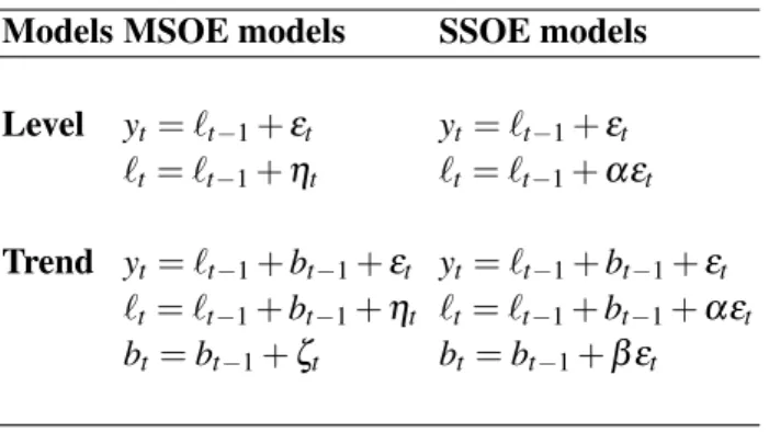
model becomes equivalent to the single source of error (SSOE) state space model introduced in Section 2.1.2. Table 2 (taken from [10]) shows the corresponding standard structural models from the two approaches for the local level and linear trend models. Note that although the common symbolsℓ,bandεare used to represent the level, slope and innovation respectively, their meanings differ between the two frameworks.
It is possible to represent an ARIMA model, whether univariate or multivariate, as a DLM (see Chapter 3 of [20]). However, in spite of the fact that an ARIMA model can formally be considered a DLM, the philosophies underlying the two classes of models are quite different: on the one hand, ARIMA models provide a black-box approach to data analysis, offering the possibility of forecast-ing future observations, but with a very limited interpretability of the fitted model; on the other hand, the DLM framework encourages the analyst to think in terms of easily interpretable, albeit unobservable, processes — such as trend and seasonal components — that drive the observed time series (for details, see Chapter 3 of [20]).
Table 2. Comparison of local level and local linear trend models Models MSOE models SSOE models Level yt=ℓt−1+εt yt=ℓt−1+εt
ℓt =ℓt−1+ηt ℓt =ℓt−1+αεt
Trend yt=ℓt−1+bt−1+εt yt=ℓt−1+bt−1+εt
ℓt =ℓt−1+bt−1+ηt ℓt =ℓt−1+bt−1+αεt
bt =bt−1+ζt bt=bt−1+βεt
For DLM, estimation and forecasting can be obtained recursively by the well known Kalman filter [12]. This opens the way for estimation of any unknown parameter in the model (see for detail [6]). The R functionStructT Sin the R packagestatsis used to fit DLM. It uses the Kalman filter to implement the maximum likelihood approach to develop the estimates. Since all the data series considered are non-seasonal, therefore it selects the best model among non-seasonal DLM using AIC.
3. Measures of forecast accuracy
In the past, many studies have been conducted with the aim of identifying which method will pro-vide the most accurate forecasts for a given class of time series data. In this section, the error mea-sures used for drawing conclusions about the relative accuracies of models’ forecast performances are discussed.
The Mean Square Error (MSE) is often used to compare the performances of forecasting models because of its computational convenience and theoretical relevance to statistics. However, it is scale-dependent, and so should not be used to compare different series. The most widely used unit-free measure is the Mean Absolute Percentage Error (MAPE), and many books recommend its use (see [2, 5]). However, one disadvantage of the MAPE is that it is relevant only for ratio-scaled data (i.e., data with a meaningful zero). [1] recommended the Median Relative Absolute Error (MdRAE) when few series are available, and the Median Absolute Percentage Error (MdAPE) otherwise. [15] discussed some problems with the RAE, and proposed an alternative measure called Symmetric Mean Absolute Percentage Error (sMAPE), a modification of the MAPE. [1] referred to this as the Unbiased Absolute Percentage Error (UAPE). However, [13] later commented on the sMAPE measure and showed that it actually penalizes low forecasts more than high forecasts, meaning that a more accurate name would be the MeanAsymmetricAbsolute Percentage Error.
[9] proposed a new measure called the Mean Absolute Scaled Error (MASE), that is suitable for all three of the scenarios described earlier, and involves scaling the error based on the in-sample mean absolute error (MAE) from the na¨ıve forecast method.
With so many measures of the forecast accuracy available, it is difficult to choose the most suitable one. In this paper, the following three commonly used forecast accuracy measures have been used to analyze the performances of the forecasts by applying them when forecasting the various time series.
(i) Root Mean Squared Error (RMSE) (ii) Mean Absolute Percentage Error (MAPE) (iii) Mean Absolute Scaled Error (MASE)
These particular measures are chosen because several authors and practitioners believe that they are more reliable and sensitive to small changes than others (see [9]). Short descriptions of these accuracy measures are given below.
(i) RMSE
The root mean squared error (RMSE) is defined as follows: RMSE= √ 1 n n
∑
t=1 (Yt−Ft)2,whereYt is the observed value,Ft is the forecast (predicted) value at timet, andnis the length of
the data series. (ii) MAPE
First, a relative or percentage error is defined as PEt= (Y t−Ft Yt ) ×100,
whereYt is the actual value andFt is the forecast value at timet. Then, the MAPE is defined as the
average of the absolute values of PE, as follows (for more details, see Makridakis et al., 1998): MAPE=1 n n
∑
t=1 |PEt|. (iii) MASE[9] proposed a new but related idea that is suitable for all three of the scenarios described earlier. This scaled error is defined as
qt= Yt−Ft 1 n−1∑ n i=2|Yi−Yi−1| , (3.1)
which is clearly independent of the scale of the data. A scaled error is less than one if it arises from a better forecast than the average one-step na¨ıve forecast computed in-sample. Conversely, it is greater than one if the forecast is worse than the average one-step na¨ıve forecast computed in-sample. The Mean Absolute Scaled Error (MASE) is simply
MASE=mean(|qt|).
Thein-samplemean absolute error (MAE) is used in the denominator as it is always available and effectively scales the errors. In contrast, the out-of-sample MAE for the na¨ıve method can be based on very few observations and is therefore more variable. The only situation in which these measures would be infinite or undefined is when all historical observations are equal.
4. Empirical analysis
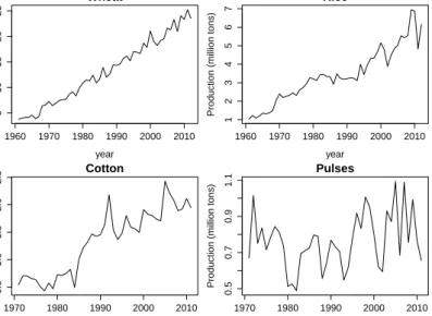
In this section, the exponential smoothing method, the dynamic linear model and the Box-Jenkins method are applied to some real agriculture time series data in order to demonstrate the differences between the methods/models in an application. The time series used are wheat production (WP), rice production (RP), cotton production (CP) and pulses production (PP). All of the data sets are annual, covering the period 1961 to 2012 for wheat and rice, and the period 1971 to 2011 for cotton and pulses. The data have been collected from various issues of the Agricultural Statistics of Pakistan, published by the Ministry of Food and Agriculture (Economic Wing), government of Pakistan, and Pakistan Economic Surveys, published by the Economic Advisor wing, Finance Division, government of Pakistan. The time series are plotted in Figure 1.
Wheat
year
Production (million tons)
1960 1970 1980 1990 2000 2010 5 10 15 20 25 Rice year
Production (million tons)
1960 1970 1980 1990 2000 2010 1 2 3 4 5 6 7 Cotton year
Production (million tons)
1970 1980 1990 2000 2010 0.5 1.0 1.5 2.0 2.5 Pulses year
Production (million tons)
1970 1980 1990 2000 2010
0.5
0.7
0.9
1.1
Fig. 1. Time series data
Agriculture is the backbone of the Pakistan’s economy, and plays an important role in the bet-terment of the large proportion of the population that live in rural areas in particular, and the overall economy in general. The growing population of Pakistan is a real point of concern that needs to be addressed by proper and timely planning for a food supply. Regarding food grain crops, wheat and rice are the main staple foods of the people of Pakistan, as well as being the most important parts of the agriculture sector.
To enable a forecast comparison, each of the time series (Figure 1) is divided into two parts, a training set (comprising 80% of the data) and atest set(comprising 20% of the data). That is, we hold back the last 20% of the data, called the test set(we may call it future sample paths), and fit the model on the rest of the data, called thetraining set. The best selected exponential smoothing model, the best selected DLM and the best selected ARIMA model are then fitted to thetraining set using maximum likelihood estimation.
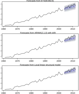
In order to compare the performances of the models, we have plotted the forecasts of wheat, rice, cotton and pulses production in Figures 2–5, respectively. Top panel: forecasts from the best selected exponential smoothing model. Middle panel: forecasts from the best selected ARIMA.
Bottom panel: forecasts from the best selected DLM model. The forecasts are based on models fitted to the data up to 2003. The dark (light) shaded region indicates 95% (80%) prediction intervals. The actual values in the forecast period are also shown. Overall, the exponential smoothing method tends to perform well, as it is generally the best (for the wheat and rice time series) or second-best (for the cotton and pulses time series) in terms of forecast accuracies, and gives more reasonable forecasts than its DLM and ARIMA counterparts. The performance of DLM is notable, as it outperforms the ARIMA method in all cases except for the pulses series. From Figure 2, it can be seen that the forecasts from the three methods all look quite similar, underestimating the actual values of wheat production. However, the measures of forecasting accuracy (see Table 3) suggest that the exponential smoothing method performs better than its counterparts. Moreover, the actual values in the forecast period are well within the 95% prediction intervals obtained via exponential smoothing.
Forecasts from ETS(M,Md,N)
million tones 1960 1970 1980 1990 2000 2010 5 10 15 20 25
Forecasts from ARIMA(2,1,0) with drift
million tones 1960 1970 1980 1990 2000 2010 5 10 15 20 25
Forecasts from Local linear structural model
million tones 1960 1970 1980 1990 2000 2010 5 10 15 20 25
Fig. 2. Historical data (solid line) and forecasts (dashed line) for thewheat productiontime series.
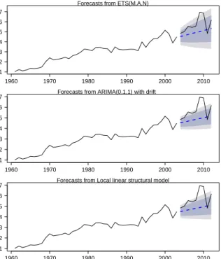
The forecasts and prediction intervals produced by the three methods for the rice time series are shown in Figure 3. The forecasts obtained from the various methods look quite different; in partic-ular, the prediction intervals are much wider in the case of exponential smoothing than for the other methods. This is because the prediction intervals produced by ES reflect the uncertainty associated with the data set, especially at the end of the training set, while the ARIMA and DLM methods seem to fail to pick it up properly. Furthermore, according to the forecast accuracy measures, the ES method again performs well relative to the other techniques for the rice time series data (see Table 3).
Figure 4 shows that the ES and ARIMA methods are both unable to produce very good forecasts for the cotton time series relative to the DLM, which seems to pick up some form of a trend from thetraining set. According to the forecast accuracy measures, the DLM takes the lead for the cotton
Forecasts from ETS(M,A,N) million tones 1960 1970 1980 1990 2000 2010 1 2 3 4 5 6 7
Forecasts from ARIMA(0,1,1) with drift
million tones 1960 1970 1980 1990 2000 2010 1 2 3 4 5 6 7
Forecasts from Local linear structural model
million tones 1960 1970 1980 1990 2000 2010 1 2 3 4 5 6 7
Fig. 3. Historical data (solid line) and forecasts (dashed line) for therice productiontime series.
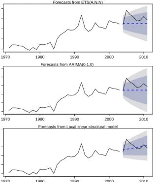
time series, although the exponential smoothing method again beats the Box-Jenkins ARIMA tech-nique. Only for the pulses production data (Figure 5), where strong stationarity is very prominent, the Box-Jenkins ARIMA technique perform better than the other methods, with ES again standing second-best.
The various measures of forecast accuracy, namely the root mean squared error (RMSE), mean absolute percentage error (MAPE) and mean absolute scaled error (MASE), have also been cal-culated for all data sets over the forecast period (test set or future sample paths) for each model. According to these accuracy measures (Table 3), the exponential smoothing method comes out as the best for the wheat and rice time series, and second-best for the cotton and pulses time series. The DLM performs best for the cotton time series, while the Box-Jenkins ARIMA technique is best for the pulses time series, where strong stationarity is very prominent. While these are only few empirical examples, making it hard to draw general conclusions, the evidence is consistent with Figures 2 to 5 in suggesting that the exponential smoothing method performs better than either the DLM or Box-Jenkins ARIMA method.
5. Conclusions
The main objective of any forecasting method is to make precise predictions of future random events. This paper has assessed different forecasting methods based on their out-of-sample fore-cast accuracy measures. Three methods, Box-Jenkins’ ARIMA, exponential smoothing (ES) and dynamic linear models (DLM), have been used to produce predictions for four important crops in Pakistan, that play important roles in Pakistan’s economy.
Forecasts from ETS(A,N,N) million tones 1970 1980 1990 2000 2010 0.5 1.0 1.5 2.0 2.5
Forecasts from ARIMA(0,1,0)
million tones 1970 1980 1990 2000 2010 0.5 1.0 1.5 2.0 2.5 3.0
Forecasts from Local linear structural model
million tones 1970 1980 1990 2000 2010 0.5 1.0 1.5 2.0 2.5 3.0
Fig. 4. Historical data (solid line) and forecasts (dashed line) for thecotton productiontime series.
Forecasts from ETS(M,N,N)
million tones 1970 1980 1990 2000 2010 0.5 0.6 0.7 0.8 0.9 1.0 1.1
Forecasts from ARIMA(1,0,0) with non−zero mean
million tones 1970 1980 1990 2000 2010 0.5 0.6 0.7 0.8 0.9 1.0
Forecasts from Local linear structural model
million tones 1970 1980 1990 2000 2010 0.2 0.4 0.6 0.8 1.0 1.2 1.4 1.6
Table 3. Measures of forecast accuracy for each model
Measure Method Wheat Rice Cotton Pulses
MASE ES 1.302 3.472 1.759 1.285 ARIMA 1.797 3.678 1.864 1.245 DLM 1.308 3.788 1.138 1.356 MAPE ES 5.004 14.062 13.544 16.030 ARIMA 6.830 14.825 14.352 14.902 DLM 5.026 15.264 8.749 18.914 RMSE ES 1366 1018 347 182 ARIMA 1913 1086 366 193 DLM 1374 1119 248 173
Empirical comparisons have been performed using various different forecast accuracy measures, which have suggested that the exponential smoothing method performs better (either best or second-best in terms of the forecast accuracy measures) than its competitors, the DLM and the Box-Jenkins ARIMA. The DLM performs best for the cotton time series, followed by ES, while ARIMA does better for pulses, followed by ES. These forecasts may be helpful in determining prices of these four commodities in advance for the farmers and financial institutions.
References
[1] J. S. Armstrong and F Collopy, Error measures for generalizing about forecasting methods: empirical comparison,International Journal of Forecasting08(1992) 69-80.
[2] B.L. Bowerman, R.T. OConnell and A.B. Koehler,Forecasting, time series and regression: an applied approach, (Thomson Brooks/Cole, Belmont CA, 2004).
[3] G.E.P. Box, G. Jenkins and G.C. Reinsel,Time series analysis: forecasting and control, 4th Ed (Hobo-ken, N.J. : John Wiley, 2008).
[4] R.G. Brown,Statistical forecasting for inventory control, 4th edn (McGraw-Hill, New York, 1959). [5] J.E. Hanke and A.G. Reitsch, Business forecasting, 5th edn (Prentice-Hall: Englewood Cliffs, NJ,
1995).
[6] A.C. Harvey,Forecasting, structural time series models and the Kalman filter, (Cambridge University Press, Cambridge, 1989).
[7] R.J. Hyndman, G. Athanasopoulos, S. Razbash, D. Schmidt, Z. Zhou and Y Khan, forecast: Fore-casting functions for time series and linear models., R package version, URL: http://CRAN.R-project.org/package=forecast4.04(2013).
[8] R.J. Hyndman, and Y Khandakar, Automatic time sereis forecasting: the forecast package for r,Journal of Statistical Software27(3)(2008).
[9] R.J. Hyndman, and A.B. Koehler, Another look at measures of forecast accuracy,International Journal of Forecasting22(4)(2006) 679–688.
[10] R.J. Hyndman, A.B. Koehler, J.K. Ord and R.D. Snyder,Forecasting with exponential smoothing: The state space approach, (Springer-Verlag: Berlin Heidelberg, 2008).
[11] R.J. Hyndman, A.B. Koehler, R.D. Snyder and S. Grose, A state space framework for automatic fore-casting using exponential smoothing methods,International Journal of Forecasting18(3)(2002) 439– 454.
[12] R.E. Kalman, A new approach to linear filtering and prediction problems,Journal of Basic Engineering (Series D)82(1)(1960) 35–45.
[13] R.E. Kalman, The asymmetry of the sAPE measure and other comments on the M3-competition, Inter-national Journal of Forecasting17(2001) 537–584.
[14] S. Makridakis and M. Hibon, The M3-competition: results, conclusions and implications,International Journal of Forecasting16(2000) 451–476.
[15] S. Makridakis, Accuracy measures: theoretical and practical concerns,International Journal of Fore-casting9(1993) 527–529.
[16] S. Makridakis, A. Anderson, R.Carbone, R. Fildes, M. Hibon, R.L.J. Newton, E. Parzen and R. Winkler, The accuracy of extrapolation (time series) methods: results of a forecasting competition,Journal of Forecasting1(1982) 111–153.
[17] S. Makridakis, S.C. Wheelwright and R.J. Hyndman,Forecasting: methods and applications, 3rd edn (John Wiley and Sons, New York, 1998).
[18] J.K. Ord, A.B. Koehler and R.D. Snyder, Estimation and prediction for a class of dynamic nonlinear statistical models,Journal of American Statistical Association92(1997) 1621–1629.
[19] C.C. Pegels, Exponential smoothing: some new variations,Management Science12(1969) 311–315. [20] G. Petris, S. Petrone and R. Campagnoli,Dynamic Linear Models with R, (Springer, 2009).
[21] R Core Team (2013), R: A Language and Environment for Statistical Computing, R Foundation for Statistical Computing, (Vienna, Austria, URL: http://www.R-project.org/, 2009).
[22] J.W. Taylor, Exponential smothing with damped multiplicative trend, International Journal of Fore-casting19(2003) 715–725.