Department of Mathematics
Uncertainty quantification for spatial
field data using expensive computer
models: refocussed Bayesian calibration
with optimal projection
James Martin Salter
March 2017
Supervised by
Daniel Williamson
Peter Challenor
Submitted by James Martin Salter, to the University of Exeter as a thesis for the degree of Doctor of Philosophy in Mathematics , March 2017.
This thesis is available for Library use on the understanding that it is copyright material and that no quotation from the thesis may be published without proper acknowledgement.
I certify that all material in this thesis which is not my own work has been identi-fied and that no material has previously been submitted and approved for the award of a degree by this or any other University.
In this thesis, we present novel methodology for emulating and calibrating computer mod-els with high-dimensional output.
Computer models for complex physical systems, such as climate, are typically expensive and time-consuming to run. Due to this inability to run computer models efficiently, statistical models (‘emulators’) are used as fast approximations of the computer model, fitted based on a small number of runs of the expensive model, allowing more of the input parameter space to be explored. Common choices for emulators are regressions and Gaussian processes.
The input parameters of the computer model that lead to output most consistent with the observations of the real-world system are generally unknown, hence computer models require careful tuning. Bayesian calibration and history matching are two methods that can be combined with emulators to search for the best input parameter setting of the computer model (calibration), or remove regions of parameter space unlikely to give output consistent with the observations, if the computer model were to be run at these settings (history matching). When calibrating computer models, it has been argued that fitting regression emulators is sufficient, due to the large, sparsely-sampled input space. We examine this for a range of examples with different features and input dimensions, and find that fitting a correlated residual term in the emulator is beneficial, in terms of more accurately removing regions of the input space, and identifying parameter settings that give output consistent with the observations. We demonstrate and advocate for multi-wave history matching followed by calibration for tuning.
In order to emulate computer models with large spatial output, projection onto a low-dimensional basis is commonly used. The standard accepted method for selecting a basis is to usenruns of the computer model to compute principal components via the singular
lated. We show that when then runs used to define the basis do not contain important patterns found in the real-world observations of the spatial field, linear combinations of the SVD basis vectors will not generally be able to represent these observations. Therefore, the results of a calibration exercise are meaningless, as we converge to incorrect parameter settings, likely assigning zero posterior probability to the correct region of input space. We show that the inadequacy of the SVD basis is very common and present in every climate model field we looked at.
We develop a method for combining important patterns from the observations with signal from the model runs, developing a calibration-optimal rotation of the SVD basis that allows a search of the output space for fields consistent with the observations. We illustrate this method by performing two iterations of history matching on a climate model, CanAM4. We develop a method for beginning to assess model discrepancy for climate models, where modellers would first like to see whether the model can achieve certain accuracy, before allowing specific model structural errors to be accounted for.
We show that calibrating using the basis coefficients often leads to poor results, with fields consistent with the observations ruled out in history matching. We develop a method for adjusting for basis projection when history matching, so that an efficient and more accurate implausibility bound can be derived that is consistent with history matching using the computationally prohibitive spatial field.
throughout, and for convincing me to do a PhD in the first place!
Thanks also to Peter Challenor for many interesting discussions.
Thanks to those at CCCMA that allowed us to run an ensemble on
their supercomputer.
Finally, a huge thank you to my family and friends, without whom
none of this would have been possible.
List of tables 11
List of figures 12
Publications 21
1 Introduction 23
1.1 Aims . . . 25
1.2 Structure of the thesis . . . 26
2 Literature review 29 2.1 Computer models . . . 29 2.2 Uncertainty quantification . . . 30 2.3 Emulation . . . 31 2.3.1 Gaussian processes . . . 32 Correlation functions . . . 33
The nugget parameter . . . 35
Fitting a Gaussian process emulator . . . 36
Estimating parameters . . . 38
2.3.2 Bayes linear methods . . . 40
2.4 Multivariate emulation . . . 41
2.4.1 Basis methods . . . 46
2.5 Bayesian calibration . . . 52
2.5.1 Forecasting . . . 59
2.6 Calibration in higher dimensions . . . 60
2.6.1 Choice ofΓq . . . 64
2.7 History matching . . . 65
2.7.1 Refocussing . . . 68
2.7.3 Discrepancy . . . 73
2.8 Tuning climate models . . . 75
2.8.1 Data assimilation . . . 77
3 Multi-wave emulation and calibration 79 3.1 Introduction . . . 79
3.2 Regression vs Gaussian process emulators . . . 80
3.2.1 Tractability . . . 81
3.2.2 Sparse sampling of the input space . . . 82
3.3 Simulation study design . . . 84
3.3.1 Toy examples . . . 87
3.3.2 Modelling choices . . . 88
3.3.3 Parameter estimation . . . 90
3.3.4 Validating emulators . . . 92
3.3.5 Sampling from NROY space . . . 92
3.4 Multi-wave history matching results . . . 93
3.4.1 Size of NROY space . . . 94
3.4.2 Highlighting unusual results . . . 97
3.4.3 Composition of NROY space . . . 98
3.5 Sensitivity to sample design . . . 101
3.5.1 Refitting emulators . . . 102
3.6 Application to an environmental model . . . 105
3.6.1 Summary statistics . . . 107
3.6.2 Sampling from the database . . . 108
3.6.3 True NROY space . . . 109
3.6.4 History matching results . . . 110
3.6.5 Calibration . . . 113
3.7 Discussion . . . 114
3.8 Conclusion . . . 119
4 Looking the wrong way: the problem with the SVD basis 121 4.1 Introduction . . . 121
4.2 A spatial toy example . . . 122
4.3.1 For the toy example . . . 127
4.3.2 Reconstructingz . . . 129
4.3.3 Quantifying the reconstruction error . . . 133
4.4 Calibrating the toy function . . . 137
4.4.1 Specifying the discrepancy variance . . . 138
4.4.2 True NROY space . . . 140
4.4.3 Calibration . . . 141
4.4.4 History matching on the field . . . 145
4.5 Climate models . . . 147
4.5.1 ORCA2 . . . 147
4.5.2 CCCMA model . . . 151
4.5.3 Reconstructing the CanAM4 observations . . . 153
4.6 Constructing a physical basis . . . 157
4.6.1 The residual basis . . . 158
4.6.2 Orthogonality of the basis . . . 159
4.6.3 Imposing orthogonality on a basis . . . 161
4.6.4 Proportion of ensemble variability explained . . . 163
4.7 Applications of the physical basis . . . 165
4.7.1 Using the observations in the physical basis . . . 166
4.7.2 Selecting a basis for CanAM4 . . . 169
4.8 Discussion . . . 170
4.9 Conclusion . . . 173
5 Optimal rotation of a basis 175 5.1 Introduction . . . 175 5.2 Basis rotation . . . 176 5.2.1 Rotation in ndimensions . . . 178 5.3 Optimising forΛ . . . 181 5.3.1 Invariance ofRW(B,·) to rotation . . . 182 5.3.2 Rotation as re-weighting . . . 184
5.3.3 Combining Gram-Schmidt and re-weighted basis vectors . . . 185
5.4 The iterative optimal rotation algorithm . . . 188
5.4.1 Discussion of the algorithm . . . 189
5.5 Basis rotation for the toy function . . . 194
5.5.1 Calibration with the rotated basis . . . 196
5.5.2 History matching . . . 199
5.6 Combining history matching and calibration . . . 201
5.6.1 Ensemble design . . . 202
5.6.2 Wave 2 . . . 204
5.6.3 Wave 2 calibration . . . 207
5.7 Weighted projection . . . 210
5.7.1 Non-increasing reconstruction error . . . 210
5.7.2 Weighted projection . . . 213
5.8 Refocussing continued: wave 3 . . . 215
5.8.1 History matching . . . 216
5.8.2 Bayesian calibration . . . 216
5.9 Discussion . . . 218
5.10 Conclusion . . . 222
6 Iterative history matching of CanAM4 223 6.1 Introduction . . . 223
6.2 High-dimensional calibration . . . 224
6.2.1 Coefficient implausibilities for the toy function . . . 226
6.2.2 Selecting a conservative bound for history matching . . . 229
6.2.3 ModellingIc vs If . . . 231
6.2.4 Bound for the toy function . . . 232
6.2.5 Efficiently calculating the field implausibility . . . 234
6.3 History matching a climate model . . . 236
6.3.1 Basis rotation and emulation . . . 236
CLTO . . . 237
RTMT . . . 238
TA . . . 239
6.3.2 Specifying the discrepancy . . . 240
6.3.3 Inferring the coefficient bounds . . . 243
6.3.4 NROY space . . . 245
6.3.5 Ensemble design . . . 246
6.4.1 Ensemble summary . . . 247
6.4.2 Rotating in NROY space . . . 250
6.4.3 Adding discrepancy for TA . . . 255
6.4.4 Wave 2 rotation and emulation . . . 258
6.4.5 Wave 2 history matching . . . 262
6.5 Discussion . . . 263 6.6 Conclusion . . . 267 7 Conclusion 268 7.1 Summary . . . 268 7.2 Future work . . . 270 Appendices 274 A Toy function definitions 275 A.1 1-dimensional toy functions . . . 275
A.2 Spatial toy function . . . 276
B Emulator diagnostics 278 B.1 Univariate toy functions . . . 278
B.2 IC fault model . . . 279
B.3 Spatial toy function . . . 279
B.4 CanAM4 emulators . . . 283
C Miscellaneous plots 287 C.1 Calibration traceplots . . . 287
C.2 CanAM4 plots . . . 289
D Code for emulation, rotation and spatial calibration 292 D.1 Emulation . . . 292
D.2 Basis projection and rotation . . . 301
D.3 History matching and Bayesian calibration . . . 306
D.4 Example . . . 310
3.1 Information about the toy functions for history matching. Range denotes the spread of possible outputs for the function, and NROY size denotes the theoretical size of NROY space, given this error structure. . . 88 3.2 The size of NROY space (as a percentage of the original space) after wave
4, when only regression emulators have been used, and when a Gaussian process has always been used. . . 95
6.1 The size of the NROY space at waves 1 and 2, when the field and coefficient implausibilities are each used, with the bound set as the 0.995 value of the chi-squared distribution with the associated number of degrees of freedom. The percentages in brackets indicate how much of the true NROY space is not ruled out. . . 229 6.2 A table giving the discrepancy variance for each of the fields, with the values
used in their calculation, withW=Σe from (6.6). . . 242
6.3 A table giving the standard bound that would be used based on the chi-squared distribution, and the new bound given by the implausibility model. 245 6.4 A table showing the reconstruction errors for the truncated rotated basis at
waves 1 and 2, and the discrepancy variances and history matching bounds for each field. . . 259
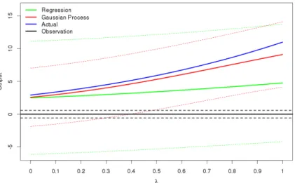
3.1 How the prediction and 99% uncertainty bounds change for a regression emulator (green) and a Gaussian process emulator (red) for a line between two design points x1, x2 in 10-dimensional space, with this line given by
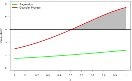
λx2+ (1−λ)x1. The blue line shows the toy function. The observation is taken to be 0, observed with an observation error given by the dotted black lines. The nugget for the Gaussian process emulator is relatively large in this example. . . 83 3.2 The implausibility I(x) for the above two emulators. With 3 chosen as
the threshold for ruling out points, the regression emulator cannot rule out anything in this part of space, while the Gaussian process emulator can for
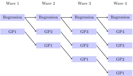
λ >0.52. . . 84 3.3 Flow chart showing the emulators built for a comparison between the
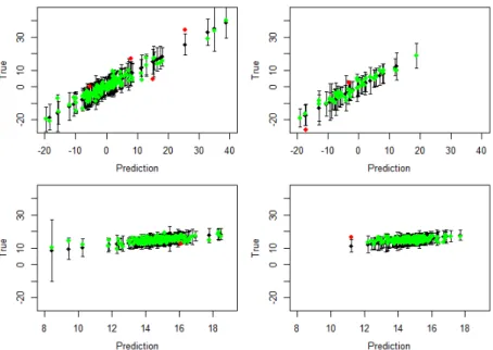
regression-only case and the Gaussian process case. GP1 denotes that a Gaussian process is used from wave 1 onwards. . . 85 3.4 Leave-one-out cross validation plots (left) and prediction for the validation
set (right), for the Gaussian process emulators for function 1, after wave 1 (top) and wave 4 (bottom). The black points indicate the prediction given by the emulator, with 95% error bars. The green and red points are the actual function values, coloured green if they lie within the 99% error bars around the prediction. Emulators are deemed to validate well if there are not too many or too few of the true values outside of these error bars. . . . 93 3.5 Top left function 1, top right function 2, bottom left function 3, bottom right
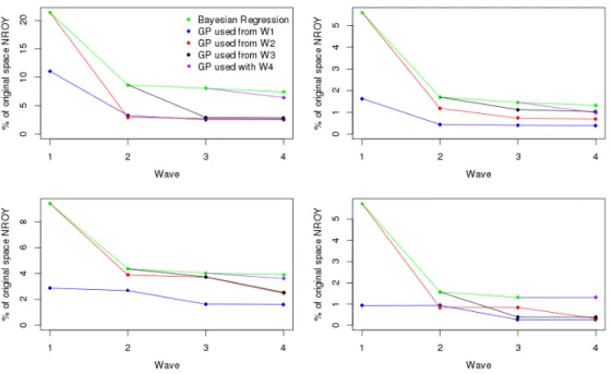
borehole function. This picture shows the sizes of NROY space at each wave when history matching each of the toy functions with regression emulators, and when a Gaussian process emulator starts to be used at different waves. 94
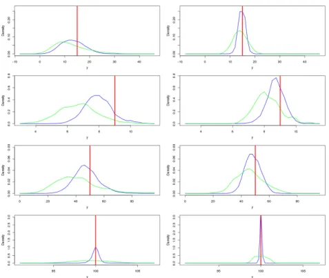
3.6 The weighted densities for the function output at points in NROY space after wave 1 (left) and wave 4 (right) for each of the four functions, for the ‘always Gaussian process’ case (blue) and the regression emulators (green). The observation for each function is given by the red line. . . 99 3.7 The progression of the sizes of NROY space for the borehole function. The
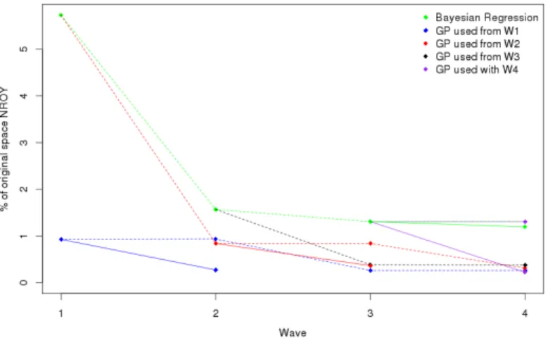
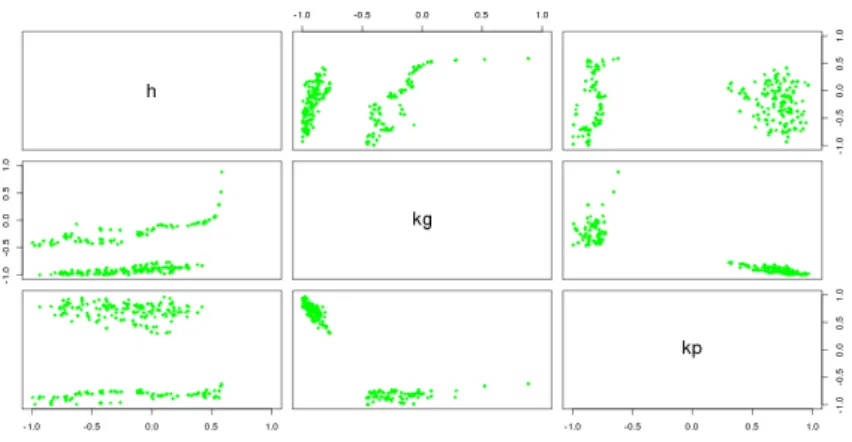
dotted lines indicate the original NROY spaces found, as in Figure 3.5, with the solid lines showing improvements achieved through either fitting a new mean function (in the case of GP2 (red line)), or by taking a new sample in the existing NROY space. . . 104 3.8 The observations for the IC fault model. . . 107 3.9 The parameter settings for the runs in the database that are in NROY space
according to the three chosen statistics. . . 109 3.10 The progression of the size of NROY space when history matching the IC
fault model with only regression emulators, and when starting to use a Gaussian process emulator at different waves. . . 110 3.11 A parameter plot showing the true NROY space (green) and points classified
as being in NROY space after 4 waves when regression emulators are used at each wave. . . 111 3.12 A parameter plot showing the true NROY space (green) and points classified
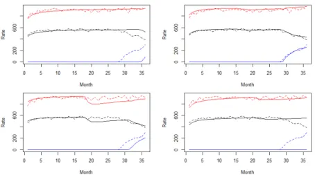
as being in NROY space after 4 waves when Gaussian process emulators are used at each wave. . . 111 3.13 The output for four runs in NROY space, when a Gaussian process emulator
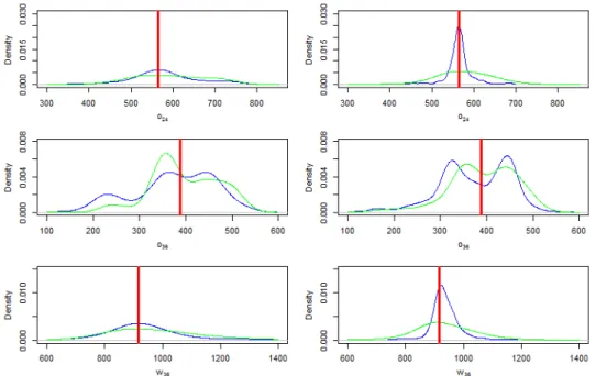
is always used, with the solid lines giving the model output for a particular parameter choice, and the dotted lines showing the observations. Red is the water injection rate, black is the oil production rate, and blue is the water cut. . . 112 3.14 The weighted densities for the function output at points in NROY space
after wave 1 (left) and wave 4 (right) for the output statistics, o24, o36 and w36, for the ‘always Gaussian process’ case (blue) and the regression emulators (green). The observation for each of the outputs is given by the red line. . . 114
4.1 The observations,z, for the toy function (left), and the mean of the ensemble F. . . 124
4.2 The first 8 SVD basis vectors of the centred ensemble. . . 128 4.3 The leave-one-out cross-validation plot for the emulator for the coefficients
given by projecting onto the sixth vector of the SVD basis, with the error bars representing 99% uncertainty bounds. . . 130 4.4 The reconstruction ofz after it has been projected onto the first four SVD
basis vectors Γ4, and the full SVD basisΓ. . . 132 4.5 A plot showing how the reconstruction error, scaled by the field sizel= 100
(red), and percentage of ensemble variability explained (blue) change as the SVD basis is increased in size, for W = Il (left) and W = 4Il. The horizontal dotted line gives=T /100. The vertical dotted line shows how many basis vectors are required to explain at least 95% of ensemble variability.136 4.6 A plot showing how the reconstruction error (red) and percentage of
en-semble variability explained (blue) change as the SVD basis is increased in size, for W=Σe+Ση, with the dotted lines defined as in Figure 4.5. As
before, the lefty-axis is scaled byl= 100. . . 140 4.7 A picture showing the true NROY space for the spatial toy function. The
density plots on the bottom left half show the proportion of space that is in the true NROY space for each pairwise combination of the parameters, averaged over the remaining parameters. The plots on the top right show the corresponding points in the true NROY space. The axes have been switched for the plots in the lower half (i.e. the higher parameter is always on the x-axis) so that these correspond to the top half. The green point corresponds to x∗. . . 141 4.8 The posterior distributions for each of the parameters, when calibration is
performed using the SVD basisΓ4. The red vertical lines indicate the true value of x∗. . . 144 4.9 f(x) at 16 samples of x from the calibration posterior distribution, using
the SVD basisΓ4 for projection and emulation. . . 145 4.10 The anomaly between the ensemble mean and the SST observations, in◦C. 148 4.11 The first nine basis vectors of the SVD basis for the centred ORCA ensemble.149
4.12 The anomaly between the reconstruction of the SST observations and the observations, using the first 10 SVD basis vectors for projection and back-projection. The right panel shows the VarMSE plot with W = 19Il (solid line) andW=Il (dotted line). . . 150 4.13 The total cloud overlap percentage (CLTO) anomaly for the standard run
of CanAM4. . . 152 4.14 The top of atmosphere (TOA) balance anomaly for the standard run of
CanAM4, in W/M2. . . 152 4.15 The vertical air temperature anomaly for the standard run of CanAM4, in
Kelvin. . . 152 4.16 The anomaly between the reconstruction of the TA observations and the
observations themselves, when the first 7 SVD basis vectors are used for projection, and the VarMSE plot for this field with W = 49Il (solid line) and W= 4Il (dotted line). . . 155 4.17 The anomaly between the reconstruction of the CLTO observations and the
observations themselves, when the first 11 SVD basis vectors are used for projection, and the VarMSE plot for this field withW = 259Il (solid line) and W= 25Il (dotted line). . . 156 4.18 The anomaly between the reconstruction of the RTMT observations and
the observations themselves, when the first 11 SVD basis vectors are used for projection, and the VarMSE plot for this field with W = 259Il (solid line) andW= 25Il (dotted line). . . 156 4.19 The first four basis vectors when a basis is constructed using z as the first
basis vector, and the associated VarMSE plot. . . 167 4.20 The predicted field atx∗, using emulators for the first five basis vectors of
the physical basis with the centred and scaled version of z as the initial pattern. . . 169
5.1 The first four basis vectors for the basis selected by rotating the SVD basis, alongside the VarMSE plot for this basis (solid lines) and the SVD basis (dotted lines), withW = Σe+Ση. The dotted horizontal line represents
the history matching bound, and the solid horizontal line represents the reconstruction error given when the full SVD basis is used. The dotted vertical line shows the truncation for the rotated basis. . . 195
5.2 The posterior distributions for each of the parameters, when calibration is performed using the first five vectors of the rotated basis (solid lines), with the dotted lines showing the posteriors from when the SVD basis was used, as in Figure 4.8. The red vertical lines indicate the true value ofx∗. . . 197 5.3 The posterior distribution for r, for the rotated basis (solid line) and the
SVD basis (dotted line). . . 199 5.4 f(x) at 16 samples of x from the calibration posterior distribution, using
the rotated basis for projection and emulation. . . 200 5.5 Density plot for the wave 1 NROY space defined using the rotated basis
(upper right), and the true NROY space (lower left), for each pair of pa-rameters. The remaining parameters are averaged over for each plot, and the proportion in NROY space for each pair is plotted. The axes are re-versed for the lower left plots to allow a comparison with the top half. The green point corresponds tox∗. . . 201 5.6 The first four basis vectors for the wave 2 rotated basis. The VarMSE plot,
withW=Σe+Ση, shows both the SVD basis (dotted red and blue lines)
and the rotated basis (solid lines). . . 205 5.7 Density plot for the wave 2 NROY space defined using the rotated basis
(upper right), and the true NROY space (lower left), for each pair of pa-rameters. . . 207 5.8 The posterior distributions forx1, . . . , x5 and the ratior, when calibration
is performed using the wave 2 rotated basis and emulators. . . 208 5.9 f(x) at 16 samples ofx from the wave 2 calibration posterior distribution. . 209 5.10 The VarMSE plot for the toy function using the SVD basis for the wave
1 ensemble, with the alternative specification for W, with the right plot zooming in on the later basis vectors. . . 212 5.11 The first four basis vectors for the wave 3 SVD basis. The VarMSE plot,
withW=Σe+Ση, shows the error when the weighted projection is used
(solid red line) and the standard projection (dotted red line), with the same W. . . 216 5.12 Density plot for the wave 3 NROY space defined using the SVD basis (upper
5.13 The posterior distributions for x1, . . . , x5 and r, when calibration is per-formed using the wave 3 SVD basis and emulators. . . 218 5.14 f(x) at 16 samples ofx from the wave 3 calibration posterior distribution. . 218
6.1 Plots comparing the coefficient implausibilityIc(x) with the field implau-sibilityIf(x), for the wave 1 emulators for the rotated basis (left), and the wave 2 emulators, with the implausibilities evaluated at a sample of 1000 points fromX, and 100 points from the true NROY space (coloured green). The vertical dotted line represents the history matching bound for If(x), and the horizontal dotted line the bound for Ic(x), each using the 0.995 value of the corresponding chi-squared distribution. . . 228 6.2 The wave 2 implausibilities as in the right hand plot of Figure 6.1, with
solid horizontal lines added to show the range of possible Ic(x) values at
If(x) = 140.2. . . 230 6.3 Left: The coefficient and field implausibilities for the 50 sampled parameter
values, for the wave 1 rotated basis emulators. The dotted line shows the history matching bound for the field implausibility. Right: the posterior density forIc|If =T, with the vertical line indicating the 99.5% value of this distribution. . . 233 6.4 Left: The coefficient and field implausibilities for 20 sampled parameter
values, for the wave 2 rotated basis emulators. The dotted line shows the history matching bound for the field implausibility. Right: the posterior density forIc|If =T, with the vertical line indicating the 99.5% value of this distribution. . . 234 6.5 The anomaly between the reconstruction of the CLTO observations and
the observations, with the truncated rotated basis used for projection. The VarMSE plot compares the rotated basis (solid lines) with the SVD basis (dotted lines), withW=ΣCLT Oe = 259I8192. . . 238 6.6 The anomaly between the reconstruction of the RTMT observations and
the observations, with the truncated rotated basis used for projection. The VarMSE plot compares the rotated basis (solid lines) with the SVD basis (dotted lines), withW=ΣRT M Te = 259 I8192. . . 239
6.7 The anomaly between the reconstruction of the TA observations and the observations, with the truncated rotated basis used for projection. The VarMSE plot compares the rotated basis (solid lines) with the SVD basis (dotted lines), with withΣT Ae = 49I2368. . . 240 6.8 The VarMSE plots for CLTO, RTMT and TA respectively, withW=Ση. . 243
6.9 Plots comparing the field implausibility and coefficient implausibility for CLTO, RTMT and TA, with the discrepancy as specified in Table 6.2. The vertical line indicates the bound used to history match with the field implausibility, and the horizontal line gives the predicted bound for the coefficients. . . 244 6.10 The CLTO anomaly for the standard run (left), and for run 039 of the new
ensemble. . . 248 6.11 The RTMT anomaly for the standard run (left), and for run 032 of the new
ensemble. . . 249 6.12 The TA anomaly for the standard run (left), and for run 005 of the new
ensemble. . . 249 6.13 The reconstruction error of the RTMT observations given by the SVD basis,
when only the wave 1 runs are used to define the basis, when only the wave 2 runs are used, and when all of the known runs are used, withW=Ση =
140.52I8192 in each case. The horizontal dotted line shows the history matching bound. . . 251 6.14 The grid boxes where the discrepancy is increased for TA. . . 257 6.15 The VarMSE plots for CLTO, RTMT and TA respectively, with W=Ση
for each field. The solid red lines show the reconstruction error for the rotated basis, the dotted lines the error for the SVD basis. . . 260 6.16 The anomaly for the reconstruction of the CLTO observations using the
wave 1 truncated rotated basis (left), and the anomaly for the reconstruction with the wave 2 truncated rotated basis. . . 261 6.17 The anomaly for the reconstruction of the RTMT observations using the
wave 1 truncated rotated basis (left), and the anomaly for the reconstruction with the wave 2 truncated rotated basis. . . 262
6.18 The anomaly for the reconstruction of the TA observations using the wave 1 truncated rotated basis (left), and the anomaly for the reconstruction with the wave 2 truncated rotated basis. . . 262
A.1 The 8 orthogonal basis vectors used in the definition of the spatial toy function, with ϕ1 the top left plot, ϕ2 to the right of this, etc. . . 277
B.1 Leave-one-out cross-validation plots for the toy functions with scalar output. Top: wave 1 and wave 4 Gaussian process emulators for f2(·). Middle: wave 1 and wave 3 Gaussian processes forf3(·). Bottom: wave 1 and wave 4 Gaussian processes for the borehole function. The predicted values are plotted on the x-axis, along with error bars. The true values are coloured green if they lie within the 99% error bars, and red otherwise. . . 279 B.2 Leave-one-out cross-validation plots for the IC fault model Gaussian process
emulators, at wave 1 (left) and wave 4 (right). The top panel is foro24, the middle is foro36, and the bottom is forw36. . . 280 B.3 Leave-one-out cross-validation plots for the emulators for the coefficients on
the first four SVD basis vectors for the spatial toy function, with error bars showing 99% prediction intervals. . . 280 B.4 Leave-one-out cross-validation plots for the emulators for the first five basis
vectors when Bp was set as the observations, with the residual basis used to complete the basis. . . 281 B.5 Leave-one-out cross-validation plots for the emulators for the coefficients on
the first five of the rotated basis vectors, for the first wave of emulation of the spatial toy function. . . 281 B.6 Leave-one-out cross-validation plots for the emulators for the first five basis
vectors of the wave 2 rotated basis. . . 282 B.7 Leave-one-out cross-validation plots for the emulators for the first three
basis vectors of the wave 3 SVD basis (as no rotation was required at this wave). . . 282 B.8 Leave-one-out cross-validation plots for the emulators for the coefficients
given by projection onto the first six basis vectors of the CLTO rotated basis at wave 1. . . 283
B.9 Leave-one-out cross-validation plots for the emulators for the coefficients on the first six basis vectors of the RTMT rotated basis at wave 1. . . 284 B.10 Leave-one-out cross-validation plots for the emulators for the coefficients on
the first six basis vectors of the TA rotated basis at wave 1. . . 284 B.11 Leave-one-out cross-validation plots for the emulators for the coefficients on
the first six basis vectors of the CLTO rotated basis at wave 2. . . 285 B.12 Leave-one-out cross-validation plots for the emulators for the coefficients on
the first six basis vectors of the RTMT rotated basis at wave 2. . . 285 B.13 Leave-one-out cross-validation plots for the emulators for the coefficients on
the first six basis vectors of the TA rotated basis at wave 2. . . 286
C.1 The converged MCMC chains for the calibration of the toy function with the SVD basisΓ4. The initial parameter value for the MCMC was set tox∗.287 C.2 The converged MCMC chains for the calibration of the toy function using
the wave 1 rotated basis. The initial parameter value for the MCMC was set tox∗. . . 288 C.3 The converged MCMC chains for the calibration of the toy function using
the wave 2 rotated basis and emulators. The initial parameter value for the MCMC was set tox∗. . . 288 C.4 Densities for the 13 parameters of CanAM4, for runs in the original wave 1
NROY space. The final three panels show the spread of coefficient implau-sibilities for CLTO, RTMT and TA within this NROY space, scaled so that the maximum implausibility is 3. . . 289 C.5 Pairs plot showing the wave 2 design for CanAM4. . . 290 C.6 Left: The coefficient and field implausibilities for 20 sampled parameter
values, for the wave 2 TA rotated basis emulators. The dotted line shows the history matching bound for the field implausibility. Right: the posterior density forIc|If =T, with the vertical line indicating the 99.5% value of this distribution. . . 290 C.7 Densities for the 13 parameters of CanAM4, for runs in the wave 2 NROY
space. The final three panels show the spread of coefficient implausibilities for CLTO, RTMT and TA within this NROY space, scaled so that the maximum implausibility is 3. . . 291
The majority of the results of Chapter 3 have appeared in the following:
Salter, James M., and Daniel Williamson. “A comparison of statistical emulation method-ologies for multiwave calibration of environmental models.” Environmetrics 27.8 (2016): 507-523.
Determining the input parameter settings for computer models, so that the output is consistent with real-world observations, is an important and challenging problem (Hourdin et al., 2016). Careful parameter estimation (equivalently, solving of the inverse problem, or ‘tuning’ in climate) of the inputs of computer models is required, so that parameter settings that lead to accurate representations of the real world can be found, allowing computer models to be used for tasks such as forecasting. This is commonly performed for climate models, so that, for example, forecasts based on different future carbon dioxide scenarios can be assessed (e.g. by the UKCP09 project (Murphy et al., 2009)). Many computer models feature large input spaces and take a long time to run, so that it is not possible to simply run the computer model at any input parameter choices of interest. Instead, exploration of the input space is achieved using a small ensemble of model output at different parameter settings.
The uncertainty quantification literature approaches this problem by building ‘emulators’ using the available runs of the computer model (Sacks et al., 1989b). An emulator is a fast approximation of the computer model output at input parametersx. As this is only an approximation to the model, there is a measure of uncertainty given with emulator predictions. Within the statistics literature, the use of Gaussian process emulators is common, with a correlated residual term fitted. In a number of applications to computer experiments, regression is used instead, due to the ability to evaluate predictions more efficiently. Emulators can be used as a proxy for complicated computer codes, and can be used to identify input parameter settings that give output consistent with the observations. Within the uncertainty quantification literature, there are two main methodologies used to solve the tuning problem: Bayesian calibration (Kennedy and O’Hagan, 2001a) and history matching (Craig et al., 1996).
Bayesian calibration assumes that a ‘best input’ setting,x∗, of the input parameters exists, such that the model output when run at x∗ is consistent with the observations, z, up to observation error and model discrepancy (the difference between the real world and the best setting of the model). Conditional on the observed runs of the model, and emulators built for the model output, a posterior distribution for x∗ is found. A limitation of this method is that because the result is a distribution, the posterior density must always integrate to 1. Therefore, it is not possible for the result to be that there are no parameter settings that lead to output consistent withz, whereas this may be the case in applications.
History matching requires no distributional assumptions, and makes no assumption about the existence of x∗, instead ruling out regions of the input parameter space that are considered unlikely to give model output consistent withz. The resulting not ruled out space contains parameter settings that are ‘not implausible’, i.e. it is not yet known whether the model output here will match z, but we cannot rule out these parameter settings, based on the current knowledge about the model, from the known model runs and the emulators. History matching is well suited to an iterative or ‘refocussed’ approach, with new ensembles designed in the current not ruled out space (Vernon et al., 2010). This allows more accurate emulation in the regions of parameter space that are of interest, i.e. the regions that may lead to output consistent withz.
Bayesian calibration and history matching are both methods that can be applied to de-termine input settings for computer models with high-dimensional output, for example spatial or temporal data. This requires the emulation of multiple values. The most ef-ficient method for achieving this is via projection of the output onto a low-dimensional basis representation, to reduce the complexity of calculations, such as variance matrix inversions. For reducing the dimensionality of spatial fields, a common basis choice is the SVD basis, given by calculating the principal components of the ensemble, with emulators built for the coefficients given by projection onto this basis (Higdon et al., 2008a). This basis is the default choice in calibration exercises, particularly for climate models (Sexton et al., 2011, Holden et al., 2013, Chang et al., 2014a).
Defining the low-dimensional basis using the ensemble of model runs, which is likely to be small for expensive computer models, and performing a successful calibration using this basis, relies on the assumption that the ensemble contains the main modes of variability from the observations, z. Whilst it is generally assumed that the computer model is a
reasonable approximation of the real-world system that it represents, there is no reason that using a basis derived from a small ensemble of model runs will be completely suited to representingz, unless there is little discrepancy in the model, and we have by chance explored the correct region of the large input parameter space in the small ensemble. The assumption that this basis choice requires has not been explored adequately in the literature, with the SVD basis becoming an automatic choice in many applications of high-dimensional Bayesian calibration.
1.1. Aims
In this thesis, we explore perceived wisdoms in emulation and calibration. Regression-only emulators are often used in place of Gaussian process emulators in calibration and history matching exercises, when the input space is large. When tuning high-dimensional spatial fields, the output is commonly projected onto the SVD basis, with emulators built, and Bayesian calibration performed using the coefficients on this basis. We investigate whether these are sensible choices, and develop alternative methodology.
More specifically, we aim to answer the following questions:
• Is there any benefit in fitting Gaussian process emulators in high-dimensional input parameter spaces, or are regression emulators sufficient?
• Does performing Bayesian calibration after a multi-wave refocussed history match lead to a greater accuracy in results, compared to calibrating using the initial en-semble?
• When the observations for a spatial field are not similar to observed model runs, is projecting onto the SVD basis an appropriate choice if we wish to learn about whether there are parameter settings of the computer model that represent the observations?
• How can we define more appropriate basis choices, based on the observations, model runs and physical knowledge?
• When a specification for the discrepancy variance is not available, how can we quan-tify this?
• When the output of the spatial field is too large for history matching to be performed over the field, how can we accurately history match using the basis coefficients?
1.2. Structure of the thesis
In Chapter 2, we outline the current literature in uncertainty quantification, with a focus on Gaussian process emulation, Bayesian calibration, and history matching, both for models with scalar output and multivariate output. We briefly discuss other methods for tuning climate models.
Chapter 3 provides a comparison of two types of emulators, regressions and Gaussian processes, in the context of a multi-wave history matching experiment, for functions with a single output. We investigate whether the correlated residual term is necessary when faced with sparse samples from large parameter spaces, and compare history matching and Bayesian calibration results for each emulator type, across multiple waves, for four exam-ples with features commonly found in computer models. We then assess the performance of the emulator types for an environmental model.
In Chapter 4, we explore emulation and calibration for models with large spatial out-put fields. We discuss the drawbacks of using the SVD basis for projection, when the observations do not lie in the low-dimensional subspace spanned by the ensemble. We illustrate the problem with an idealised example and for two climate models. We then develop a method for combining important elicited patterns with basis vectors derived from the ensemble, in order to find a basis that gives a more accurate representation of the observations.
In Chapter 5, we extend the previous basis selection methodology into an automated iterative method, based on a rotation of the SVD basis. This method identifies the optimal basis for the goal of building emulators and searching for parameter settings that can reproduce the observations. We investigate extensions required in order to find optimal rotations for applications where there is a known structure to the observation error and
discrepancy variances.
In Chapter 6, we extend the earlier methodology for history matching a spatial field to overcome the challenges faced when the spatial field is large. We develop a Bayesian hierarchical model for linking the implausibility over the field with the implausibility given by the basis coefficients. We design a new ensemble of the climate model CanAM4, by selecting optimal bases for three output fields, and history matching using our model for the implausibilities to select the appropriate bound. We provide methods for defining a spatial discrepancy, based on selecting patterns deemed to be a structural error, setting the values so that the observations will not be ruled out when history matching.
2.1. Computer models
A computer model is a collection of code (often, thousands of lines) representing a real system that acts as a function, taking a set of input parametersx and returning output
f(x). Computer models are used to simulate real-world systems, to either help understand or predict the system under various scenarios (for example, studying the effect of different emissions scenarios on climate change (Johns et al., 2003)), or to accurately represent historical events (for example, matching historical output of a hydrocarbon reservoir (Craig et al., 1997)).
Examples of areas that computer models have been used in include climate (Kiehl et al., 1998, Gordon et al., 2000, Pope et al., 2000, Meehl et al., 2007), oil reservoir modelling (Tavassoli et al., 2004), cosmology (Vernon et al., 2010, G´omez et al., 2012), simulating geomagnetic storms (Heaton et al., 2015) as well as in biological applications such as epidemic modelling (Farah et al., 2014), DNA modelling (Henderson et al., 2012) and heart modelling (Harrild and Henriquez, 2000).
The output of a computer model can take many different forms, for example a single value, a time series, a spatial field, or it may give multiple different outputs simultaneously. For climate models, the output is given for each grid box over the entire world (for global climate models, e.g. CanAM4 (von Salzen et al., 2013), over a horizontal and vertical grid) or a region (e.g. over the western United States, as in Dickinson et al. (1989)), with several different output fields, e.g. temperature, precipitation, and other aspects of the climate.
parameters that control numerical integrations or other parametrisations of physical pro-cesses. Models may have only a small number of input parameters, for example the 3 input parameters in the Lyon-Fedder-Mobarry model in Heaton et al. (2015) or the IC fault model (Tavassoli et al., 2004), to tens or more parameters in climate models (e.g. 27 parameters for the atmosphere and ocean in HadCM3 (Williamson et al., 2015, Gordon et al., 2000)).
Due to the complexity of modelling some real-world systems, especially the global climate, computer models require a large amount of computing resources (Williamson et al., 2015). Therefore, if the goal is to better explore the input parameter space and tune the model, or perform other inference, statistical methods are required.
2.2. Uncertainty quantification
Uncertainty quantification is the general term for a group of methods that are used to analyse and make inferences about computer model output.
Kennedy and O’Hagan (2001a) discuss the types of uncertainty that can be introduced when seeking to model or learn about a real-world system, and how they may be accounted for. One of the common goals of uncertainty quantification is to tune or calibrate the input parameters of the model (see Section 2.5). Uncertainty is introduced here as the values of these parameters are unknown. Although they may represent real processes, parametrisations often contain simplifications, so that it may not be possible to set these parameters based purely on physical knowledge. The uncertainty associated with not knowing the true parameter values is known as ‘parameter uncertainty’.
Another source of uncertainty arises from the fact that it is often not possible to run the computer model as often as may be required (‘code uncertainty’). Therefore, an alternative statistical representation of the model may be necessary (emulators, see Section 2.3). This is not the same as running the true model, and hence any output given by the statistical model will not be known with certainty (unless the computer model is deterministic, and we have observed the output at this input setting). Emulators are used to quantify this uncertainty, by giving uncertainty bounds on any predictions.
More uncertainty is introduced due to the fact that computer models are generally not perfect. Physical systems represented by computer models can be extremely complex (e.g. global climate), and hence it is not possible to perfectly parametrise every single atmospheric or oceanic process. Some processes may occur on a more local level than the resolution of the global model (‘sub-grid scale modelling’ (Chaboureau and Bechtold, 2005)), and approximations are required to represent these (von Salzen et al., 2013). Therefore, it is likely that there is some inherent discrepancy between the real world and the model, also referred to as model inadequacy. In addition to this, real world observations of a process may be imperfect, for a variety of reasons (for example, a limitation of instruments or human error). This error must also be considered.
Sensitivity analysis is another common tool in the uncertainty quantification literature (Saltelli et al., 1999, 2000). The goal here is to identify how the input parameters affect the model output. There are two main types of sensitivity analysis that are performed: local, where the inputs are varied by small amounts, and global, where the entire input parameter space can be considered.
In local sensitivity analysis, derivatives are calculated with respect to each input parameter in turn, with every other parameter fixed at chosen values (Tur´anyi, 1990). This identifies how the output of the model changes with respect to each parameter in turn. To investigate the effect that potential interactions have on the output, global sensitivity analysis instead varies all parameters simultaneously. Saltelli et al. (1999) calculate the contribution of each input variable on the variability in the output, accounting for both individual effects of the inputs and any joint effects between parameters.
2.3. Emulation
An emulator is a statistical model that is used in lieu of being able to run a computer model as often or efficiently as is required (Sacks et al., 1989b, Currin et al., 1991, Haylock and O’Hagan, 1996, Santner et al., 2003). Emulators can be used as a surrogate for the computer model in future analyses, such as Bayesian calibration (Kennedy and O’Hagan, 2001a) and history matching (Craig et al., 1996). Statistical emulators account for the code uncertainty introduced when replacing the computer model with an approximation
through the provision of uncertainty on any predictions from the emulator.
Given a computer model f(·), a vector-valued function taking inputs x ∈ X, where
X is the p-dimensional space of possible model inputs, and an ensemble of runs F = (f(x1), . . . , f(xn))T, an emulator forf(·) can be constructed. The input space X may be continuous, with input parametersxi allowed to take on any value in a finite, continuous interval, but may also contain discrete ‘switch’ parameters (or ‘factors’), as is the case for the climate model HadCM3 (Gordon et al., 2000). Switch parameters have a finite number of allowable values. Hereafter, we assume that all parameters are continuous.
For output i of the computer model, the general form of an emulator is (Sacks et al., 1989b) fi(x) = k X j=1 βijhj(x) +i(x) (2.1)
wherehj(x) are chosen functions of the parameters (e.g. linear terms, interactions between the parameters, and higher powers thereof),βij are unknown coefficients to be estimated, andi is the residual. It is assumed that theβijs and i are independent.
In (2.1), if the residual termi(x) is assumed to have mean zero and a constant variance
σ2 for all x, and is assumed to be uncorrelated, then the emulator is a linear regression model, where a polynomial surface is fitted to the model output (Rougier et al., 2009, Sexton et al., 2011, Williamson et al., 2013, Holden et al., 2013, Williamson et al., 2015). An argument used in favour of this approach is that it is computationally efficient (in the sense that it is quick to evaluate predictions for large quantities of input points), as well as being simple to fit, with only the coefficients needing to be estimated.
2.3.1. Gaussian processes
A Gaussian process is a type of emulator that allows correlations between the output at different inputs to be incorporated into the emulator. A Gaussian process is a stochastic process where the joint distribution of a finite number of random variables from this process is Gaussian (Rasmussen and Williams, 2006), and is defined by a mean function and a correlation function:
whereβi is the vector of parameters in the mean function mi(·), δ is a vector of param-eters used to define the correlation functionCi(·,·), andσ2 is a variance parameter to be estimated. Ci(x,x0) gives the correlation between the response at pointsx and x0 in the input space.
In the formulation of (2.1), this is equivalent to setting
mi(x) = k X j=1 βijhj(x) and Cov(i(x), i(x0)) =σ2Ci(x,x0)
so thati(·) is the systematic departure from the linear model, represented by a Gaussian process with mean zero and the above covariance function (Sacks et al., 1989a).
Correlation functions
Correlation functions are generally defined so that as the distance between pointsx and x0 in the input spaceX increases, the correlationC(x,x0) decreases to zero. Santner et al. (2003) discuss various choices of C(·,·), with different choices of the correlation function giving varying degrees of smoothness. For ease of computation, correlation functions that are weakly stationary (i.e. the function is only dependent on the distance between points, regardless of location inX) are typically used.
A common choice of correlation function is the Gaussian or squared exponential (Kennedy and O’Hagan, 2000, 2001a, Vernon et al., 2010, Wilkinson, 2010):
C(x,x0) = exp ( −X i xi−x0i δi 2 ) (2.3)
whereδis a vector of non-negative correlation length parameters. In each input dimension, the difference between the two input parameters is squared and then scaled by the square of the corresponding entry of the correlation length parameter vector. As the distance between inputs increases, the correlation between them tends to zero.
A more general form of the squared exponential correlation function is the power expo-nential, where instead of the second power there is a new power parameter, αi, to be estimated for each input dimension (Higdon et al., 2004, 2008a):
C(x,x0) = exp ( −X i xi−x0i δi αi )
where decreasing the power from 2 reduces the smoothness of the function.
Another regularly-used correlation function is the Mat´ern function, defined by non-negative correlation length parametersδand smoothness parameterα(Golchi et al., 2015, Tripathy et al., 2016): C(x,x0) = 2 1−α Γ(α) | x−x0| δ α Kα | x−x0| δ
where |x−x0| is the distance between two points in the input space, Γ(·) is the gamma function, and Kα(·) is the modified Bessel function of the second kind (Watson, 1995). Rather than a single parameter δ scaling the distance, this can be scaled in each input dimension as in the squared exponential.
The Mat´ern correlation function does not give the assumption of infinite differentiability, whereas the squared exponential does make this assumption. As α increases to infinity, the Mat´ern converges to the squared exponential (Nychka et al., 2002), and hence the smoothness of the correlation increases withα. A potential downside of the Mat´ern (and power exponential) correlation function is that it has an extra parameter(s) to be estimated compared to the squared exponential.
If there are a large number of ensemble runs, then calculating the full n×n ensemble correlation matrix and inverting it may be challenging. There are alternative methods for defining a correlation function for the situation of largen. Kaufman et al. (2011), for example, impose sparsity in the correlation matrix, so that if the distance between two points is above a chosen threshold, the correlation between these two points is set to be zero. This simplification allows the appropriate calculations involved in emulation to be performed. However, as the ensemble size is likely to be relatively small in any applications used in this thesis, due to the complexity of climate models, the above correlation functions, such as the squared exponential, are suitable.
The nugget parameter
A Gaussian process as described in Section 2.3.1 will interpolate the data exactly, with zero variance at observed points. This may not always be a useful property, hence Craig et al. (1996) extend the emulator in (2.1) by adding a nugget term νi(·), independent to
βij and i(·): fi(x) = k X j=1 βijhj(x) +i(x) +νi(x) (2.4)
This has the effect of removing the condition that the model exactly interpolates the data points fromF, i.e. there is now a non-zero variance at observed points.
There are a number of reasons why it may be desirable to include a nugget in the emulator. Craig et al. (1996) and Craig et al. (2001) divide the input variables inxinto active and inactive variables, where the active variables are those that are included in hj(x). The nugget is then included to account for the variation in fi(x) that is due to the inactive variables. The nugget is modelled with a zero mean and the same variance σν2 for all x, and is assumed to be uncorrelated with itself at different inputs, i.e.
Cov(νi(x), νi(x0)) = σ2 ν ifx=x0 0 otherwise
In the case of emulating climate model output, it is necessary to include a nugget due to the internal variability in these models: varying the initial conditions can lead to different model output for the samex (Hawkins and Sutton, 2009, Williamson and Blaker, 2014). In this setting, an emulator that exactly interpolates model runs is inappropriate.
Andrianakis and Challenor (2012) discuss other reasons for including a nugget term in an emulator, and investigate the effects of varying the nugget. One such reason is to overcome numerical problems with the correlation matrix of the ensemble, which must be inverted when fitting an emulator (Kennedy and O’Hagan, 2001a). Gramacy and Lee (2012) argue that including a nugget term can lead to a better emulator, in terms of predictive accuracy.
Fitting a Gaussian process emulator
A Bayesian approach is typically used to fit a Gaussian process emulator to data, so that prior knowledge can be incorporated (Currin et al., 1991), and then updated to give a posterior having observed an ensemble, F, of runs from the computer model. In this section, it is assumed that there is only one scalar output given by f(·), so that the subscript i can be dropped in order to give greater clarity. Furthermore, let φ be the vector containing all of the parameters for the correlation function.
Haylock and O’Hagan (1996) assume a priori that f(·) is (or, more likely, can be repre-sented by) a Gaussian process , i.e. that
f(·)|β, σ2,φ∼N(h(·)Tβ, σ2C(·,·)) (2.5)
where h(·) = (h1(·), . . . , hk(·))T is the vector containing the functions of the parameters that are used in the mean function.
Prior distributions are required for the unknown parameters β and σ2. In this paper, a ‘non-informative’ prior is assumed:
P(β, σ2)∝σ−2 (2.6)
as the modeller may not have any prior beliefs about these parameters before running
f(·). A benefit of this prior is that the posterior analysis is tractable: it is possible to write down the posterior conditioned on the ensemble.
Using these descriptions of the prior distributions, a posterior distribution forf(·) can be found, conditioned on the ensembleF:
f(·)|β, σ2,φ,F∼N(m∗(·), σ2C∗(·,·)) where
m∗(x) =h(x)Tβ+t(x)TA−1(F−Hβ)
C∗(x,x0) =C(x,x0)−t(x)TA−1t(x0)
(2.7)
matrix withi, jth entry C(xi,xj), andt(·) is a vector of length nwithith entry C(·,xi).
By integrating out β, as the true value of this is not known, the posterior distribution becomes the Gaussian process
f(·)|σ2,φ,F∼N(m∗∗(·), σ2C∗∗(·,·)) (2.8) where m∗∗(x) =h(x)Tβˆ+t(x)TA−1(F−H ˆβ) (2.9) and C∗∗(x,x0) =C(x,x0)−t(x)TA−1t(x0)+(h(x)T−t(x)TA−1H)(HTA−1H)−1(h(x0)T−t(x0)TA−1H)T (2.10)
for ˆβ= (HTA−1H)−1HTA−1F. Finally, by integrating out the variance σ2, the result is at-distribution for f(x)|φ,F: f(x)−m∗∗(x) s FT(A−1−A−1H(HTA−1H)−1HTA−1)FC∗∗(x,x) n−q−2 ∼tn−q (2.11)
where q is the rank of the design matrix H. From this distribution, a prediction of the model output at parameter settingxcan be evaluated, along with the uncertainty on this prediction, givenFand values for the correlation parameters φ.
This formulation does not account for the inclusion of a nugget in the emulator. How-ever, the method of Haylock and O’Hagan (1996) can be adapted to include a nugget by replacing the original correlation functionC(·,·) with
˜
C(x,x0) =νIx=x0 + (1−ν)C(x,x0)
where the nugget parameter ν represents the proportion of residual variability that is not explainable by the correlation function. Replacing C(·,·) with ˜C(·,·) everywhere it appears (for example, in the definitions of A and t(·)) yields the same posterior as in (2.11), with the nugget included as an extra parameter in the correlation function.
Oakley and O’Hagan (2002) use a normal inverse gamma prior in place of (2.6), i.e.
P(β, σ2)∝σ−12(r+q+2)exp[−{(β−µ)TV−1(β−µ) +a}/(2σ2)] (2.12) where r,µ, V and a are the parameters of this distribution, and must be specified. The inclusion of these parameters changes the form of the posterior distribution, yielding:
f(x)−m∗∗(x) ˆ
σpC∗∗(x,x) ∼tr+n
where the equation form∗∗(x) is as in (2.9), and
C∗∗(x,x0) =C(x,x0)−t(x)TA−1t(x0)+(h(x)T−t(x)TA−1H)V∗(h(x0)T−t(x0)TA−1H)T for ˆ β=V∗(V−1µ+HTA−1F) ˆ σ2= a+µ TV−1µ+FTA−1F−βˆT(V∗)−1βˆ n+r−2 V∗= (V−1+HTA−1H)−1
Oakley and O’Hagan (2002) note that the weak form of their prior is simply the prior used by Haylock and O’Hagan (1996) (equation (2.6)), which is equivalent to assigning an infinite prior variance tof(x), but that the full version of the prior should be used if prior knowledge aboutf(·) is available. The parameters relating to prior distributions are often referred to as hyperparameters. Oakley (2002) discusses how the hyperparameters of the prior in (2.12) may be elicited, by first asking experts general questions about properties of the model output, and then translating these into probabilistic judgements.
Estimating parameters
When fitting an emulator, there are a number of parameters that must be estimated in order to complete the posterior distribution. The coefficientsβfor the mean function and the varianceσ2 are typically integrated out, removing the dependency on these quantities, as in the previous section. However, the posterior distribution of the emulator still de-pends on the parametersφof the correlation function, which need to be considered before
predictions can be evaluated from the emulator.
Sacks et al. (1989b) find the minimum of the following expression, which is only dependent on the ensemble and the correlation lengths:
(detA)1nσˆ2 where ˆ σ2 = 1 n(F−Hβ)ˆ TA−1(F−Hβ)ˆ
After minimising this function, the resulting value forφ is ‘plugged-in’ to the emulator, with these estimates treated as fixed, rather than uncertain, values. This completes the specification of the emulator.
Kennedy and O’Hagan (2001a) take a similar approach, and fix the hyperparameters at estimated values after conditioning on the ensemble. Fixed values are used in order to reduce the computational burden required to calculate or sample from the intractable posterior distribution. Fixing the hyperparameters of the model to simplify future cal-culations, usually via using the maximum likelihood estimates for them, is a common technique (Currin et al., 1991, Oakley and O’Hagan, 2002, Bayarri et al., 2007, Conti et al., 2009, Bhat et al., 2010), and is justified by arguing that the uncertainty due to the estimation of these parameters is small compared to the other sources of uncertainty, hence the increased computational time required is unnecessary.
In order to fully account for uncertainty in the model parameters, x (as these have un-known values), a full Bayesian analysis can be carried out (Higdon et al., 2004). Prior distributions are specified for all of the unknown parameters, and a joint posterior distri-bution, conditional on the observations and the model runs, can be written down. This distribution is difficult to write analytically, and hence is sampled from numerically us-ing MCMC: the posterior for the output of f(·) at a value of the input parameters is calculated, with all uncertainty accounted for.
2.3.2. Bayes linear methods
An alternative to the usual Bayesian approach to fitting emulators comes through the use of Bayes linear methods (Goldstein and Wooff, 2007). Instead of specifying full proba-bility distributions for the model parameters as in the full Bayesian approach, the Bayes linear approach requires only 2nd-order specifications. This relaxation of the need for distributional assumptions can simplify the calculation of the posterior distribution of the emulator.
Given observed dataD, the prior expectation and variance of a quantityB can be updated to give the adjusted expectation and variance ofB given D:
ED(B) = E(B) + Cov(B, D)[Var(D)]−1(D−E(D)) VarD(B) = Var(B)−Cov(B, D)[Var(D)]−1Cov(D, B)
Craig et al. (1996) describe fitting an emulator using Bayes linear methods. Prior speci-fications are required for each of the quantities in the statistical model from (2.4). Each coefficient βij in the linear component of the model requires a prior mean and variance. The residual term is given a correlated structure (as in Gaussian process emulation), with a zero prior expectation and a chosen covariance function relating the output at different input values. Finally, a nugget term is also included, and this is given a prior mean equal to zero, and some prior variance. The different terms in the emulator are assumed to be independent. This simplifies the prior specification, as the covariances between them are all set equal to zero.
Given an ensemble of model runs F, the emulator for f(·) can be updated using the equations for the adjusted expectation and variance (Craig et al., 2001):
EF(f(x)) = E(f(x)) + Cov(f(x),F)[Var(F)]−1(F−E(F))
VarF(f(x)) = Var(f(x))−Cov(f(x),F)[Var(F)]−1Cov(F, f(x))
This expectation and variance has a similar form to the mean and covariance where the emulator has been conditioned on the ensemble in the full Bayesian case (2.7). However, due to the distributional assumptions required for the full Bayesian case, these are not the same. Using this conditioning, predictions can be made for unseenx similarly as in the
full Bayesian case.
Not requiring distributional assumptions is a powerful simplification. This approach clearly lends itself to tuning a model via history matching (see Section 2.7), where again only expectations, variances and covariances are required for the extra statistical model parameters introduced. However, an emulator of this form is unsuitable for other goals of uncertainty quantification, for example Bayesian calibration (Section 2.5), as full distri-butions are required, and given as the results of the calibration.
In this thesis, history matching and Bayesian calibration are compared and combined, and as such adopting a Bayes linear approach to emulation may not be suitable. In order to perform Bayesian calibration, emulators admitting full probability distributions are required, but these fully Bayesian emulators can however still be used in history matching. Therefore, full Bayesian emulators will be used hereafter to provide a fair comparison between both tuning methods, and to avoid the need to construct separate emulators. We note that the additional distributional specification of full Bayesian emulators implies that they should pass more stringent diagnostics than their Bayes linear counterparts.
2.4. Multivariate emulation
The above equations for univariate computer model output can be extended to cases where the output is multivariate. Computer models give various types of multivariate output, including time series, spatial fields, spatio-temporal fields, and different attributes of a physical system (e.g. salinity and sea surface temperature in an ocean model). Multivari-ate outputs can require different emulation approaches due to the nature of relationships and correlations between, for example, local grid boxes in a spatial model, and adjacent time points.
One approach for emulating multivariate output is to build univariate emulators using the methodology of Section 2.3 for each of the responses separately, as in Lee et al. (2013). In this paper, the output is the monthly mean at every spatial location (equivalently, every grid box) for a time series of months, and a Gaussian process emulator is fitted independently to the scalar output for each month and grid box, ignoring any spatial or temporal correlations over the output space. A drawback of this method is that it
may be important to include the information from correlations across outputs in order to build more accurate emulators. Furthermore, there will be significant computational time needed to fit thousands of emulators, as well as the time required to evaluate predictions from these thousands of emulators, for every parameter choicex.
Gu et al. (2016) employ a similar approach to emulating high-dimensional output, by fitting an independent Gaussian process emulator to every individual spatial and temporal output. The difference here is that the terms in the mean function are constrained to be the same. Furthermore, the correlation length parameters for the Gaussian process are set at common values for every emulator. This considerably reduces the computation time required to fit the emulators, as correlation parameters only need to be estimated once, rather than for every emulator.
These simplifications allow predictions at a new parameter setting x to be calculated efficiently, giving further savings over the method in Lee et al. (2013). However, although Gu et al. (2016) claim that their method is more accurate than building thousands of completely separate emulators, the Lee et al. (2013) method should give emulators at least as accurate if fitted carefully, due to the increased flexibility allowed. The question then becomes what trade-off of accuracy, against the time required to fit the large number of emulators, is acceptable in a problem.
A method for emulating time series output is given by Liu and West (2009), where mul-tivariate time-varying autoregressive models are used to model f(·). An autoregressive model is fitted for the response at each timet, for an inputxand specified lag p:
ft(x) = p
X
j=1
φt,jft−j(x) +t(x)
where correlation over the input spaceX is included via t(x) being modelled as a zero-mean Gaussian process with Cov(t(x), t(x0)) = σt2C(x,x0). This assumes that the cor-relation function is the same for all time t, although the variance can change. The au-toregressive parameters φt= (φt,1, . . . , φt,p)T are also allowed to vary over time, and are modelled as a random walk:
for a matrixWt.
An extension of this method for emulating time series in climate models, or any computer model that exhibits ‘structured chaos’, is outlined in Williamson and Blaker (2014). Struc-tured chaos means that a small change to the input parameters may result in short-term fluctuations in the output, although longer trends should still be similar, so a nugget term is required so that the emulator does not interpolate the ensemble exactly. Similarly to Liu and West (2009), the temporal relationships are modelled using a time-varying au-toregressive model, with a Gaussian process for the parameter-dependent relationships. A dynamic regression is added to capture additional variation over the input parameters, as well as a temporal nugget termνt, giving the following emulator:
ft(x) = p X j=1 φt,jft−j(x) + k X i=1 βt,ihi(xt) +t(x) +νt
where t(x) is now a zero-mean Gaussian process with Cov(t(x), t(x0)) = τ σt2C(x,x0), for parameter τ ∈ [0,1], and νt ∼ N(0,(1−τ)σ2). The autoregressive parameters are modelled as in (2.13).
When a computer model has several outputs of the same type (for example, time series output), it is possible to use the index of the outputs as an additional input, as done by Rougier (2008). In this paper, given a space S of l different outputs s1, . . . , sl of the computer model f(·), an emulator with a similar form to that in (2.1) is fitted, with the inclusion of a dependence on the index of the output in the linear functions and the residual term: fi(x) = k X j=1 βijhj(x, si) +i(x, si)
where the linear functionshj(·,·) should be the same for each of theloutputs for tractabil-ity. A normal inverse gamma prior is placed on the hyperparameters as in (2.12), with a common variance multiplier used across the outputs. The difficulty here comes in the specification of the correlation functionC(·,·) for the residual, as it is defined on X × S, across the space of the inputs and outputs.
Rougier (2008) assumes a separable structure for this correlation function, i.e. the joint correlation function can be written as the product of a correlation function over the inputs
multiplied by a correlation function across the outputs:
C((x, s),(x0, s0)) =CX(x,x0)CS(s, s0)
where CX(·,·) and CS(·,·) are the correlation functions over the input parameter space
and the output space respectively. This assumption allows the use of Kronecker products, simplifying the required matrix inversions when predicting output using the emulator. Using a common variance multiplier across the outputs may not be a suitable assumption, because the variance may, for example, increase over time, as the model output may diverge for different input parameter settings as it is run for longer.
Conti et al. (2009) and Conti and O’Hagan (2010) remove the need for a constant variance multiplier across all of theldifferent outputs, and do not require a correlation function to be specified across both the inputs and outputs, instead representing the vector output of
f(·) as an l-dimensional Gaussian process:
f(·)|β,Σ,φ∼Nl(m(·), C(·,·)Σ)
whereΣis anl×lmatrix representing the covariance between theloutputs at an input,
C(·,·) is the correlation over X, dependent on parameters φ, and β is a k×l matrix of coefficients for the functions of input parameters.
Using the non-informative prior function for the coefficientsβ and the covariance matrix,
P(β,Σ)∝ |Σ|−(l+1)/2
conditioning on the ensemble
F= (f(x1), . . . , f(xn))
now a matrix with dimensionl×ncontaining the output atxi in theith column, proceeds similarly as in the univariate case with a non-informative prior, as in Haylock and O’Hagan (1996). The multivariate generalisation of equation (2.8), the output of the computer model given the ensemble, is