Preconditioning Sparse Matrices for Computing Eigenvalues and Solving Linear Systems of Equations. Tzu-Yi Chen

(1)

by

Tzu-Yi Chen

B.S. (Massachusetts Institute of Technology) 1995 B.S. (Massachusetts Institute of Technology) 1995

M.S. (University of California, Berkeley) 1998

A dissertation submitted in partial satisfaction of the requirements for the degree of

Doctor of Philosophy in Computer Science in the GRADUATE DIVISION of the

UNIVERSITY of CALIFORNIA at BERKELEY

Committee in charge:

Professor James W. Demmel, Chair Professor Gregory Fenves

Professor Jonathan Shewchuk

(2)

Chair Date

Date

University of California at Berkeley

(3)

(4)

Abstract

Preconditioning Sparse Matrices for Computing Eigenvalues and Solving Linear Systems of Equations

by Tzu-Yi Chen

Doctor of Philosophy in Computer Science University of California at Berkeley Professor James W. Demmel, Chair

Informally, given a problem to solve and a method for solving it, a preconditioner transforms the problem into one with more desirable properties for the solver. The solver may take less time to find the solution to the new problem, it may compute a more accurate solution, or both. The preconditioned system is solved and the solution is transformed back into the solution of the original problem. In this dissertation we look at the role of preconditioners in finding the eigenvalues of sparse matrices and in solving sparse systems of linear equations. A sparse matrix is one with so many zero entries that either only the nonzero elements and their locations in the matrix are stored, or the matrix is not given explicitly and one can only get the results of multiplying the matrix (and sometimes its transpose) by arbitrary vectors.

The eigenvalues of a matrix A are the λsuch that Ax= λx, wherex is referred to as the (right) eigenvector corresponding to λ. Numerical algorithms that compute the eigenvalues of a nonsymmetric matrixAtypically have backward errors proportional to the norm of A, so it can be useful to precondition an n×n matrix A in such a way that its norm is reduced and its eigenvalues are preserved. We focus onbalancingA, in other words finding a diagonal matrix D such that for 1 ≤ i ≤ n the norm of row i and column i of

DAD−1 _{are the same. Interestingly, there are many relationships between balancing in}

certain vector norms and minimizing varied matrix norms. For example, in [143] Osborne shows balancing a matrix in the 2-norm also minimizes the Froebenius norm of DAD−1

(5)

norms before defining balancing in a weighted norm and proving that this minimizes the 2-norm for nonnegative, irreducibleA.

We use our results on balancing in a weighted norm to justify a set of novel Krylov-based balancing algorithms which approximate weighted balancing and which never explicitly access individual entries ofA. By using only matrix-vector (Ax) , and sometimes matrix-transpose-vector (AT_x_{), multiplications to access} _A_{, these new algorithms can be}

used with eigensolvers that similarly assume only that a subroutine for computingAx(and possiblyAT_x_{) is available. We then show that for matrices from our test suite, these}

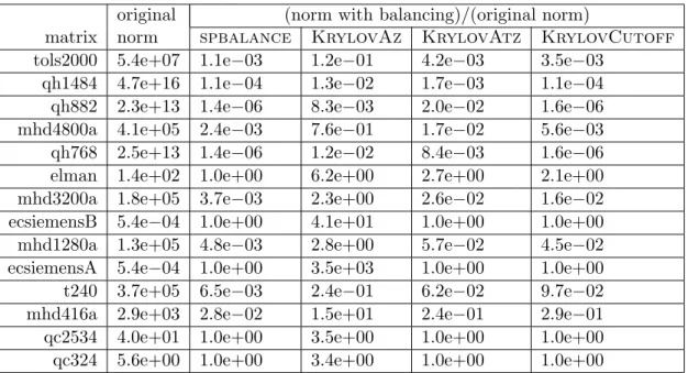
Krylov-based balancing algorithms do, in fact, often improve the accuracy to which eigenvalues are computed by dense or sparse eigensolvers. For our test matrices, Krylov-based balancing improved the accuracy of eigenvalues computed by sparse eigensolvers by up to 10 decimal places. In addition, Krylov-based balancing can also improve the condition number of eigenvalues, hence giving better computed error bounds.

For solving sparse systems of linear systems the problem is to find a vectorx such thatAx=b, whereAis a square nonsingular matrix andbis some given vector. Algorithms for findingxcan be classified as either direct or iterative: direct methods typically compute the LU factorization of A and solve forx through two triangular solves; iterative methods such as conjugate gradient iteratively improve on an initial guess to x. Though direct methods are considered robust, they can require large amounts of memory if the L and U

factors have many more nonzero elements than the matrixA. On the other hand, though iterative methods require less space, they are also less robust than direct methods and their behavior is not as well understood.

Fortunately, preconditioning can help with some of these issues. For example, preconditioners can be used to reduce the number of nonzero elements in the L and U

factors ofA, or to improve the likelihood of an iterative method converging quickly to the actual solution vector.

We begin by discussing preconditioners for direct solvers, starting with several algorithms for reordering the rows and columns ofA prior to factoring it. We present data comparing the results of decomposing matrices with a nonsymmetric permutation to results from using a symmetric permutation. For one matrix the size of the largest block found with a nonsymmetric permutation is a tenth of the size of the largest block found with a symmetric permutation, which can greatly reduce the subsequent factorization time. We also note that using a stability ordering in concert with a column approximate minimum

(6)

degree ordering can lead toLandU factors with significantly more or fewer nonzero elements than those computed after using the sparsity ordering alone.

Focussing on a specific algorithm for reordering A to reduce fill, we then describe our design and implementation of a threaded column approximate minimum degree algo-rithm. Though we worked hard to avoid the effects of many known parallel pitfalls, our final implementation never achieved a speedup of more than 3 on 8 processors of an SGI Power Challenge machine, and more typically there was virtually no speedup. By analyzing the performance of our code in detail, we provide a better understanding of the difficulties of efficiently implementing algorithms with fine-grained parallelism even in a shared memory environment.

Finally we turn to incomplete LU (ILU) factorizations, a family of preconditioners often used with iterative solvers. We propose a modification to a standard ILU scheme and show that it makes better use of the memory the user has available, leading to a greater likelihood of convergence for preconditioned GMRES(50), the iterative solver used in our studies. By looking at data gathered from tens of thousands of test runs combining matrices with different ILU algorithms, parameter settings, scaling algorithms, and ordering algorithms, we draw some conclusions about the effects of different ordering algorithm on the convergence of ILU-preconditioned GMRES(50). We find, for example, that both ordering for stability and partial pivoting are necessary for achieving the best convergence results.

Professor James W. Demmel Dissertation Committee Chair

(7)

List of Figures

1.1 Example of a matrix stored in column compressed format . . . 3

2.1 Example of Parlett-Reinsch decomposition . . . 15

2.2 Example of strongly connected components decomposition . . . 16

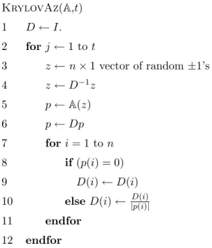
2.3 Pseudocode for the iterative balancing algorithm. . . 24

2.4 Pseudocode forKrylovAz. . . 28

2.5 Pseudocode forKrylovAzifAnot given explicitly. . . 29

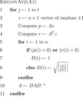
2.6 Pseudocode forKrylovAtz. . . 30

2.7 Accuracy of the eigenvalues of qh768 computed with and without direct bal-ancing. . . 34

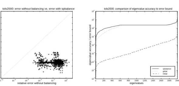
2.8 Accuracy of the eigenvalues of tols2000 computed with and without direct balancing. . . 35

2.9 Accuracy of the eigenvalues of qh768 computed with and without Krylov-based balancing. . . 36

2.10 Accuracy of the eigenvalues of tols2000 computed with and without Krylov-based balancing. . . 36

2.11 Relative accuracy of the largest and smallest eigenvalues of qh768 computed with Krylov-based balancing. . . 38

2.12 Relative accuracy of the largest and smallest eigenvalues of tol2000 computed with Krylov-based balancing. . . 38

3.1 Pseudocode for parallel approximate minimum degree algorithm. . . 55

3.2 Pseudocode for ILUTP. . . 89

3.3 Number of nonzeros in each row of the incomplete factors of shyy41 and vavasis1. . . 91

3.4 Pseudocode for ILUTP Push. . . 92

(10)

List of Tables

2.1 Effects of different symmetric decomposition algorithms . . . 17

2.2 Summary of known results on matrix norm minimization via diagonal scaling 23 2.3 Summary of known results on balancing matrices . . . 24

2.4 Effect of Krylov balancing algorithms on matrix norms . . . 31

3.1 Decompositions with scc vs. dmperm. Part 1. . . 46

3.2 Decompositions with scc vs. dmperm. Part 2. . . 47

3.3 Number of iterations taken by threaded column approximate minimum de-gree code with different parameter settings. . . 60

3.4 Breakdown of time taken by threaded column approximate minimum degree algorithm. . . 65

3.5 nnz(L+U) for different orderings. Part I. . . 70

3.6 nnz(L+U) for different orderings. Part II. . . 71

3.7 Summary of packages including IC or ILU algorithms. . . 82

3.8 Number of systems that converge with ILUTP and varied amounts of fill. . 88

3.9 Number of systems that converge with ILUTP and space used by factors. . 90

3.10 Number of systems that converge with ILUTP vs. ILUTP Push. . . 94

3.11 Number of matrices that converge with ILUTP vs. ILUTP Push with high fill and various pivtol . . . 95

3.12 Number of systems converging with ILUTP Push and space used by factors. 95 3.13 Number of systems that converge with different orderings for various levels of ILU(k). . . 100

3.14 Number of systems that converge with different orderings and ILUTP Push with varied amounts of fill. . . 101

3.15 Number of systems that converge with ILU(k) and ILUTP Push withnnz( ˆL+ ˆ U) =nnz(A). . . 102

3.16 Effects ofpivtolon convergence of ILUTP Push with different sparsity order-ings. . . 102

3.17 Number of systems that converge with ILU(k) with MC64 and different spar-sity orderings. . . 104

3.18 Number of systems that converge with ILUTP Push and MC64, but with different sparsity orderings. . . 104

(11)

3.19 Comparing ILU(k) and ILUTP Push with MC64 and fixed parameter values, but different sparsity orderings. . . 105 3.20 Effects of differentpivtolvalues and sparsity orderings on ILUTP Push with

MC64. . . 106 3.21 Number of systems converging with ILU(k), MC64 with scaling, and different

sparsity orderings. . . 107 3.22 Number of systems converging with ILUTP Push, MC64 with scaling, and

different sparsity orderings. . . 107 3.23 Difference between ILU(k) and ILUTP Push with MC64 and scaling, but

different sparsity orderings. . . 108 3.24 Effects ofpivtolon convergence of ILUTP Push with MC64 and scaling, but

(12)

Acknowledgements

For helping with research, I should first thank my advisor Jim Demmel, my com-mittee members Jonathan Shewchuck and Greg Fenves, and my qualifying examination chair Kathy Yelick. I would also like to thank Sivan Toledo and John Gilbert for having me spend a summer at Xerox PARC; and Esmond Ng for having me spend two summers at NERSC. Other people I have had useful discussions with include: Beresford Parlett (on balancing), David Hysom (on ILU preconditioners), Brent Chun and Fred Wong (on the innards of the Berkeley NOW and Millennium), and Henry Cohn (on a variety of math topics).

Of course, I also need to thank the agencies whose grants funded me. This research was supported in part by an NSF graduate fellowship and in part by LLNL Memorandum Agreement No. B504962 under the Department of Energy under DOE Contract No. W-7405-ENG-48, and the National Science Foundation under NSF Cooperative Agreement No. ACI-9619020, and DOE subcontract to Argonne, no. 951322401. The information presented here does not necessarily reflect the position or the policy of the Government and no official endorsement should be inferred.

Some of my richest experiences at Berkeley had nothing to do with research. Linh, Thanh Thao, Herman, Rahel and Leya, Peter, Tsedenia, Kedest, Salma, Saana, Fatima, and many others: thank you for giving me a clearer sense of myself and a more complete picture of our world.

(13)

Chapter 1

Introduction

As processor speeds and storage capacities increase, people expect computers both to solve existing problems more quickly and to solve larger and more complex problems. In the field of linear algebra, the latter corresponds to solving systems with large, potentially ill-conditioned matrices. The storage requirements for large matrices can sometimes be reduced if they aresparse, ie. if many of the matrix entries are zero. Furthermore, the time and memory needed to solve a large system can sometimes be reduced bypreconditioning the system prior to solving it.

Informally, to precondition a system prior to computing a solution is to transform it into one with more desirable properties. The solution to the altered system is computed, and transformed into the solution of the original problem. The advantages of solving the modified system can include more accurate results, decreased running time, reduced memory requirements, or some combination of these. What makes a preconditioner desirable can depend on both the problem and the solution method.

In this dissertation we look at preconditioners for two classes of linear algebra problems: eigenproblems and linear systems. In chapter 2 we discuss preconditioning for sparse eigenproblems, considering both how to permute a matrix to decompose it, and how to balance a matrix to improve the accuracy of its computed eigenvalues. In chapter 3 we turn to preconditioning for linear systems. We discuss heuristics for permuting the rows and columns to achieve goals such as decomposing the matrix, reducing the number of nonzeros in the factors, and stabilizing the matrix. We then look at incomplete LU factorizations, a class of preconditioners for iterative solvers.

(14)

of storage and algorithmic issues concerning sparse matrices, and of the roles of precondi-tioners for direct and iterative solvers. We then define some of the matrix notation and graph representations used throughout this report, and end with a summary of our contri-butions.

1.1 Sparse systems

As noted, we are interested primarily in sparse matrices, which can be thought of asnby m matrices with enough zero elements to make storing only the nonzero elements, and not all nmentries, worthwhile. Sparse algorithms which ignore the zero elements can sometimes be faster than their dense counterparts which operate on all entries. For example, consider an n by n diagonal matrix. Clearly storing only the n nonzero diagonal entries is cheaper than storing all n2 _{matrix elements. Clearly algorithms which ignore the zero}

off-diagonal elements can be far more efficient than those which do not. For example, if computing the diagonal matrix times a vector, the standard dense algorithm computes n

dot products of lengthn, whereas a sparse algorithm operating only on the nonzero elements requires nscalar multiplications.

In practice, sparse matrices arise in many application areas. For example, when simulating the effects of applying heat to a plate or the flow of air around an airplane wing, the first step is often to model the plate or the wing by putting a mesh on it. This mesh can be seen as an undirected graph withv vertices andeedges. If we translate this graph into a matrix, a process better described in section 1.3.2, the matrix is av×v matrix with 2e nonzeros. Since two vertices are connected by an edge only if they are near each other in the physical object, the number of edges is much smaller than v2_/_{2. If we model a 2D}

square plate by putting ann×nmesh on it, the matrix will havev=n2 _{rows and columns,}

and only 5n2₋₄_n_{, rather than}_n4 _{nonzero entries.}

As the matrix-vector multiplication example shows, we need both data structures for storing sparse matrices and algorithms that take advantage of the sparse storage formats. Because sparse matrices are less structured than dense matrices, creating either of the two can be challenging.

(15)

1.1.1 Storage of sparse matrices

Traditionally dense matrices have been stored as a two-dimensional array in ei-ther column-major or row-major order, though more recent work suggests performance advantages to using recursive layouts [4, 67, 94]. For sparse matrices, on the other hand, significantly more storage methods are used. The range of possibilities comes from the fact that matrices from different applications have different nonzero structures (eg, that the diagonal of the matrix may be nonzero, or that the matrix has a narrow band), and that different matrix representations allow for efficient implementation of different operations.

Column-compressed format is a very popular sparse matrix representation that some large matrix repositories, including the Harwell-Boeing collection [55] and the Uni-versity of Florida sparse matrix collection [47], use. As the small example in figure 1.1 shows, the column-compressed format stores a sparse matrix with real entries in three ar-rays: nzval, rowind, and colptr. The nzval array hasnnzelements, wherennzis the number of nonzeros in the matrix. The elements in nzval are the values of the nonzero elements, stored by column, so that the elements in column 1 are listed first, then those in column 2, and so on. The integer array rowind also hasnnz entries and rowind[i] is the row index of the entry whose value is stored in nzval[i]. The integer array colptr has n+ 1 entries, where nis the number of columns in the matrix, and colptr[i] is the location in nzval and rowind where the first element in columnican be found. Equivalently, colptr[i] is the total number of nonzeros in columns 1 throughi−1. The first entry, colptr[0], has value 0, and the last entry, colptr[n+ 1], has value nnz. Although in the example the elements in each column are sorted by increasing row index, this is not a requirement of the format.

2 1 2 3 4 5 6 7 8 1 3 4 5 6 7 8 0 2 1 2 3 0 3 2 0 2 5 7 8 nzval colptr rowind

Figure 1.1: This figure shows how a small sparse matrix is stored the compressed column format (also know as the Harwell-Boeing format).

(16)

sys-tems described in section 3.4, is the row-based analogue of column-compressed format: matrix entries are stored by row instead of by column. The row-compressed format uses rowptr and colind arrays in place of the colptr and rowind arrays.

We describe less common storage formats as necessary throughout the report. Books such as [14] and [148] describe some of the many other sparse matrix storage represen-tations people use. In principle, one could devise arbitrary hybrids of these to accommodate particular applications, as done in [107, 109, 175].

1.1.2 Sparse matrix algorithms

Just as we have an understanding of good storage methods for dense matrices, we also know how to exploit the memory hierarchy to write efficient dense linear algebra code. The goal is to limit the amount of data movement between levels of the memory hierarchy. The trick is toblock the matrix, which divides it into smaller non-overlapping submatrices, and then to operate on the individual blocks. The operations on these smaller blocks should all fit into the lowest level (the one with the most storage) of the memory hierarchy. Since there are typically several levels in the memory hierarchy, the submatrices themselves may be again divided into smaller subblocks which are also operated on one at a time. Typically the memory needed to store the largest blocks is on the order of the size of the first level cache and the number of elements in the smallest blocks is on the order of the number of floating point registers.

Blocking can be very effective for dense matrix computations because they typically access matrix and vector elements in regular patterns. Unfortunately, sparse matrices are not as structured as dense matrices and in general cannot be easily blocked into small dense subblocks. Memory references tend to be irregular, which makes exploiting temporal or spatial locality difficult. Of course, if a user knows his or her application generates sparse matrices with small dense subblocks, performance can be improved by using algorithms that can exploit this feature. Other work looks at padding sparse matrices by storing some zero elements in order to create dense blocks [107, 108, 109, 175]. Nevertheless, overall, achieving high performance on sparse matrix computations remains a complex open problem.

Although algorithms operating on matrices stored in sparse matrix representa-tions can be difficult to code efficiently, some algorithms may be easier to implement on sparse matrices. For example, graph algorithms translate nicely to sparse matrices stored

(17)

in row compressed format, which is essentially the same as the standard adjacency graph representation of a matrix.

1.2 Roles of preconditioning

As noted, preconditioning a system alters it so that the changed system is somehow “better”. The answer to the improved system is computed, and from it the answer to the original system is derived. What makes the preconditioned system “better” depends largely on how the algorithm then used to solve the preconditioned system works.

For example, consider direct versus iterative methods, a categorization we use to describe algorithms throughout this report. Informally, a direct method is an algorithm that is usually run for a fixed number of steps, at the end of which it almost always returns an answer that is sufficiently close to the exact solution that it is often considered exact, modulo roundoff error. An iterative method, on the other hand, begins with an initial guess to the solution and iteratively tries to improve it. The algorithm stops either when the approximation is deemed sufficiently close to the exact solution, or when some large number of iterations has been run and the user suspects the algorithm has stagnated and so a good approximate solution may never be reached. We note that some methods (for example, the conjugate gradient solver for linear systems [100]) span direct and iterative methods in the sense that they compute the exact answer innsteps in exact arithmetic, but in practice are used as iterative methods either because they often compute a reasonable solution in far fewer thannsteps or because the iterations are expensive and nis large.

The motive for preconditioning differs for iterative and direct methods. Since a direct method gives the answer after running for a fixed number of steps, a useful precon-ditioner might turn the system into one where each step takes less time, or one for which the solver computes a more accurate answer. For an iterative method, on the other hand, an effective preconditioner might create a system for which the iterative solver converges when it did not for the original problem, a system where the number of iterations needed for convergence is reduced, or one where each iteration can be computed more efficiently.

However, accuracy of the solution and the speed with which that solution is com-puted remain paramount. Because of the latter, preconditioners are judged not only by how much they improve the performance of the solver, but also by other measures such as the cost of computing and applying that preconditioner. Since the preconditioner must be

(18)

first computed prior to solving the modified system, it should be relatively inexpensive to compute. Note that if many similar systems are to be solved and the same preconditioner is used for all of them, the cost of computing the preconditioner can potentially be amortized. After solving the preconditioned system the effects of the preconditioner must be undone to recover the solution to the original problem; this step should also be inexpensive. Further-more if the preconditioner will be applied in every iteration of the algorithm, as with the incomplete LU preconditioner discussed in section 3.4, the application of the preconditioner should be inexpensive.

The tradeoff between the time needed to compute and apply the preconditioner, and the time saved and accuracy gained with a high quality preconditioner is an issue throughout this report.

1.3 Notation and Definitions

The discussions in this report move between matrix and graph terminology. To smooth the transitions between the two, in this section we summarize our matrix notation, define the graphs associated with a matrix, and discuss relationships between matrix and graph terminology.

1.3.1 Matrix notation and definitions

We generally use capital letters for representing matrices, lower case letters for vectors, and Greek letters for constants. A few letters are reserved for special matrices: A, which refers to the n×n, possibly nonsymmetric, matrix being preconditioned; B, which is A after preconditioning; P and Q, which are permutation matrices; and D, which is a diagonal matrix. The vectoreis the vector whose entries are all 1. The number of nonzero elements in a matrix M is denoted bynnz(M).

In the context of solving a system of linear equations, we use Land U to denote the complete LU factors ofA, soA=LU if no pivoting is used. With row pivoting, we have

P A=LU; with column pivoting we haveAP =LU. We use ˆLand ˆU to denote incomplete factors of A, so ˆLUˆ ≈ A. The number of nonzeros in the incomplete factorization is nnz( ˆL+ ˆU), and we will typically denote the number of nonzeros in a matrixAbynnz(A), though the (A) may be omitted if the context clearly specifies the matrix.

(19)

We frequently use Matlab notation when referring to elements in vectors and matrices. For example, we use colons to indicate a sequence of indices, soA(i,:) is row iof

A, and A(3 : 5,:) is the submatrix consisting of the third, fourth, and fifth rows of A. For more information on Matlab notation, see [133].

If a permutation P is applied symmetrically, it mapsAtoP APT_.

If A is anonnegativematrix, it has no negative entries. This may also be written as A≥0. If A is real and symmetric,A =AT_{. If} _A _{is complex and} _Hermitian,_A ₌_AH_.

If A isstructurally symmetric,A and AT _{have nonzeros in the same locations, though the}

values may differ. Finally, |A|is shorthand for the matrix whose entries are|A(i, j)|. We usenormsto measure the “size” of vectors and matrices, where the norm ofx

is written as kxk. Ifxis a lengthn vector, some of the vector norms we use are defined as follows:

1−norm: kxk1 ≡ |x1|+|x2|+. . .+|xn|

2−norm: kxk2 ≡ (|x1|2+|x2|2+. . .+|xn|2)1/2

∞ −norm: kxk∞ ≡ maxi{|xi|}

IfA is ann×nmatrix, some of the matrix norms we use are defined as follows:

1−norm: kAk₁ ≡ max_j{P_i(A(i, j))}

2−norm: kAk2 ≡ max{λ1/2 :λis an eigenvalue ofAHA}

∞ −norm: kAk∞ ≡ maxi{

P

j(A(i, j))}

Froebenius norm: kAk_F ≡ ³P_i,j{|A(i, j)|2_}´1/2

For more on norms, look in linear algebra books such as [52, 82, 102].

The condition number of a matrix A with respect to a particular problem is a measure of how sensitive the solution to that problem is to perturbations inA. The condition number of A with respect to matrix inversion is defined as κ(A) = kAkkA−1_k _if _A _is

nonsingular and κ(A) =∞ ifA is singular. Again, for more information consult books on linear algebra such as [52, 82, 102].

Other less frequently used terms will be defined when they are first used. 1.3.2 Graph representations of matrices

We now describe two ways of representing matrices by a graph, both of which are often referred to in the literature. There are the directed graph and the bipartite graph

(20)

representations; given a matrix A we refer to the first graph as DG(A), and the latter as

BG(A). Note the latter is sometimes called the dependency graph ofA(e.g., in [131]). When discussing graphs we use common graph terminology. For example, let a graph G be defined by a set of vertices V and a set of directed edges from one vertex to anotherE. Then, apathfrom vertexstotis a list of vertices (s, v1, v2, . . . , vk, t) such that

there are directed edges in E from s to v1, from vi to vi+1 for all 1 ≤ i < k, and from

vk to t. We also refer later on to the subgraph induced by a set of vertices, and mention

graph algorithms such as depth first search. The terminology and algorithms can be found in standard algorithm textbooks such as [1, 44].

Directed graph representation

Annbynunsymmetric matrixAcan be represented by a directed graphDG(A) = (V, E), where |V|=n, and the directed edge (i, j)∈E if and only ifA(i, j)6= 0.

If we need a weighted graph DG_w(A), the weight on edge (i, j) is the value of

A(i, j). If A is an n by m matrix where n6=m, then |V|= max(n, m) and either some of the nodes will have no incoming edges or some will have no outgoing edges, depending on whether A has more rows or more columns. Thus DG(A) is the same asDG( ¯A) where ¯A

is gotten by extendingA with enough zero rows or columns to make it square. Bipartite graph representation

Alternatively, annby nunsymmetric matrixAcan be represented by a bipartite graph BG(A) = (R, C, E). In this representation |R|=|C| =n, and the undirected edge (ri, cj) exists if and only ifA(i, j)6= 0.

If a weighted graph BG_w(A) is needed, the weight on the edge (r_i, c_j) is the value of A(i, j). IfA is not square, the only change is that |R| 6=|C|.

1.3.3 Relationships between A, DG(A), and BG(A)

We now point out some obvious, and some perhaps not so obvious, relationships between a matrix and its associated graphs. For example, note that entries on the diagonal of Acorrespond to self-edges inDG(A).

Now consider the case where A is a structurally symmetric matrix. This means

(21)

edge (i, j) in DG(A) implies the existence of the edge (j, i). Of course, if we need edge weights, Aneeds to be symmetric, not just structurally symmetric, forDG(A) to be repre-sentable by an undirected graph. InBG(A) = (R, C, E), symmetry inA is reflected in the fact that if edge (r_i, c_j)∈E, then (r_j, c_i)∈E.

Although the nodes in a graph are typically not thought of as ordered in any way, the rows and columns of a matrix are always ordered (i.e., we refer to the first row or third column of a matrix). If we think of the nodes in DG(A) as numbered so that the node corresponding to the first row and column of A is node 1, a reordering of the nodes corresponds to permuting the rows and columns of A symmetrically (i.e., P APT). This makes DG(A) useful for algorithms that permute the rows and columns of a matrix symmetrically, such as some of those described in section 3.2.1. Renumbering the nodes of DG(A) is no longer appropriate if different permutations are applied to the rows and columns ofA (i.e.,P AQT_{), so the bipartite representation}_BG₍_A_{), which allows the nodes}

of R andC to be numbered separately, is often used instead in this situation.

Finally, recall that a square matrix A is irreducible if there is no permutation matrixP such that

A=   X Y 0 Z  

whereX andZ are square. If such aP does exist,Aisreducible. IfAis irreducible,DG(A) is strongly connected, which means there is a directed path from any vertex to any other (e.g., [52, lemma 6.6]).

1.4 Test Matrices

The algorithms we describe in this report are tested on assorted matrices from a variety of applications. Because the performance of an algorithm depends on the matrices it is tested on, in this section we describe how we chose our test matrices.

First we chose matrices from a range of application areas. By not biasing our matrices towards any one domain, we hoped our algorithms would be similarly unbiased and would work well for more than very specific types of matrices. Of course, if a user knows his or her matrices all share some common structure, the best algorithms for them will likely take advantage of that structure. Furthermore we chose matrices that spanned a range of sizes and densities.

(22)

The matrices used in chapter 2 are taken from a collection of non-Hermitian eigen-value problems [10]. These matrices are all specifically from eigenproblems. As the table in appendix A shows, the matrices used are of modest size and come from a range of applications.

The matrices used in chapter 3 come from a variety of collections, with the majority of them available from either the Matrix Market [15] or the University of Florida sparse matrix collection [47]. Previous work on direct and iterative solvers also analyzes results of experiments conducted on a variety of matrices so to make comparisons between our results and those from previous work, we tried to ensure some overlap between our test suite and those from assorted other papers. Furthermore, since the size of sparse linear systems that computers can handle continually increases, we also tried to add new, larger matrices. The table in appendix B provides more details about the matrices chosen.

1.5 Contributions

The contributions of this work are as follows. In chapter 2 we consider the problem of computing the eigenvalues of a sparse matrix, that is findingλ such thatAx=λx. We first notice that decomposing the matrix A into irreducible components can significantly reduce the expected time complexity of finding the eigenvalues of A. This scheme can be arbitrarily better than the conventional scheme used for dense matrices, described in [147] and used in packages such as Lapack [5] and Eispack [169].

We then define the concept of balancing in a weighted norm, show how to balance non-negative, irreducible matrices in the weighted norm, and prove this balancing minimizes the 2-norm of such matrices. The idea of a balancing in a weighted norm is used to justify a novel set of Krylov-based algorithms which balance a matrix without accessing its indi-vidual entries. By using only matrix-vector (Ax), and sometimes matrix-transpose-vector (AT_x_{), multiplications to access}_A_{, these new algorithms can be used with eigensolvers that}

similarly assume only that a subroutine for computingAx(and possiblyAT_x_{) is available.}

Finally we show that for matrices from our test suite Krylov-based balancing algorithms can improve the accuracy to which eigenvalues are computed by as much as 10 decimal places for sparse eigensolvers. Furthermore, Krylov-based balancing can also improve the condition number of the eigenvalues, which improves computed error bounds.

(23)

find x such that Ax = b. Direct solvers first factor the matrix A, so we begin by dis-cussing various reasons for reordering the rows and columns ofA prior to factoring it. We present data showing the advantages of decomposing the matrices in our test suite through a nonsymmetric permutation rather than the symmetric strongly connected components decomposition used when computing eigenvalues. For one matrix in our test suite the size of the largest block found with a nonsymmetric permutation is a tenth of the size of that found with a symmetric permutation, which can greatly reduce the subsequent factorization time. We also note in section 3.3.2 that using a stability ordering in concert with a column approximate minimum degree ordering can lead to fill in the LU factors that differs signif-icantly from that of using the sparsity ordering alone. On our test matrices the difference between the two could be up to a factor of 2.

Focussing on one specific algorithm for reordering A, we next describe our design and implementation of a threaded column approximate minimum degree algorithm. Even after the extensive analysis and code modifications we describe, our final implementation never achieved a speedup of more than 3 on 8 processors of an SGI Power Challenge ma-chine, and more typically there was virtually no speedup. This work, done jointly with Sivan Toledo and John Gilbert [37], gives us a better understanding of the difficulties of efficiently implementing algorithms with fine-grained parallelism even in a shared memory environment.

Finally we turn to incomplete LU (ILU) factorizations, a family of preconditioners often used with iterative solvers. We propose a modification to a standard ILU scheme and show that it makes better use of the memory the user has available, leading to a greater likelihood of convergence for preconditioned GMRES(50), the iterative solver used in our studies. By looking at data gathered from tens of thousands of test runs combining matrices with different ILU algorithms, parameter settings, scaling algorithms, and ordering algorithms, we draw some conclusions about the effects of different ordering algorithm on the convergence of ILU-preconditioned GMRES(50). We find, for example, that both ordering for stability and partial pivoting are necessary for achieving the best convergence results.

(24)

Chapter 2

Preconditioning sparse matrices for

computing eigenvalues

Given a matrixA, we say thatλis an eigenvalue ofAwith corresponding eigenvec-torx ifAx=λx andx6= 0. Given A, eigensolvers try to find some or all of its eigenvalues and eigenvectors. The eigenvalues of a matrix are maintained under similarity transforms, which means the eigenvalues ofB =SAS−1, whereS is nonsingular, are the same as those of A. The eigenvectors, on the other hand, are transformed by S so if x is an eigenvector of A,Sx is an eigenvector of B. Preconditioning in this context means choosingS so that the eigenvalues of SAS−1 _{can be computed more quickly or more accurately than those of}

the untransformedA.

In this chapter we explore two methods for choosingS. In section 2.1 we constrain

Sto be a permutation matrix and show how to decomposeAinto a set of smaller systems. In section 2.2 we then constrainS to be a diagonal matrix and look at algorithms for scaling the entries of A to improve the accuracy with which its eigenvalues can be computed. These techniques can sometimes be combined, and in section 2.3 we show the effects of preconditioning on the accuracy of computed eigenvalues.

Our contributions are first to notice that decomposing a matrix A by using a strongly connected components algorithm can significantly reduce the expected time com-plexity of finding the eigenvalues of A. This scheme can be arbitrarily better than the conventional scheme used for dense matrices, described in [147] and used in packages such as Lapack [5] and Eispack [169].

(25)

We then switch gears and define weighted balancing, which we show minimizes the 2-norm of a nonnegative matrix. We further describe novel Krylov-based balancing algo-rithms which approximate weighted balancing and which operate on a matrixAwithout ex-plicitly accessing its entries. By using only matrix-vector, and sometimes matrix-transpose-vector, multiplications to accessA, these new algorithms can be used with eigensolvers that similarly assume only that a subroutine for computingAx(and possiblyAT_x_{) is available.}

Finally we show that for matrices from our test suite, these Krylov-based balancing algorithms do, in fact, often improve the accuracy to which eigenvalues are computed by dense or sparse eigensolvers by as much as 5 decimal places in our examples with dense eigensolvers and as much as 10 decimal places for sparse eigensolvers. Furthermore, Krylov-based balancing can also improve the condition number of the eigenvalues, which improves computed error bounds.

Portions of this work were published in [33, 35, 36].

2.1 Decomposing the matrix

We first consider choosing a similarity transform P, where P is a permutation matrix. The goal is to findP such that:

P APT =   X Y 0 Z  _,

where X and Z are square. Since the eigenvalues of A are the eigenvalues of X together with those of Z, this decomposition reduces the problem of finding the eigenvalues of Ato the smaller, and therefore simpler, eigenproblems for X and Z. Recall from section 1.3.3 that if such aP exists, A is reducible, otherwiseAis irreducible.

P is applied symmetrically, so the transformation permutes the rows and columns ofAin the same way. Looking at DG(A) andDG(P APT_{) (defined in section 1.3.2) we see}

the two are isomorphic, and only the numbering of the nodes is changed.

In this section we review an algorithm for finding P described by Parlett and Reinsch in [147] and used by codes in several popular linear algebra libraries. We then describe a permutation which can do significantly better and end with a comparison of the two algorithms on our test matrices.

(26)

2.1.1 The Parlett-Reinsch Algorithm

In [147] Parlett and Reinsch describe a two-step algorithm for transforming a matrix prior to computing its eigenvalues. In the first step, the matrix is permuted to separate out rows and columns which isolate eigenvalues. In the second, the remaining rows and columns are scaled. This algorithm is implemented in linear algebra packages such as EISPACK (under the name balanc), LAPACK (under the name gebal1), and

MATLAB(under the name balance).

In the permutation phase, the algorithm first searches for a row with zeros on all

n−1 off-diagonal entries. If a row with this structure exists, it is permuted to the bottom of the matrix by swapping two rows and swapping the same two columns. The algorithm then iterates on the first n−1 rows and columns of the permuted matrix. When no more rows isolating eigenvalues on the diagonal are found, the process repeats for columns. Afterwards the algorithm has found a permutation matrixP such that

PTAP =     T1 X Y 0 C Z 0 0 T2     (2.1)

where T₁ and T₂ are upper triangular. The eigenvalues of T₁ and T₂ are their diagonal entries. Even though the square submatrixC may not be irreducible, this decomposition is deemed sufficiently good.

In graph theoretic terms, this algorithm begins by looking for a sink node s of

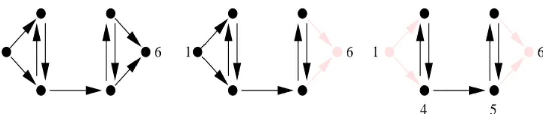
DG(A). If one exists, it is given the number n, meaning in the permuted matrix it cor-responds to the last row and column. The algorithm then looks for a sink node in the subgraph induced by the set of all nodes excepts. If a sink node exists in this subgraph, it is numberedn−1. When there are no sink nodes found in the last subgraph the algorithm then continues by looking for source nodes, which are numbered in increasing order, starting with 1. Nodes not identified as source or sink nodes end up numbered after all the source nodes and before all the sink nodes. See figure 2.1 for a small example.

1_In_LAPACK_{there is also an additional character at the beginning of the subroutine name which specifies}

(27)

6 1 6 1 6 3 2

4 5

(a) (b) (c)

Figure 2.1: This figure shows how the Parlett-Reinsch algorithm would decompose a small graph. In (a) a sink node is located and numbered last; in (b) there are no sink nodes, so a source node is located and numbered 1; in (c) there are neither sink nor source nodes so the remaining nodes are considered a group and numbered consecutively. Gray elements were eliminated in a previous step and are not considered.

2.1.2 The Strongly Connected Components Algorithm

By locating individual rows and columns which isolate eigenvalues, the permu-tation phase of the Parlett-Reinsch algorithm finds a permupermu-tation matrix P which makes

P APT _{as upper triangular as possible. In other words, it decomposes}_A_{into 1}_×_{1 blocks and}

one large block consisting of all the remaining rows and columns, as shown in equation 2.1. We suggest choosingP to makeP APT _{as block upper triangular as possible, which}

decom-posesAinto a set of diagonal blocks of size ˆn₁,nˆ₂, . . . ,nˆ_k, wherekdepends on the structure of the matrix. This minimizes the size of the largest diagonal block which is significant since that a dense eigensolver on the decomposed matrix runs in timeO(Pk_i₌₁ˆn3

i).

In graph theoretic terms, making A as block upper triangular as possible corre-sponds to finding the strongly connected components of a directed graph whose adjacency matrix has the same structure as A and then sorting the components using a topological sort [44, section 23.5]. See figure 2.2 for a small example.

Tarjan noted that finding the strongly connected components of a directed graph can be done using two depth first searches [173]; a description of his algorithm can be found in [1, section 5.5]. Descriptions of implementations are in [59] and [151]. We point out that Tarjan’s algorithm is particularly well suited to this application because it outputs the nodes one strongly connected component at a time, with the components already topologically sorted.

PermutingA to block upper triangular form means the indices of several diagonal blocks may need to be stored so that the eigenproblems corresponding to these blocks

(28)

1 2 3 4 5 6

Figure 2.2: This figure shows how the strongly connected components algorithm would decompose a small graph. All the strongly connected components are located, then a topo-logical sort is done on the components, and the nodes are numbered so that if componenti

comes after component jin the topological sort, all elements of componentihave numbers greater than those of the elements of component j.

can be identified and solved. However, we believe the potential benefits of this algorithm over the Parlett-Reinsch algorithm compensate for the additional complexity. Because the eigenvalues of the original matrix A are the same as the union of the eigenvalues of the individual diagonal blocks inPT_AP_{, the running time of any eigensolver run on the blocks}

of the balanced matrix depends strongly on the size of the largest block. The size of the largest diagonal block found using this permutation can be significantly smaller than that found by the Parlett-Reinsch algorithm, and it is never larger.

2.1.3 Comparisons

The benefits of using the strongly connected components algorithm instead of the Parlett-Reinsch algorithm are two-fold. First, as described in the next paragraph, computing the strongly connected components is likely to take less time for sparse matrices stored in compressed format (row or column). Second, the size of the largest diagonal block can be much smaller with the strongly connected components algorithm, which makes computing the eigenvalues ofA less expensive.

The Parlett-Reinsch permutation algorithm permutes rows one at a time, which requires O(nnz) time for each row if the matrix is in compressed column format. For a permuted upper triangular matrix, the permutation phase would takeO(nnz·n) time, which is much more than theO(n+nnz) time taken by Tarjan’s strongly connected components algorithm. In short, it is more efficient to run an algorithm that needs only two sweeps through the entire data structure to identify all the blocks, rather than one which repeatedly looks for a single 1 by 1 block in each sweep.

(29)

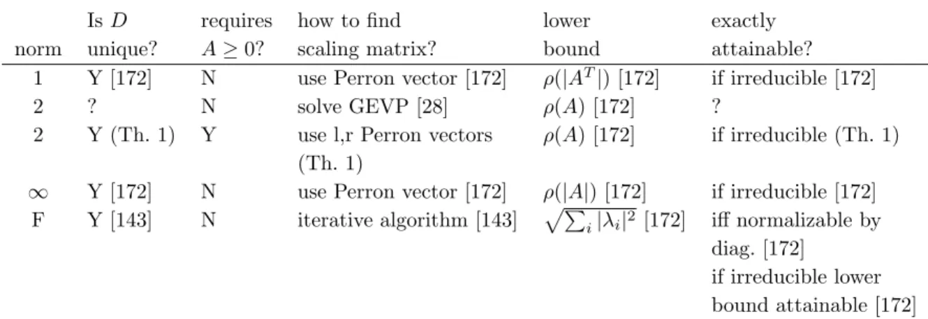
strongly conn. comp. Parlett-Reinsch name n # scc max(blocks) P(blocks3) max(blocks) P(blocks3)

tols2000 2000 1529 90 7.33e5 854 6.23e8

t240 240 121 90 7.29e5 150 3.38e6

ecsiemensA 177 6 167 4.66e6 177 5.54e6

ecsiemensB 177 26 151 3.44e6 153 3.58e6

qh1484 1484 3 1470 3.18e9 1484 3.27e9

qh882 882 1 882 6.86e8 882 6.86e8

mhd4800a 4800 8 4793 1.10e11 4793 1.10e11

qh768 768 1 768 4.53e8 768 4.53e8

mvmpde 900 1 900 7.29e8 900 7.29e8

mhd3200a 3200 8 3193 3.26e10 3193 3.26e10

mhd1280a 1280 15 1266 2.03e9 1266 2.03e9

mhd416a 416 8 409 6.84e7 409 6.84e7

qc2534 2534 1 2534 1.63e10 2534 1.63e10

qc324 324 1 324 3.40e7 324 3.40e7

Table 2.1: This table shows the number of strongly connected components (# scc) found in matrices in the test suite as well as the size of the largest component (max(block)). The size of the submatrix C, as defined in Equation 2.1, from the Parlett-Reinsch algorithm is given for comparison. As a measure of how long an O(n3_{) algorithm would take to}

find the eigenvalues of the decomposed matrix, we give the sum of the block sizes cubed (P(blocks3)). The matrices are sorted so that the matrices helped most by finding strongly connected components are listed first: the largest block is reduced significantly for tols2000 and t240, reduced somewhat for ecsiemensA, ecsiemensB, and qh1484, and reduced not at all for the other matrices.

Furthermore, the largest block found via strongly connected components can be much smaller than that found by the Parlett-Reinsch algorithm. Table 2.1 shows the number of strongly connected components found for each of the test matrices, together with the size of the largest block found by each permutation algorithm. As a measure of how long an

O(n3_{) algorithm would take to compute the eigenvalues of the decomposed matrices, we}

also give the sum of the diagonal block sizes cubed. Improvements, measured by this sum of cubes, range from 1 (no improvement) up to nearly 103_.

For information about these matrices, including the application areas from which they come, see appendix A.

(30)

2.2 Balancing

In the previous section we studied similarity transforms determined solely by the nonzero structure ofA. We now restrict ourselves to similarity transforms that are diagonal scaling matrices and hence depend on and affect the nonzero values inA.

Numerical algorithms that compute the eigenvalues of a nonsymmetric matrix A

typically have backward errors of the magnitude ofεkAk, whereεis the machine precision. Prior to computing the eigenvalues, applying a simple and accurate similarity transform

DAD−1_{, which reduces either the norm of} _A _{or the condition numbers of some subset of}

A’s eigenvalues, can be advantageous. For example, consider the matrix:

A=     1 0 10−4 1 1 10−2 104 ₁₀2 ₁    .

ChoosingD= diag(100,1, .01) gives:

B=DAD−1 =     1 0 1 10−2 _{1 1} 1 1 1    .

Whereas ||A||F, the Frobenius norm of A, is approximately 104, ||B||F is approximately

2.6. Furthermore, the condition numbers of the eigenvalues of B are all approximately 1, whereas those of the eigenvalues ofA range in magnitude from 101 _{to 10}3_{. Therefore, one}

expects to compute the eigenvalues of B more accurately than those of A. Notice B is balancedin the ∞-norm: a matrix is balanced in theα-norm if for anyi, theα-norm of row

iis the same as the α-norm of columni.

Osborne [143] showed balancing an irreducible matrix in the 2-norm is equivalent to minimizing its Frobenius norm; balancing a matrix in an arbitrary norm may not have such a simple effect on a matrix norm. Previous work studies the theory behind using diagonal scaling to balance matrices and to minimize matrix norms, as well as practical issues associated with implementing balancing algorithms. In this section we summarize and extend the theory of balancing before describing a family of balancing algorithms our theory suggests.

(31)

2.2.1 Theory

Before summarizing previous work on the theory of balancing and norm minimiza-tion, we note a few assumptions.

First, we consider primarily irreducible matrices. Recalling the relationship be-tween irreducible matrices and graphs as described in section 1.3.3, if a matrix is reducible, we can compute the strongly connected components of its graph using the algorithm de-scribed in section 2.1.2, and then consider the irreducible diagonal blocks individually. Furthermore, note that ifA is reducible with block structure [X Y; 0Z], the block Y can be scaled arbitrarily close to 0, without affecting the values inX and Z. In other words, if we partition the scaling matrix so D= [DX 0; 0DZ], the scaled matrix is:

DAD−1 =   DXXD−X1 DXY D−Z1 0 DZZD_Z−1  _. _(2.2)

IfD_Z is scaled by a large constant, the only change inDAD−1 _{is a decrease in the elements}

of D_XY D−_Z1. By increasing the constant, Y can be scaled arbitrary close to 0.

Furthermore, we typically do not consider the diagonal elements of the matrix. Not only are diagonal elements unaffected by balancing, but in most norms a matrix that is balanced when its diagonal elements are zero remains balanced when the diagonal elements are made non-zero. The converse is not true; if the diagonal entries are sufficiently large relative to the off-diagonal entries, the matrix will be nearly balanced regardless of the exact off-diagonal entries. Therefore balancing matrices with a zero diagonal is the more important case.

History

There are many interesting questions regarding the use of diagonal scale factors to balance a matrixAin some vector norm, or to minimize some matrix norm ofA. Questions pursued include whether exact balancing in a given norm is achievable, if the balancing matrix D is unique, and whether balancing in a given vector norm also minimizes some matrix norm ofA. In this section we summarize a few theoretical results from the literature on diagonal scaling. Tables 2.2 and 2.3 summarize the known results on balancing and norm minimization, and [33] contains a more complete overview.

Osborne [143] was the first to study balancing, showing that a matrix balanced in the 2-norm has minimal Frobenius norm. The iterative algorithm suggested by Osborne is

(32)

used in the Parlett-Reinsch algorithm [147], although the code provided in [147] balances in the 1-norm, which is cheaper to compute than the 2-norm.

For balancing in the 1-norm, Hartfiel [96] proved that ifAis irreducible, a diagonal balancing matrix exists and is unique up to scalar multiples. Eaves et al. [62] then showed that balancing a non-negative matrix in the 1-norm minimizes the sum of its elements. If the iterative algorithm of [143, 147] is used to balance a matrix in the 1-norm, Grad [85] showed the algorithm would find the balancing scale factors, provided the diagonal scale factors were not limited to powers to the machine base as they often are in actual code as this eliminates roundoff error. Finally, in [113] the authors show that a matrix can be balanced in the 1-norm to within any prescribed accuracy in polynomial time.

For balancing in the ∞-norm, the balancing matrix is not necessarily unique [33]. By defining balancing in the∞-norm more strictly so that the values of more than the largest element in each row and column are considered, Schneider and Schneider show in [166] that the balancing matrix can be made unique up to scalar multiples. Graph algorithms for balancing in the ∞-norm are studied in [33] and [166].

Moving away from balancing, Str¨om [172] considered using diagonal scaling solely to minimize various matrix norms, disregarding the question of whether the matrix is also balanced in some vector norm. He proved lower bounds on the norm achievable for sev-eral matrix norms, and in some cases showed how to attain the lower bounds. Table 2.2 summarizes some of his results.

Weighted Balancing

In this section we define weighted balancing for non-negative, irreducible matrices; show how to compute the weighted balancing of a matrixA; and finally prove that weighted balancing achieves the minimum 2-norm ofDAD−1. This draws another connection between balancing and minimizing matrix norms and extends Str¨om’s work, in which he shows that a companion matrix C can be scaled to achieve the minimum 2-normρ(|C|) [172].

We begin by defining several terms used throughout the section; for more infor-mation on these terms see, for example, [102]. The spectral radius of A, written ρ(A), is defined as maxikλik. For non-negativeA, the eigenvalueρ(A) is also called thePerron root.

The (right)Perron vector is defined as the (right) eigenvector corresponding to the largest eigenvalue of |A|.

(33)

We now define weighted balancing as follows: an irreducible, non-negative matrix

A is balanced in the weighted sense if A(i,:)z=zTA(:, i) for all i= 1. . . n, where z is the eigenvector corresponding to the Perron root of A, i.e., the eigenvalueρ(A).

Theorem 1 Let α=ρ(A), whereA is ann×nirreducible, non-negative matrix. Letx and

y be corresponding positive right and left Perron vectors, i.e. Ax= αx, and yTA = yTα, where x > 0 and y > 0. Let D = diag³py1/x1,

p y2/x2, . . . , p yn/xn ´ , z = Dx = £_√ x1y1,√x2y2, . . . ,√xnyn ¤_T

, andB =DAD−1_{. Then the following are true.}

1. ρ(B) =ρ(A) =α

2. The left and right eigenvectors of B corresponding to the eigenvalue α are identical and equal to z; this means the eigenvalue α has minimal condition number.

3. B is balanced in the weighted sense. Proof:

1. By Perron-Frobenius theory, A has a positive real eigenvalue α = ρ(A) whose corresponding right and left eigenvectors x and y are positive. Therefore D is finite and non-singular, andB has the same eigenvalues asA, since the two are similar.

2. Since Ax = αx, D−1_BDx ₌ _αx_{, and} _BDx ₌ _αDx_{. Hence} _Dx _{is the right}

eigenvector of B corresponding to α. Similarly, yT_D−1 _{is the left eigenvector}

correspond-ing to α. For componentwise equality of the left and right eigenvectors, choose D = diag³py₁/x₁,py₂/x₂, . . . ,py_n/x_n

´

. Both eigenvectors then equalz. The formula for the condition number of the eigenvalue is ||Dx|| · ||D−1_y_||_/_|₍_D−1_y₎T₍_Dx₎_|_{. Since} _Dx₌_D−1_y_,

the condition number equals 1 and is minimized. 3. Since Bz=αz and zT_B ₌_αzT_,_B₍_i,_:)_·_z₌_αz

i=zT ·B(:, i).

Corollary 2 D is unique up to scalar multiples.

Proof: Because A is irreducible and non-negative, by Perron-Froebenius theory the right and left Perron vectors are unique up to multiplication by a scalar (e.g. [102, Theorem 8.4.4]).

We have defined weighted balancing and shown how to find a scaling matrix that balances in a weighted sense. Next we show weighted balancing recovers symmetry whenever possible and achieves the minimum 2-norm.

(34)

Proposition 3 Assume Ais irreducible and non-negative. LetA=D1SD2, whereD1 and

D2 are non-singular, diagonal matrices. If S = ST, then B = BT (where B is defined in

Theorem 1).

Proof: Weighted balancing uses the right and left Perron vectors x and y of A’s largest eigenvalue α, which are unique up to multiplication by a scalar by corollary 2. Since

A =D1SD2,A and AT are diagonally similar, so cD−21D1y =x, where c is some positive

scalar. Therefore, the scaling matrix Ddefined in Theorem 1 is:

D= diag Ãs cD2(1) D1(1), s cD2(2) D1(2), . . . s cD2(n) D1(n) !

We can take out the√cso that D=√cD₂1/2D−₁1/2. This means:

B = DAD−1 = √cD₂1/2D₁−1/2D1SD2√1 cD −1/2 2 D 1/2 1 = D₁1/2D₂1/2SD1₂/2D1₁/2

Since S is symmetric, clearlyB is symmetric.

Next we prove a lower bound on the 2-norm ofB, whereBis defined in Theorem 1. A trivial lower bound on the 2-norm of B is √1

nρ(|A|). This bound holds regardless of

whether or not A is non-negative since for any B0 ₌ _DAD−1_, _||_B0_||

2 ≥ √1_n||B0||∞ ≥ 1

√

nρ(|B0|) = √1nρ(|A|). However, if A is non-negative, a stronger result can be shown.

Theorem 4 If A is non-negative and irreducible, ||B||₂ = ρ(A) (where B is defined in Theorem 1). Furthermore ||B||₂ ≥ρ(A) =ρ(B) for anyD.

Proof: By definition, ||B||2

2 = ρ(BBT). Since Bz = αz and BTz = αz, BBTz = α2z.

Since B ≥0, BBT _≥_{0. In addition,} _α2 ₌ _ρ₍_BBT_{) (e.g. [180, Theorem 2.2]). Therefore,}

||B||2 =α.

Furthermore ||B||2 ≥ρ(A) for any D because ||B||2 ≥ρ(B) (e.g. [102, Theorem

5.6.9]) and B andA have the same eigenvalues.

Reducing the norm of a matrix is a common goal of balancing and we have shown weighted balancing achieves this goal.

(35)

Summary

We summarize the theoretical results in two tables. Table 2.2 summarizes results on using diagonal scaling matrices to minimize assorted matrix norms. Table 2.3 summarizes results on using diagonal matrices to balance a matrix in assorted vector norms.

Minimizing the Norm of a Matrix

IsD requires how to find lower exactly norm unique? A≥0? scaling matrix? bound attainable?

1 Y [172] N use Perron vector [172] ρ(|AT_|_{) [172]} _{if irreducible [172]} 2 ? N solve GEVP [28] ρ(A) [172] ?

2 Y (Th. 1) Y use l,r Perron vectors ρ(A) [172] if irreducible (Th. 1) (Th. 1)

∞ Y [172] N use Perron vector [172] ρ(|A|) [172] if irreducible [172] F Y [143] N iterative algorithm [143] pP_i|λi|2[172] iff normalizable by

diag. [172]

if irreducible lower bound attainable [172] Table 2.2: This table summarizes known results on minimizing a matrix norm by diagonal scaling. A question mark in the table means the answer is still unknown. By “unique” we mean D is unique up to scalar multiples, and when we say “requires A ≥ 0” we refer to the proofs cited for that norm. Also, when [172] says A is “normalizable by a diagonal matrix” the author means there exists Q such that QHQ = I and QHAQ = Λ where Λ = diag(λ1, λ2, . . . , λn).

2.2.2 Parlett-Reinsch balancing algorithm

The balancing phase of the Parlett-Reinsch algorithm operates on the C matrix, defined in equation 2.1, using the iterative procedure described in [143, 147]. The iterative algorithm, whose pseudocode is given in figure 2.3, looks for a diagonal matrix De such that Be =DCe De−1 _{is nearly balanced in the 1-norm. The algorithm iterates over the rows}

and columns of C, for each row/column pair finding a scale factor which balances that row/column pair. The appropriate entry of De is updated and that row/column is scaled. The algorithm terminates when significant progress in balancing the matrix cannot be made by updating any element ofDe.

In practice the entries of De are all powers of the machine base, so that scaling A

can be done without introducing roundoff error. This changes line 5 in the pseudocode to: 5 f ← power of 2 nearest ||B(:, i)||/||B(i,:)||

(36)

Balancing a Matrix

IsD req.

norm unique? relation to matrix norm A≥0? how to find scaling matrix?

1 Y [96] minimizesP_i,j|A(i, j)| [62] N find vector to minimize function [62] 2 Y [143] minimizes F-norm [143] N iterative algorithm [143, 147]

∞ N [33] (*) [33] N cycle-based algorithm [33, 166] iterative algorithm [33, 147] w Y (Cor. 2) minimizes 2-norm (Th. 4) Y use l,r Perron vectors (Th. 1) (*) Knowing that the largest entry in the matrix is no greater thanρgives:

||Abal||1≤ρ∗(maximum nnz in a column)

||Abal||∞≤ρ∗(maximum nnz in a row)

||Abal||F ≤ρ2∗n2

Table 2.3: This table summarizes known results on balancing matrices in the 1, 2,∞, and weighted norms. By unique, we mean D is unique up to scalar multiples. By “requires

A ≥ 0”, we refer to the requirements of the proofs cited for that norm. However, note that for the 1-norm both [62] and [96] assume A ≥0 since they deal with A and not |A|; nevertheless their results are easily adapted for all A since the 1-norm only cares about absolute values. (B,De) = Balance(A) 1 De ←I 2 B ←A 3 repeat 4 fori= 1 to n 5 f ←(||B(:, i)||/||B(i,:)||)1/2 6 B(i,:)←B(i,:)∗f 7 B(:, i)←B(:, i)/f 8 De(i, i)←De(i, i)∗f 9 endfor

10 untilentries of De do not change much in an iteration

Figure 2.3: Pseudocode for the iterative balancing algorithm described in [143, 147]. As opposed to the pseudocode, the actual code also contains checking for overflow and underflow.